Path Planning of Spacecraft Cluster Orbit Reconstruction Based on ALPIO

Abstract

An adaptive learning pigeon-inspired optimization based on mutation disturbance (ALPIO) is proposed for solving the problems of fuel consumption and threat avoidance in spacecraft cluster orbit reconstruction. First, considering the constraints of maintaining a safe distance between adjacent spacecraft within the spacecraft cluster and of avoiding space debris, the optimal performance index for orbital reconfiguration is proposed based on the fuel consumption required for path planning. Second, ALPIO is proposed to solve the path planning. Compared with traditional pigeon-inspired optimization, ALPIO uses the initialization of chaotic and elite backward learning to increase the population diversity, using a nonlinear weighting factor and adjustment factor to control the speed and accuracy of prepopulation convergence. The Cauchy mutation was implemented in the map and compass operator to prevent the population from falling into local optima, and the Gaussian mutation and variation factor were utilized in the landmark operator to prevent the population from stagnating in the late evolution. Through simulation experiments using nine test functions, ALPIO is shown to significantly improve accuracy when obtaining the optimum compared with PSO, PIO, and CGAPIO, and orbital reconfiguration consumes less total fuel. The trajectory of path planning for ALPIO is smoother than those of other optimization methods, and its obstacle avoidance path is the most stable.

1. Introduction

In recent years, space technology has rapidly developed, and traditional individual spacecraft can no longer complete complex space missions. Spacecraft clusters have the advantages of high flexibility, low cost, and high reliability. Therefore, the application and development of spacecraft clusters, such as the EDSN project [1] and ANTS [2] program proposed by NASA and the L5SWS plan proposed by the Keck Institute in the United States [3], have received much attention.

A spacecraft cluster [4,5,6] is composed of multiple small satellites with limited payloads, and there are no fuel refueling stations in space. Every maneuver during a mission must involve careful planning to maximize the on-orbit runtime by minimizing fuel consumption [7]. Currently, orbital transfers and space docking tasks are becoming more frequent, and tasks need to be performed after careful consideration of both fuel consumption and threat evasion. The number of space objects in Earth’s orbit is increasing year by year, of which nearly 70% operate in low orbits, and this dynamically changing and dangerous environment poses an immense threat to spacecraft [8]. The study of path planning has an important role in both active protection of spacecraft and effective completion of space missions. A current challenge in path planning is how to obtain the optimal path that consumes the least fuel while being able to evade threats.

To achieve optimal path planning, many researchers have developed new intelligent bionic algorithms, such as ant colony optimization [9] and particle swarm optimization (PSO) [10]. PIO, first proposed by Duan in 2014 [11], has the advantages of simple structure, fast convergence speed, and strong robustness [12,13]. However, when solving the problem of complex optimization, the accuracy of convergence of the algorithm is not high due to the lack of diversity in the early stage of the iterations of the algorithm, the low search ability of the population, and the tendency to fall into local optima.

Presently, there are many ways to improve the traditional PIO. For example, QPIO [14] and QCPIO [15] introduce quantum behavior in the search for the optimal position of pigeons to solve the problem of PIO falling into local optima. IPIO [16] uses optimized weights to replace the map and compass factor of the traditional PIO to improve its global search ability in the prepopulation period. PCPIO [17] uses the mutation and crossover strategies of the genetic algorithm [18] in the first stage of PIO, which increases the diversity of the population and allows the pigeon flock to jump out of local optima. PCHS-PIO [19] performs a hierarchical search in the iterations of the algorithm, completing two stages of iteration for the population with global search ability, and uses a small-scale fine search for the pigeon flock with only local search ability, which improves the convergence speed of the algorithm.

The above improved algorithm is only an improvement on one of the defects of the PIO. In this paper, an adaptive learning pigeon-inspired optimization based on mutation disturbance (ALPIO) is proposed to address the problems of uneven pigeon flock distribution, premature convergence, ease of falling into local optima, and population evolution stagnation in later iterations. Chaotic and elite backward learning initialization are proposed to increase the diversity of the prepopulation, and a nonlinear weighting factor and adjustment factor are employed to control the prepopulation convergence speed and improve the convergence accuracy. The Cauchy Mutation is utilized in the map and compass operator to prevent the population from falling into local optima. This paper aims to solve the optimal path planning problem in the orbit reconstruction of a spacecraft cluster. ALPIO is used to find the optimal path planning in order to plan a smooth trajectory with faster convergence speed while satisfying the need for the spacecraft cluster to both avoid threats and reduce fuel consumption.

The rest of this paper is organized as follows. The relative motion model of the spacecraft is established in Section 2. In Section 3, the optimal fitness function is designed to avoid threats and reduce fuel consumption in the path planning of spacecraft cluster orbit reconstruction. Section 4 introduces ALPIO. In Section 5, the orbital reconfiguration of a spacecraft cluster is implemented using ALPIO to compare the fuel consumption, convergence variation of fitness values, smoothness of paths, and effectiveness of threat avoidance in path planning simulations with PIO, PSO, and CGAPIO. Section 6 concludes the paper.

2. Relative Motion Model of Spacecraft

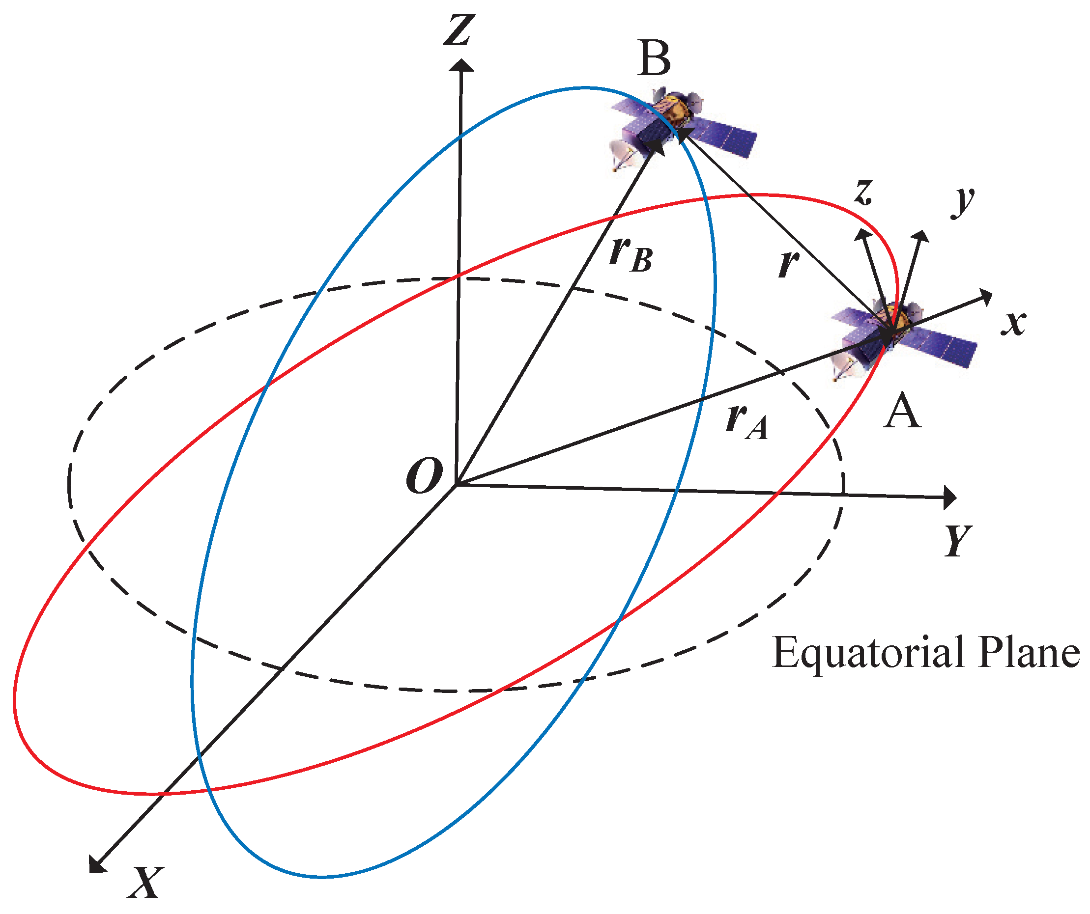
2.1. Coordinate System of Relative Motion

In the study of the relative motion of spacecraft, the following model is established. The main spacecraft is A, the accompanying spacecraft is B, the size of the spacecraft is disregarded, and the earth is regarded as a uniform sphere. The relative motion model of spacecraft A and B in space is shown in Figure 1.

As shown in Figure 1, the geocentric inertial coordinate system is $O–XYZ$, the origin is the geocenter O, the X axis is located in the equatorial plane, the direction points to the vernal point, the Z axis points to the North Star, and the Y axis is determined by the right-hand rule. The relative motion coordinate system of the main spacecraft is $A–xyz$, the origin is A, and the x axis is located over the geocenter, which points to the origin A. The y axis is perpendicular to the x axis and points to the motion direction of the main spacecraft, the z axis is determined by the right-hand rule, the relative positions of spacecraft A and B to the geocenter O are $r_A$ and $r_B$, respectively, and r is the relative position vector of spacecraft A and B.

2.2. Relative Motion Equation

We assume that the reference orbit of the spacecraft is a near-Earth circular orbit without considering any perturbation and that the magnitudes of the relative positions of the spacecraft are much smaller than their distance to the center of Earth. On the one hand, because the spacecraft cluster reconstruction is generally completed within one orbital cycle, the impact of the error dispersion over time due to the nonlinear term in the C-W equation is limited and satisfies the conditions for the application of the C-W equation. On the other hand, the C-W equation with relative position and relative velocity as state variables is simpler than the model based on the orbital elements both in terms of calculating the fuel consumption required for the reconfiguration path and in constructing the avoidance risk of the spacecraft. The relative motion of the spacecraft is described by the following C-W equation [20]:

$$\left\{\begin{array}{c}\ddot{x}-2n\dot{y}-3n^{2}x=u_x\hfill \\ \ddot{y}+2n\dot{x}=u_y\hfill \\ \ddot{z}+n^{2}z=u_z\hfill \end{array}\right.$$

(1)

where n is the angular velocity of the spacecraft and $u_x$, $u_y$, and $u_z$ are the triaxial components of acceleration.

When $t=0$, the state of the spacecraft is ${[x,y,z,\dot{x},\dot{y},\dot{z}]}^T={[x_0,y_0,z_0,{\dot{x}}_0,{\dot{y}}_0,{\dot{z}}_0]}^T$. When $[u_x,u_y,u_z]=[0,0,0]$, the position of the spacecraft in the relative motion coordinate system is expressed as follows:

$$x\left(t\right)=\frac{{\dot{x}}_0}{n}sinnt-(\frac{2{\dot{y}}_0}{n}+3x_0)cosnt+2(\frac{{\dot{y}}_0}{n}+2x_0)$$

(2)

$$y\left(t\right)=2(\frac{2{\dot{y}}_0}{n}+3x_0)sinnt+\frac{2{\dot{x}}_0}{n}cosnt-3({\dot{y}}_0+2n{x}_0)t+(y_0-\frac{2x_0}{n})$$

(3)

$$z\left(t\right)=\frac{{\dot{z}}_0}{n}sinnt+z_{0}cosnt$$

(4)

3. Path Planning Fitness Function Design

In the study of the path planning of spacecraft cluster orbit reconstruction, each maneuver of the spacecraft during orbit transfer changes the instantaneous velocity, which directly affects the fuel consumption. We set the optimal fitness value as meeting the optimum of avoiding threats while consuming the least amount of fuel, and constructed a diagram of the fitness function for path planning, which is shown in Figure 2.

3.1. Performance Index Based on Fuel Consumption

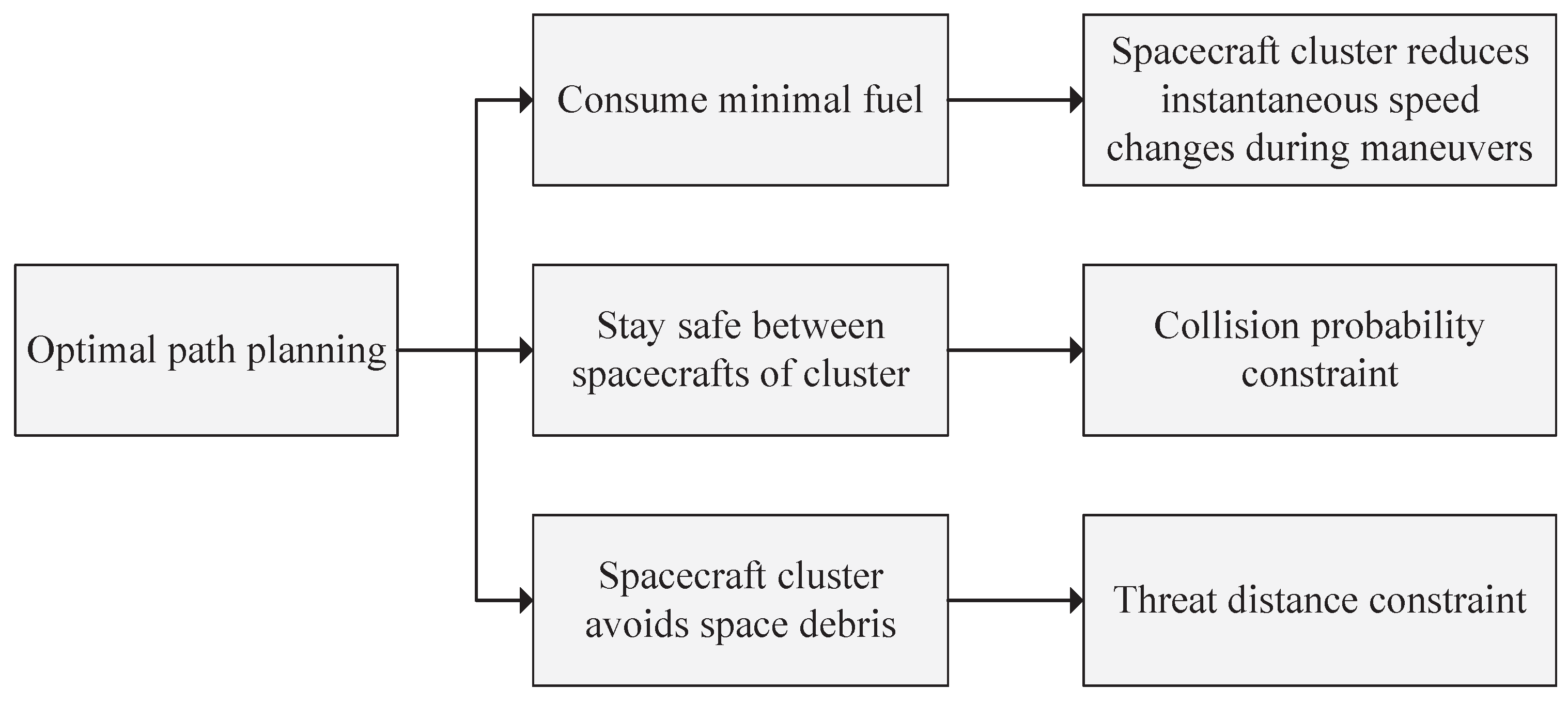
The waypoints are discretized and the fuel consumption during maneuvering is represented by calculating the speed increment $\Delta v\left(i\right)$ at the ith discrete point. The velocities $v{\left(i\right)}^{-}$ and $v{\left(i\right)}^{+}$ before and after the maneuver at the ith discrete point are expressed as follows [21]:

$$\left\{\begin{array}{c}v{\left(i\right)}^{-}={\varphi }_{vr}\left(t\right)P(i-1)+{\varphi }_{vv}\left(t\right)v{(i-1)}^{+}\hfill \\ v{\left(i\right)}^{+}=-{{\varphi }_{rv}}^{-1}\left(t\right){\varphi }_{rr}\left(t\right)P\left(i\right)\hfill \end{array}\right.$$

(5)

where the position of the ith discrete point in the relative motion coordinates is $P\left(i\right)$, and ${\varphi }_{vv}\left(t\right)$, ${\varphi }_{rr}\left(t\right)$, ${\varphi }_{vr}\left(t\right)$, and ${\varphi }_{rv}\left(t\right)$ are the following C-W matrices:

$${\varphi }_{vv}\left(t\right)=\left[\begin{array}{ccc}cosnt& 2sinnt& 0\\ -2sinnt& 4cosnt-3& 0\\ 0& 0& cosnt\end{array}\right]$$

(6)

$${\varphi }_{rr}\left(t\right)=\left[\begin{array}{ccc}4-cosnt& 0& 0\\ 6(sinnt-nt)& 1& 0\\ 0& 0& cos\left(nt\right)\end{array}\right]$$

(7)

$${\varphi }_{vr}\left(t\right)=\left[\begin{array}{ccc}3nsinnt& 0& 0\\ 6n(cosnt-1)& 0& 0\\ 0& 0& -nsinnt\end{array}\right]$$

(8)

$${\varphi }_{rv}\left(t\right)=\left[\begin{array}{ccc}\frac{1}{n}sinnt& \frac{2}{n}(1-cosnt)& 0\\ \frac{2}{n}(cosnt-1)& \frac{1}{n}(4sinnt-3nt)& 0\\ 0& 0& \frac{1}{n}sinnt\end{array}\right]$$

(9)

Because the continuous small thrust provides less thrust, the orbit change time is longer, and the spacecraft cluster can be expected to complete the orbit reconfiguration in a shorter time during the mission. Therefore, this paper considers the use of impulse thrust. Assuming that the number of impulses is d, the speed increment at the ith pulse point is $\Delta v\left(i\right)=v{\left(i\right)}^{+}-v{\left(i\right)}^{-}$. Using the form of the speed increment as a performance index of fuel consumption, the total speed increment in the path is expressed as follows:

$$F_1\left(i\right)=\sum _{i=1}^d∥\Delta v\left(i\right)∥$$

(10)

3.2. Constraints

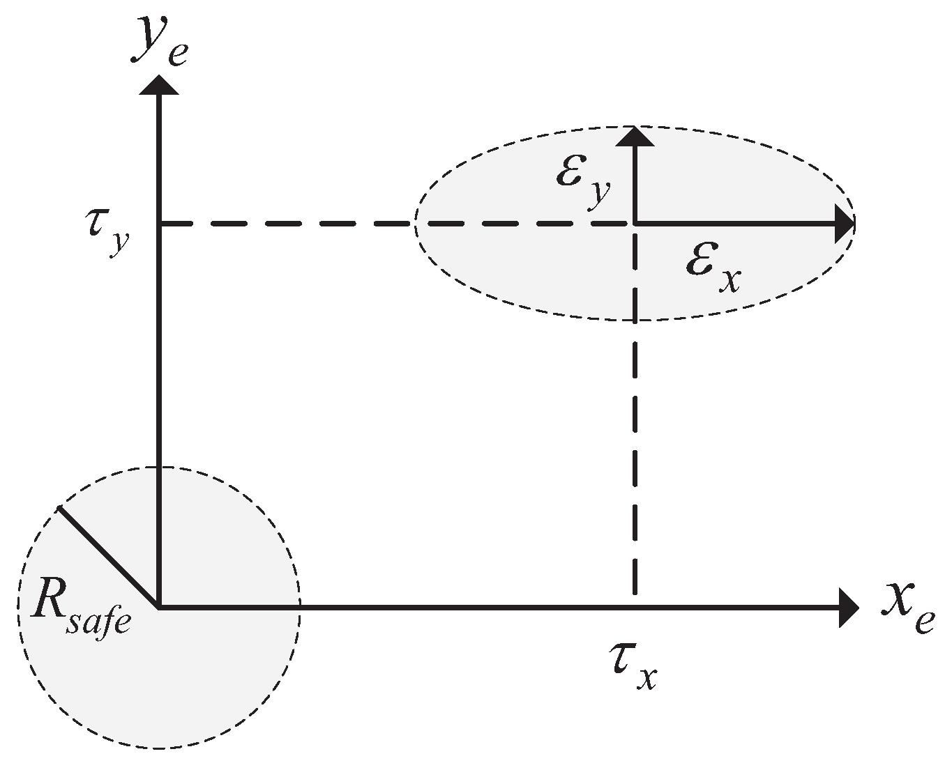
3.2.1. Keeping a Safe Distance between Two Spacecraft Inside the Cluster

To avoid collisions between spacecraft and the interior of the cluster, it is necessary to design the function of safety fitness to establish the minimum safe area. Orbit reconstruction is completed in low orbit, as the spacecraft cluster can accurately calculate the relative position, relative velocity, and relative position covariance matrix of the rendezvous spacecraft during the rendezvous. The collision probability is employed as a constraint to prevent collision within the spacecraft cluster [22]. Selecting the two spacecraft in Figure 1 as an example, when calculating the collision probability, the rendezvous spacecraft A and B are regarded as spheres and the radii are $R_A$ and $R_B$, respectively. Next, the safe radius of the total envelope sphere at the time of the rendezvous is $R_{safe}=R_A+R_B$.

Because the relative position of the spacecraft reaches the minimum during the rendezvous, the relative velocity vector is zero. Therefore, instead of considering the position error due to the direction of the relative velocity, only the collision probability of the spacecraft in the rendezvous plane is considered. As shown in Figure 3, the error ellipse is obtained by projecting the joint error ellipsoid of the intersecting coordinate system onto the rendezvous plane. The origin of the rendezvous plane is defined as the centroid of the enveloping sphere, and the directions of the horizontal axis $x_e$ and vertical axis $y_e$ are parallel to the semimajor axis ${\tau }_x$ of the ellipse and short semiaxis ${\tau }_y$ of the ellipse, respectively. When the distance between the center of mass of the rendezvous sphere and the center of mass of the ellipse is less than $R_{safe}$, this is considered as the two spacecraft colliding. The collision probability P on the rendezvous plane is expressed as follows:

$$P=\frac{1}{2\pi {\epsilon }_x{\epsilon }_y}\underset{S}{\int \int }exp\left\{-\frac{1}{2}\left[\frac{{(x_e-{\tau }_x)}^2}{{{\epsilon }_x}^2}+\frac{{(y_e-{\tau }_y)}^2}{{{\epsilon }_y}^2}\right]\right\}d{x}_{e}d{y}_e$$

(11)

where S is the area of $x_e^2+y_e^2\le R_{safe}$ and ${\epsilon }_x$ and ${\epsilon }_y$ are the standard deviations of the position error on the coordinates of the rendezvous plane.

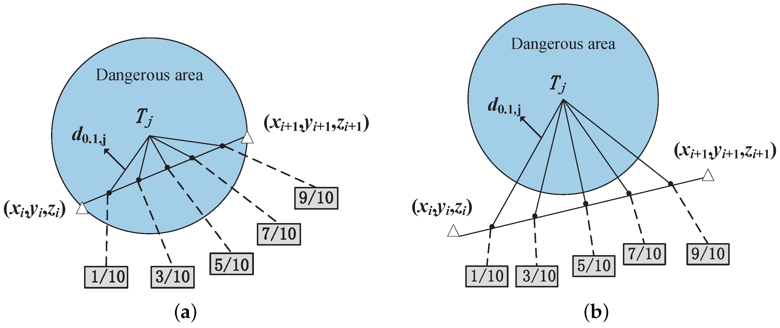
3.2.2. Spacecraft Maintain a Safe Distance Constraint from Other Space Targets

The amount of space debris has dramatically increased in recent decades [23], and spacecraft missions must consider avoiding both other satellites and space debris, which can pose a great threat to the spacecraft orbit transfer process [24]. However, the motion of space debris is extremely irregular [25,26,27], and the relative position, relative velocity, and relative position covariance matrix between space debris and spacecraft cannot be accurately calculated. Using the collision probability in Section 3.2.1 will inevitably cause false alarms [28], resulting in spacecraft performing unnecessary maneuvers in the safe area and consuming additional fuel. In this paper, irregularly shaped space debris are regarded as dangerous areas, and spacecraft can use detection equipment such as lasers or microwave radar to estimate their position. Because the detected dangerous areas have errors, we chose to expand the dangerous area into a sphere appropriately, a strategy that can further ensure the safety of the path. Figure 4 depicts the relationship between the path and the dangerous area; $(x_i,y_i,z_i)$ and $(x_{i+1},y_{i+1},z_{i+1})$ are the locations of the adjacent maneuver points of the spacecraft, and we use five break points to calculate the threat cost of the path between adjacent maneuver points. The advantage of performing segmentation is to simplify the calculation of the threat cost $F_2\left(i\right)$. Strictly speaking, the spacecraft do not maneuver at these five break points. The motion of the spacecraft cluster when no maneuvering occurs satisfies Equations (2)–(4).

The function of the safety fitness to avoid other targets in space is defined as follows:

$$\left\{\begin{array}{c}{F}_2\left(i\right)=m_1{T}_{-in}\left(i\right)+m_2{T}_{-out}\left(i\right)+m_{3}distance\left(i\right)\hfill \\ distance\left(i\right)={\displaystyle \sum _{k=0}^n}{L}_{i,k}\hfill \end{array}\right.$$

(12)

where $m_1+m_2+m_3=1$, $L_{i,k}$ is the length of the jth planning segment of the ith discrete point, $T_{-in}$ represents the dangerous distance from the ith discrete point to the ($i+1$)th discrete point line segment entering the dangerous area, and $T_{-out}$ is the dangerous distance from the ith discrete point line segment that does not enter the dangerous area to the ($i+1$)th discrete point line segment that does not enter the dangerous area. The relevant parameters are expressed as follows:

$$T\_in\left(i\right)=\left\{\begin{array}{cc}\frac{L_{i,j}}{5}{t}_j{\displaystyle \sum _{j=1}^E}(\frac{1}{d_{0.1,j}^4}+\frac{1}{d_{0.3,j}^4}+\frac{1}{d_{0.5,j}^4}+\frac{1}{d_{0.7,j}^4}+\frac{1}{d_{0.9,j}^4}),\hfill & \left|x_i-T_j\right|<R_j\hfill \\ 0,\hfill & \left|x_i-T_j\right|\ge R_j\hfill \end{array}\right.$$

(13)

$$T\_out\left(i\right)=\left\{\begin{array}{cc}{t}_j{\displaystyle \sum _{j=1}^E}(\frac{1}{d_{0.1,j}^4-R_j^4}+\frac{1}{d_{0.3,j}^4-R_j^4}+\frac{1}{d_{0.5,j}^4-R_j^4}+\frac{1}{d_{0.7,j}^4-R_j^4}+\frac{1}{d_{0.9,j}^4-R_j^4}),\hfill & \left|x_i-T_j\right|>R_j\hfill \\ 0,\hfill & \left|x_i-T_j\right|\le R_j\hfill \end{array}\right.$$

(14)

where E represents the number of dangerous areas and $t_j$, $T_j$, and $R_j$ are the threat level, center position, and radius of the jth space debris, respectively.

The path planning expects the fuel consumption function $F_1\left(i\right)$ to be minimal, and in order for the spacecraft to avoid the threat constraint the collision probability P must be less than the safety threshold and the threat distance $F_2\left(i\right)$ must be greater than the radius of the dangerous area. The interior-point penalty function is employed to solve the objective optimization with constraints [30]. The function of the fitness of path planning is expressed as follows:

$$F\left(i\right)=F_1\left(i\right)+J\{[min(0,log\frac{P_{max}}{max\left(P_n\left(i\right)\right)}){]}^2+[min(0,log\frac{min\left(F_2\left(i\right)\right)}{R_j}){]}^2\}$$

(15)

where J is the penalty coefficient, $P_{max}$ is the threshold of collision probability, and max $\left(Pn\right(i\left)\right)$ represents the maximum probability of collision between adjacent spacecraft.

4. ALPIO for Path Planning

4.1. ALPIO Algorithm Structure

We propose using the ALPIO algorithm to solve the optimal spacecraft cluster orbit reconstruction path planning designed in Section 3. Section 4 mainly introduces ALPIO, which is an improvement on the shortcomings of the traditional PIO. The block diagram of ALPIO is shown in Figure 5.

4.2. Initialization Based on Tent Map Chaotic and Elite Backward Learning

Compared with random numbers, tent map chaos has better coverage and diversity and allows the positions of the pigeons to be uniformly distributed around the optimum [31]. The mathematical formula model is expressed as follows:

$$Y_{i+1}=a(1-2\left|Y_i-0.5\right|),i=0,1,2,\dots$$

(16)

where a is the mapping parameter of the tent map, $a\in (0,4)$. $Y_i$ is the mapping of the tent map, and $0<Y_i<1$.

To further increase the diversity of the population, we selected the elite backward learning strategy to update the position of the initial chaotic population [32] to bring the initial population closer to the global optimum. The position of the ith chaotic initial individual in D-dimensional space is defined as $X_{i,j}=[X_{i,1},X_{i,2}\dots ,X_{i,D}]$, and elite backward learning is defined as follows:

$${\overline{X}}_{i,j}=rand(X_{i,jmin}+X_{i,jmax})-X_{i,jmin}$$

(17)

where $rand$ is a random number between 0 and 1 and $X_{i,jmin}$ and $X_{i,jmax}$ represent the minimum value and maximum value, respectively, of the boundary of the solution.

When Equation (17) is outside the boundary of the solution, the elite backward solution is reset as follows:

$$X_{i,j}^{*}=rand(X_{i,jmin}+X_{i,jmax})$$

(18)

Here, the fitness values corresponding to individuals $X_{i,j}$ and $X_{i,j}^{*}$ are defined as $F\left(i\right)$ and $F^{*}\left(i\right)$, respectively. Consider that when $F^{*}\left(i\right)<F\left(i\right)$, the individual position $X_{i,j}^{*}$ replaces $X_{i,j}$, while otherwise the individual position takes $X_{i,j}$.

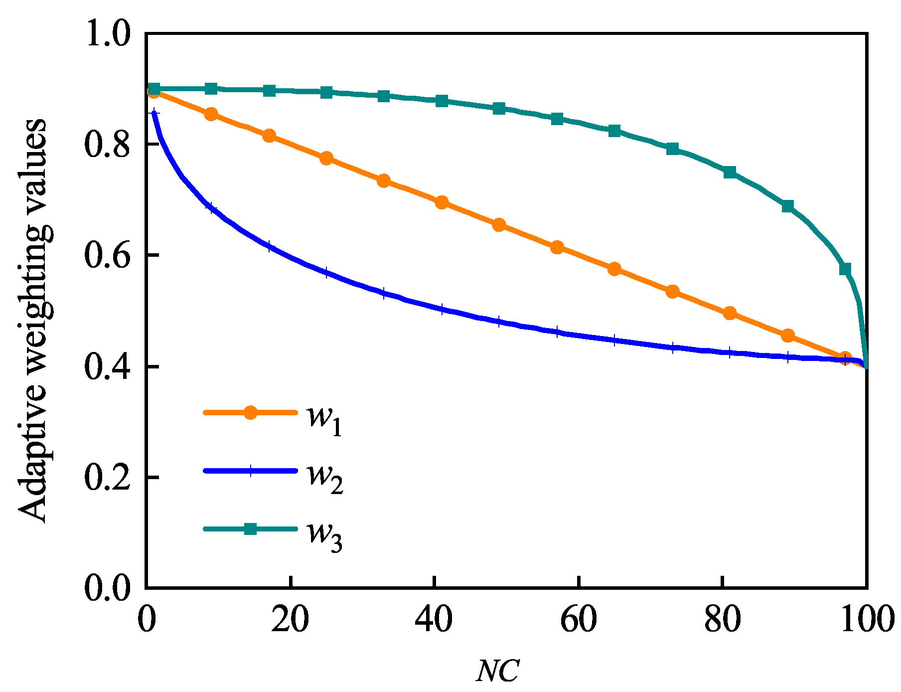
4.3. Nonlinear Adaptive Strategy to Improve Convergence Accuracy

The first stage of the PIO is the map and compass operator, and the mathematical model of the speed and position of the ith pigeon in D-dimensional space are expressed as follows:

$$V_{i,j}^{NC}=V_{i,j}^{NC-1}\times {\mathrm{e}}^{-R\times NC}+rand(X_g-X_{i,j}^{NC-1})$$

(19)

$$X_{i,j}^{NC}=X_{i,j}^{NC-1}+V_{i,j}^{NC}$$

(20)

where R is the compass factor, $NC$ is the number of current iterations, and $X_g$ represents the local optimal solution.

The first stage is a rough search process, and the individual with the best fitness value is determined by comparing the positions of the pigeons. After the operator completes the iteration, it enters the Landmark Operator; $V_{i,j}^{NC-1}\times {\mathrm{e}}^{-R\times NC}$ represents the speed and direction of the pigeon, which affects the subsequent process of obtaining the optimum for the population. Because the compass factor R is a constant value, when $R=0.6$, $NC=10$, ${\mathrm{e}}^{-R\times NC}\approx 0$, and the algorithm stops the global search, it is easy to fall into a local optimum. When $R=0.03$, the convergence speed is very slow, which reduces the search ability of the population in the early stage. To balance the relationship between the population convergence speed and the global search ability, we introduce a nonlinear adaptive weight factor w instead of ${\mathrm{e}}^{-R\times NC}$. The inertial weight linear decreasing method proposed by Shi is widely utilized to solve the algorithm’s convergence [33]; its formulation is expressed as follows:

$$w_1^{NC}=w_{max}-(w_{max}-w_{min})\frac{NC}{T_1}$$

(21)

where $T_1$ represents the number of iterations of the map and compass operator.

With the aim of establishing a dynamic optimization process of pigeon flocks to avoid falling into local optima, this paper proposes the following two nonlinear decreasing weight factors:

$$\left\{\begin{array}{c}{w}_2^{NC}=w_{max}exp((lnk)/(ln\frac{w_{min}}{NC}\frac{w_{max}}{T_1}))\hfill \\ w_3^{NC}=(w_{max}-w_{min}){(1-{(\frac{NC}{T_1})}^{\gamma })}^{\frac{1}{\gamma }}+w_{min}\hfill \end{array}\right.$$

(22)

Assuming that the number of iterations is 100, the dynamic changes of the three adaptive weight factors are shown in Figure 6.

Figure 6 shows that the value of $w_3$ is large in the early stage and slowly changes, which is beneficial to the global search of the population. Furthermore, the fast convergence of the option value in the later period is conducive to the algorithm jumping out of the local search, which ensures the global optimization ability of the algorithm. For these reasons, $w_3$ is chosen as the nonlinear adaptive weight factor.

While weighting the early convergence speed and global search ability, we introduce the sine adjustment factor C to control the influence of the local optimal solution on the population position in the next iteration.

$$C=sin(\frac{NC}{T_1}·\frac{\pi }{2})$$

(23)

After introducing the nonlinear adaptive weight factor w and adjustment factor C, Equation (19) is updated as Equation (24):

$$V_{i,j}^{NC}=V_{i,j}^{NC-1}(\alpha +\beta w)+(\alpha +\beta C)·rand·(X_{\mathrm{g}}-X_{i,j}^{NC-1})$$

(24)

where $\alpha +\beta =1$.

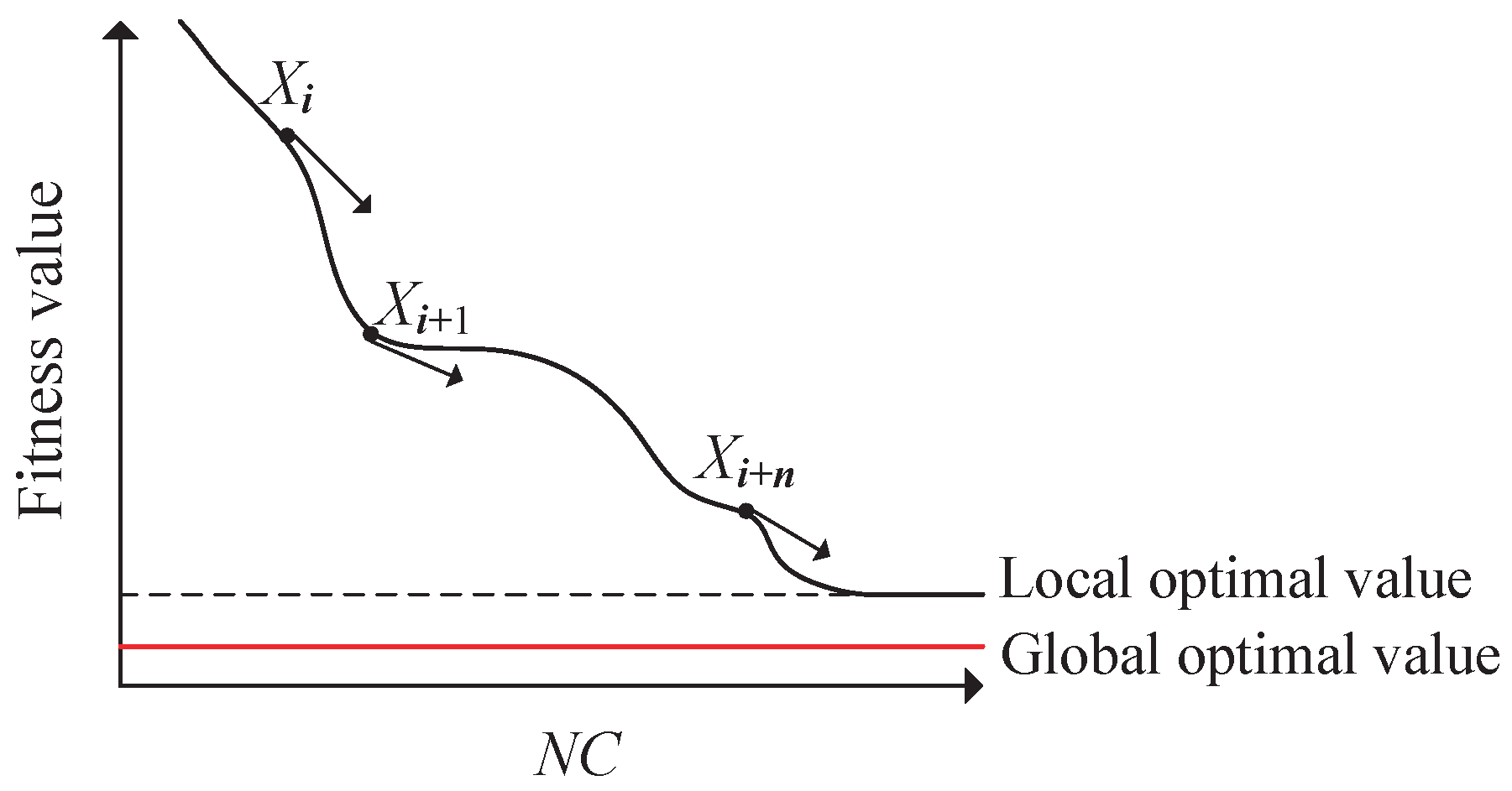
4.4. Cauchy Mutation Strategy for Avoiding Local Optima

The purpose of the rough search in the first stage is to guide the pigeons to quickly identify the optimal position without arriving at the optimal position directly.

As shown in Figure 7, the current individual position $X_i$ is the first to approach the local optimal value in the process of identifying the optimum, while the population is gathered near the local optimal value. Applying mutation to the current position cannot directly reach the global value beyond the local optimal value. Because a characteristic of the Cauchy mutation function is that the extreme value at the origin is small and the distribution at both ends is relatively long, the implementation of Cauchy mutation for the local optimal value can cause the population to jump out of the local optimum. The function of the Cauchy mutation is defined as follows:

$$f\left(x\right)=\frac{1}{\pi }\times \frac{m}{m^2+x^2},x\in (-\infty ,+\infty )$$

(25)

To solve the situation in which the optimization parameters jump outside of the boundary value, we introduce a percentage to describe m in the Cauchy mutation [34]:

$${\int }_{x_{min}}^{x_{max}}\frac{1}{\pi }\frac{m}{m^2+x^2}dx=\frac{1}{\pi }arctan\frac{x}{m}\left|{}_{x_{min}}^{x_{max}}\right.=percent$$

(26)

$$m=\frac{x_{max}-x_{min}}{2tan\frac{percent\times \pi }{2}}$$

(27)

After introducing the Cauchy mutation in Equation (24), it can be updated as Equation (28):

$$V_{i,j}^{NC}=V_{i,j}^{NC-1}(\alpha +\beta w)+(\alpha +\beta C)f_1(X_g+m\times tan\left[\pi (f_2-0.5)\right]-X_{i,j}^{NC-1})$$

(28)

where $f_1$ and $f_2$ are random numbers between 0 and 1. A new dynamic selection strategy is proposed to further improve the performance of the algorithm for determining the optimum. When the population stagnates for a long time, the fitness value updates for twenty consecutive iterations and does not exceed 0.01, indicating that the population is likely to fall into a local optimum. Next, the Cauchy mutation is imposed, that is, Equation (28) is applied as the first stage of optimization; otherwise, Equation (24) is applied. The advantage of this dynamic selection strategy is that it can accelerate the convergence rate when it does not fall into the local optimum in the early stage.

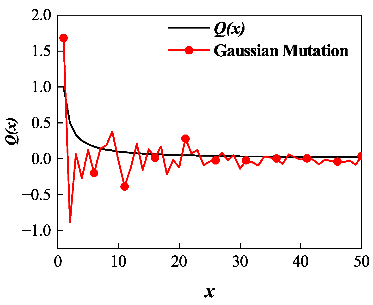
4.5. Gaussian Mutation Strategy to Prevent Population Evolution from Stagnation

The second stage of the PIO is the landmark operator [11]. The number of pigeons in each iteration is halved, and the center position of the remaining pigeons is used as a reference. The mathematical model of the landmark operator is expressed as follows:

$$M_p^{NC}=\frac{M_p^{NC-1}}{2}$$

(29)

$$X_c^{NC}=\frac{\sum X_{i,j}^{NC}\times F\left(X_{i,j}^{NC}\right)}{M_p^{NC}\times \sum F\left(X_{i,j}^{NC}\right)}$$

(30)

$$X_{i,j}^{NC}=X_{i,j}^{NC-1}+rand\times (X_c^{NC-1}-X_{i,j}^{NC-1})$$

(31)

where $M_p^{NC}$, $X_c^{NC}$, and $F\left(X_{i,j}^{NC}\right)$ are the number of individuals in the $NC$th iteration, the center position of the remaining population, and the fitness function of the individual, respectively.

Because the pigeons entering the landmark operator are already near the global optimal value, a fine search is needed, and the global optimal value can be reached without too much mutation. Here, we employ Gaussian mutation at the center of the population to solve the problem of late population evolution stagnation; the function of the Gaussian mutation [35] is expressed as follows:

$$N\left(x\right)=\frac{1}{\sigma \times \sqrt{2\pi }}\times exp(-\frac{{(x-\mu )}^2}{2{\sigma }^2})$$

(32)

where $\mu$ and ${\sigma }^2$ are the mean and variance, respectively.

By setting the function $Q\left(x\right)=x^{-1},x\in [1,50]$, as shown in Figure 8, it can be seen that the value after adding Gaussian mutation to $Q\left(x\right)$ slightly fluctuates around the original value.

In the landmark operator, if the number of pigeons decreases too fast it can affect the search. We therefore add the hyperbolic sine variation factor B to enhance the global search ability of the pigeon. The formulation of the hyperbolic sine variation factor B is expressed as follows:

$$B=1-\frac{T_2}{5}\times sinh\frac{N{C}^3}{100\times T_2^3}$$

(33)

where $T_2$ is the number of iterations of the landmark operator.

After introducing the variation factor B and Gaussian mutation, the mathematical model of the population position in Equation (31) is updated as follows:

$$X_{i,j}^{NC}=X_{i,j}^{NC-1}+B\times (X_c^{NC-1}\times (1+G_s(\mu ,{\sigma }^2)-X_{i,j}^{NC-1}))$$

(34)

where $G_s(\mu ,{\sigma }^2)$ is the Gaussian mutation.

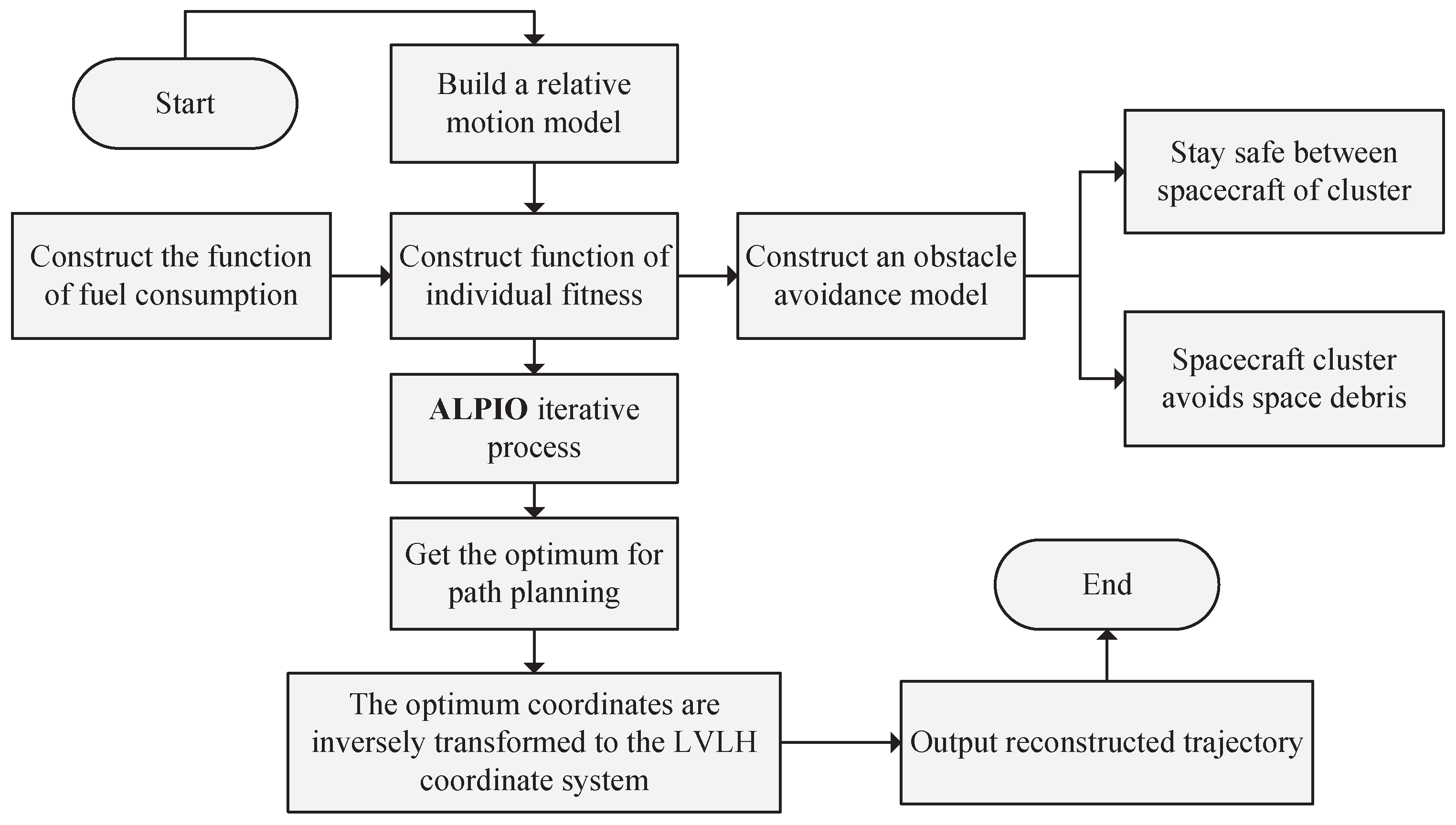
4.6. Scheme of Path Planning of Orbit Reconstruction

In order to simplify the complexity of path planning, this paper takes the initial position of each spacecraft in the LVLH coordinate system and the line where the target position is located as the new $x_r$ axis, considers that the direction is from the initial position to the target position, and uses the trajectory obtained via ALPIO to construct a new $y_r$ axis and $z_r$ axis to describe the orbit reconstruction trajectory. The ALPIO algorithm realizes the path planning process of spacecraft cluster orbit reconstruction, as shown in Figure 9.

5. Simulation Experiment and Result Analysis

5.1. Track Reconstruction Path Planning

In order to verify the convergence ability and stability of ALPIO, the minimum values of nine benchmark functions, including single-peak and multipeak functions, were tested in comparison with PSO, PIO, and CGAPIO [35]. The number of populations for all four algorithms was 30, the dimensionality was 20, the number of iterations for PSO was 100, and the other algorithm parameters were as shown in

Table 1. Parameters for initialization of the algorithm.

Parameter	Expression	Value
a	Mapping parameter of Tent Map	1
$X_0$	Initial value of Tent Map	0.32
$w_{\min }$	Minimum value of weighting factor	0.40
$w_{\max }$	Maximum value of weighting factor	0.90
$\gamma$	Parameters of weighting factor	2.50
R	Compass factor	0.30
$T_1$	Number of iterations of Map and Compass Operator	60
$T_2$	Number of iterations of the Landmark Operator	40

. The test functions are shown in

Table 2. Test functions.

Functions	Expression	Range	Min
Sphere	$f_1\left(x\right)={\sum }_{i=1}^D{x}_i^2$	$[-100,100]$	0
Schwefel_2.21	$f_2\left(x\right)=max\left\{\left|x_i\right|\right\}$	$[-100,100]$	0
Schwefel_2.22	$f_3\left(x\right)={\sum }_{i=1}^D\left|x_i\right|+{\prod }_{i+1}^D\left|x_i\right|$	$[-10,10]$	0
Setp	$f_4\left(x\right)={\sum }_{i=1}^D{\left|x_i+0.5\right|}^2$	$[-100,100]$	0
Rastrigin	$f_5\left(x\right)=10D+{\sum }_{i=1}^D(x_i^2-10cos\left(2\pi x_i\right))$	$[-5,5]$	0
Ackley	$f_6\left(x\right)=20-20exp(-0.2\sqrt{\frac{1}{D}{\sum }_{i=1}^D{x}_i^2})-exp\left(\frac{1}{D}{\sum }_{i=1}^{D}cos\left(2\pi x_i\right)\right)+\mathrm{e}$	$[-40,40]$	0
Griewank	$f_7\left(x\right)=\frac{1}{4000}{\sum }_{i=1}^D{x}_i^2-{\prod }_{i+1}^{D}cos\left(\frac{x_i}{\sqrt{i}}\right)+1$	$[-600,600]$	0
Rosenbrock	$f_8\left(x\right)={\sum }_{i=1}^{D-1}[100(x_{i+1}-x_i^2)+{(x_i-1)}^2]$	$[-30,30]$	0
Apline	$f_9\left(x\right)={\sum }_{i=1}^D\left|x_{i}sin\left(x_i\right)+0.1x_i\right|$	$[-10,10]$	0

.

The results of the function tests are shown in

Table 3. Results of the function test.

Functions	Algorithm	Min	STD
Sphere	PSO PIO CGAPIO ALPIO	2.22 $\times {10}^{-5}$ 1.21 $\times {10}^{-2}$ 6.17 $\times {10}^{-6}$ 8.94 $\times {10}^{-9}$	3.27 $\times {10}^0$ 2.65 $\times {10}^1$ 2.83 $\times {10}^{-2}$ 1.22 $\times {10}^{-5}$
Schwefel_2.21	PSO PIO CGAPIO ALPIO	9.16 $\times {10}^{-3}$ 6.22 $\times {10}^{-4}$ 5.60 $\times {10}^{-4}$ 6.58 $\times {10}^{-6}$	2.18 $\times {10}^0$ 3.58 $\times {10}^0$ 5.82 $\times {10}^{-1}$ 6.19 $\times {10}^{-3}$
Schwefel_2.22	PSO PIO CGAPIO ALPIO	5.99 $\times {10}^{-2}$ 2.65 $\times {10}^0$ 2.45 $\times {10}^{-3}$ 1.28 $\times {10}^{-5}$	7.32 $\times {10}^{-1}$ 3.82 $\times {10}^0$ 2.54 $\times {10}^{-2}$ 7.21 $\times {10}^{-4}$
Setp	PSO PIO CGAPIO ALPIO	4.75 $\times {10}^{-11}$ 9.89 $\times {10}^{-7}$ 2.87 $\times {10}^{-3}$ 2.95 $\times {10}^{-10}$	3.68 $\times {10}^0$ 5.49 $\times {10}^1$ 3.27 $\times {10}^1$ 2.87 $\times {10}^{-1}$
Rastrigin	PSO PIO CGAPIO ALPIO	1.00 $\times {10}^1$ 2.12 $\times {10}^{-2}$ 9.95 $\times {10}^{-1}$ 3.49 $\times {10}^{-5}$	6.94 $\times {10}^0$ 2.45 $\times {10}^1$ 1.95 $\times {10}^{-2}$ 8.45 $\times {10}^{-3}$
Ackley	PSO PIO CGAPIO ALPIO	1.68 $\times {10}^1$ 1.77 $\times {10}^1$ 4.37 $\times {10}^{-5}$ 5.01 $\times {10}^{-8}$	3.31 $\times {10}^0$ 1.29 $\times {10}^0$ 5.58 $\times {10}^{-1}$ 6.86 $\times {10}^{-3}$
Griewank	PSO PIO CGAPIO ALPIO	7.34 $\times {10}^1$ 1.19 $\times {10}^0$ 1.51 $\times {10}^0$ 5.31 $\times {10}^{-3}$	1.97 $\times {10}^{-1}$ 6.57 $\times {10}^{-1}$ 1.36 $\times {10}^{-1}$ 2.81 $\times {10}^{-2}$
Rosenbrock	PSO PIO CGAPIO ALPIO	1.18 $\times {10}^2$ 2.83 $\times {10}^1$ 1.90 $\times {10}^1$ 1.00 $\times {10}^1$	1.84 $\times {10}^2$ 2.65 $\times {10}^3$ 1.02 $\times {10}^{-1}$ 1.32 $\times {10}^{-3}$
Apline	PSO PIO CGAPIO ALPIO	3.96 $\times {10}^1$ 4.13 $\times {10}^{-2}$ 5.98 $\times {10}^{-6}$ 4.25 $\times {10}^{-8}$	5.25 $\times {10}^1$ 1.47 $\times {10}^1$ 4.89 $\times {10}^{-2}$ 3.67 $\times {10}^{-3}$

, and the data in Table 3 correspond to the convergence curves in Figure 10. The standard deviation of ALPIO is the smallest among the nine experiments, which indicates that ALPIO is more stable than other optimization methods. By comparing the convergence minimum of the tested function with the theoretical minimum, these results show the higher accuracy of convergence with ALPIO.

5.2. Simulation of Different Algorithms for Path Planning

In this paper, we do not consider the effect of any perturbation on the orbit in path planning. Based on the conditions when using the C-W equation, only the relative states of the spacecraft, the obstacle, and the reference spacecraft are considered, and any change in position between the obstacles and the reference spacecraft is ignored in the LVLH coordinate system. The reference spacecraft is set as the coordinate origin in LVLH; its semi-major axis is 7178.14 km, with eccentricity ${10}^{-6}$, inclination ${98}^{\circ }$, right ascension of ascending node $194.{224}^{\circ }$, argument of perigee $0^{\circ }$, and true anomaly $0^{\circ }$. To verify that the proposed ALPIO-based approach avoids the obstacle environment, consumes the least fuel, and improves the smoothness of the path when applying spacecraft cluster orbit reconstruction path planning, the fuel consumption, fitness value of the algorithms, and smoothness of the trajectory of each spacecraft were compared with the basic PSO, basic PIO, and CGAPIO. The parameters of the simulation were set as shown in

Table 4. Initial relative state parameters of the spacecraft and obstacles.

	x/(km)	y/(km)	z/(km)	$\dot{\mathit{x}}$/(km/s)	$\dot{\mathit{y}}$/(km/s)	$\dot{\mathit{z}}$/(km/s)
Spacecratf1	0	40	2	−0.002	0	$-2.4\times {10}^{-4}$
Spacecraft2	−40	0	1.2	0.002	0.002	$-2\times {10}^{-4}$
Spacecratf3	0	−40	2	−0.002	0	$-1.6\times {10}^{-4}$
Spacecratf4	40	0	2.8	0	−0.002	$-2\times {10}^{-4}$
Obstacle1	0	27	0	−0.002	0	$-2.4\times {10}^{-4}$
Obstacle2	−26	0	0	0.002	0.002	$-2\times {10}^{-4}$
Obstacle3	0	−28	0	−0.002	0	$-1.6\times {10}^{-4}$
Obstacle4	25	0	0	0	−0.002	$-2\times {10}^{-4}$

,

Table 5. Target relative state parameters of spacecraft.

	x/(km)	y/(km)	z/(km)	$\dot{\mathit{x}}$/(km/s)	$\dot{\mathit{y}}$/(km/s)	$\dot{\mathit{z}}$/(km/s)
Spacecratf1	14.14	−14.14	−1.71	0	0	0
Spacecraft2	14.14	14.14	−1.71	0	0	0
Spacecratf3	−14.14	14.14	−2.28	0	0	0
Spacecratf4	−14.14	−14.14	−2.28	0	0	0

and

Table 6. Parameters of path planning.

Parameter	Expression	Value
J	Penalty factor	100
$P_{max}$	Threshold of collision probability	${10}^{-6}$
n	Orbital angular velocity	${10}^{-3}$ rad/s
t	Reconstruction time	≤40 min
$R_{safe}$	Safe distance	30 m
$u_x,u_y,u_z$	Acceleration components	${10}^{-5}$ m/s ${}^2$

. The data in Table 4 and Table 5 indicate the relative states with the reference satellite, while the initialization parameters of the algorithms are shown in Table 1.

The results of the simulation are shown in Figure 11. The blue orbit and red orbit are the initial transfer orbit and target transfer orbit, respectively, of the spacecraft, and the colored spheres represent obstacles in space.

5.3. Comparison of Fuel Consumption with Different Algorithms

As shown in

Table 7. Four-Impulse.

Algorithm	$\Delta \mathit{v}$/(km/s)
	Spacecraft 1	Spacecraft 2	Spacecraft 3	Spacecraft 4	Total
PSO	0.143930	0.179476	0.151393	0.197614	0.672413
PIO	0.141176	0.175323	0.141251	0.177637	0.635388
CGAPIO	0.140877	0.173518	0.140907	0.175290	0.630592
ALPIO	0.140823	0.173353	0.140866	0.175288	0.630333

,

Table 8. Five-Impulse.

Algorithm	$\Delta \mathit{v}$/(km/s)
	Spacecraft 1	Spacecraft 2	Spacecraft 3	Spacecraft 4	Total
PSO	0.154627	0.210988	0.162819	0.200227	0.728661
PIO	0.157961	0.193940	0.156199	0.192466	0.700566
CGAPIO	0.150595	0.182973	0.157982	0.198670	0.690220
ALPIO	0.146349	0.176344	0.144906	0.194798	0.662397

and

Table 9. Six-Impulse.

Algorithm	$\Delta \mathit{v}$/(km/s)
	Spacecraft 1	Spacecraft 2	Spacecraft 3	Spacecraft 4	Total
PSO	0.193661	0.271571	0.179255	0.212045	0.856532
PIO	0.163336	0.197146	0.163789	0.200310	0.724581
CGAPIO	0.163417	0.192411	0.157560	0.202538	0.715926
ALPIO	0.156120	0.183607	0.149306	0.200546	0.689579

, the total consumption of fuel for orbital reconstruction increases for each algorithm under the same conditions as the number of impulses. Compared with the other algorithms, ALPIO maintains the least consumption of fuel for different impulses. The problem becomes more complicated regarding the search for a better trajectory solution due to the increase in the number of trajectory discretization points. Therefore, we consider the use of four impulses to complete the trajectory reconstruction of the cluster. The time required by different algorithms to complete path planning with different numbers of impulses is shown in

Table 10. Running time of different algorithms at different impulses.

Algorithm	Running Time/(s)
	Four-Impulse	Five-Impulse	Six-Impulse
PSO	7.76	9.89	12.39
PIO	5.48	6.73	10.28
CGAPIO	5.29	6.55	9.96
ALPIO	5.12	6.34	9.52

. The results indicate that the real-time performance of the ALPIO proposed in this paper represents a great improvement.

5.4. Comparison of Fitness Value Changes of Different Algorithms

Figure 12 shows the fitness value curve of each algorithm with different impulses. It can be clearly seen that the PSO falls into the local optimum in the early stage. Compared with PIO, ALPIO jumps out of the local optimum in the later stage while maintaining fast convergence. The convergence speed of ALPIO is faster than that of CGAPIO, and the convergence accuracy is improved, as well which again proves that ALPIO has better convergence.

5.5. Comparison of the Smoothness of the Path Planning Trajectory with Different Algorithms

Selecting Spacecraft 2 and 4 in Figure 11 as the reference spacecraft, the starting points and target points are transformed to the $x_r$ axis in the new coordinate system in Section 4.6. The $y_r$ axis and $z_r$ axis are used as the reference directions. The components of the reconstructed trajectory points planned by different algorithms on the $y_r$ axis and $z_r$ axis are compared with the distance variation range from the reference direction, with a smaller change indicating a smoother trajectory.

Figure 13, Figure 14, Figure 15 and Figure 16 show the comparison of the trajectories of the four spacecraft using different algorithms to complete the path planning, respectively. Each path is compared with the reference axis. Note that the red line is smoother than the other three lines, indicating that the smoothness of the trajectory in the path planned by ALPIO is improved; this can reduce the jitter of the spacecraft during maneuvers, further ensuring its safety.

5.6. Comparison of Obstacle Avoidance

In spacecraft cluster orbit reconstruction, the threat distances of all paths of the spacecraft cluster are considered. Figure 17 represents the sum of the threat distances at each moment; in combination with Figure 11, it can be seen that each path does not enter the dangerous areas. Thus, the threat distance consists of the distance between the paths outside the region and the discrete points. It is obvious that a farther distance between the discrete points and the center of the danger means a larger $F_2$, i.e., the threat distance at the maneuver point increases, According to Figure 17, the threat distance corresponding to PSO is unstable; the value is larger than other algorithms, indicating that the safe path further bypasses the dangerous area. The threat distance corresponding to ALPIO fluctuates less than the other algorithms, and the value is smaller, indicating that the spacecraft is in the safe area and the path does not bypass the dangerous area by very much, which can save fuel while meeting the requirements of optimal path planning.

6. Conclusions

The proposed ALPIO-based approach can solve the inherent problems of PIO, that is, is able to escape both local optima and late evolutionary stagnation. Different mutation strategies are applied for the optimal search characteristics of pigeons at different stages, while the number of pigeons is always kept at a reasonable size during the evolution of the population, balancing the speed of convergence and the local search capability.

The convergence accuracy of ALPIO is better at reaching the optimal solution, and the algorithm is able to solve the obstacle avoidance problem between spacecraft and space targets in the path planning of spacecraft cluster orbit reconstruction. Compared with the path planned by PIO, the degree of smoothness is greatly improved, which can further ensure the safety of the spacecraft in path planning.

References

1. Hanson, J.; Chartres, J.; Sanchez, H.; Oyadomari, K. The EDSN intersatellite communications architecture. In Proceedings of the Annual AIAA/USU Conference on Small Satellites, Logan, UT, USA, 14–17 August 2014. [Google Scholar]
2. Clark, P.; Rilee, M.; Curtis, S.; Truszkowski, W.; Marr, G.; Cheung, C.; Rudisill, M. BEES for ANTS: Space mission applications for the autonomous nanotechnology swarm. In Proceedings of the AIAA 1st Intelligent Systems Technical Conference, Chicago, IL, USA, 20–22 September 2004; p. 6303. [Google Scholar]
3. Akioka, M.; Nagatsuma, T.; Miyake, W.; Ohtaka, K.; Marubashi, K. The L5 mission for space weather forecasting. Adv. Space Res. 2005, 35, 65–69. [Google Scholar] [CrossRef]
4. Němec, F.; Kotková, M. Evaluating the Accuracy of Magnetospheric Magnetic Field Models Using Cluster Spacecraft Magnetic Field Measurements. Universe 2021, 7, 282. [Google Scholar] [CrossRef]
5. Chu, J.; Guo, J.; Gill, E. A survey of autonomous cooperation of modules’ cluster operations for fractionated spacecraft. Int. J. Space Sci. Eng. 2013, 1, 3–19. [Google Scholar] [CrossRef]
6. Xu, M.; Liang, Y.; Tan, T.; Wei, L. Cluster flight control for fractionated spacecraft on an elliptic orbit. Celest. Mech. Dyn. Astron. 2016, 125, 383–412. [Google Scholar] [CrossRef]
7. Wang, W.; Wu, D.; Lei, H.; Baoyin, H. Fuel-Optimal Spacecraft Cluster Flight Around an Ellipsoidal Asteroid. J. Guid. Control Dyn. 2021, 44, 1875–1882. [Google Scholar] [CrossRef]
8. Fowler, K.; Teixeira-Dias, F. Hybrid Shielding for Hypervelocity Impact of Orbital Debris on Unmanned Spacecraft. Appl. Sci. 2022, 12, 7071. [Google Scholar] [CrossRef]
9. Zhu, Z.; Qian, Y.; Zhang, W. Research on UAV Searching Path Planning Based on Improved Ant Colony Optimization Algorithm. In Proceedings of the 2021 IEEE 3rd International Conference on Civil Aviation Safety and Information Technology (ICCASIT), Changsha, China, 20–22 October 2021; pp. 1319–1323. [Google Scholar]
10. Rokbani, N.; Neji, B.; Slim, M.; Mirjalili, S.; Ghandour, R. A Multi-Objective Modified PSO for Inverse Kinematics of a 5-DOF Robotic Arm. Appl. Sci. 2022, 12, 7091. [Google Scholar] [CrossRef]
11. Duan, H.; Qiao, P. Pigeon-inspired optimization: A new swarm intelligence optimizer for air robot path planning. Int. J. Intell. Comput. Cybern. 2014, 7, 24–37. [Google Scholar] [CrossRef]
12. Yuan, G.; Xia, J.; Duan, H. A continuous modeling method via improved pigeon-inspired optimization for wake vortices in UAVs close formation flight. Aerosp. Sci. Technol. 2022, 120, 107259. [Google Scholar] [CrossRef]
13. Hua, B.; Huang, Y.; Wu, Y.; Chen, Z.; Nicholas, D. Spacecraft formation reconfiguration trajectory planning with avoidance constraints using adaptive pigeon-inspired optimization. Sci. China Inf. Sci. 2019, 62, 70209. [Google Scholar] [CrossRef]
14. Xian, N.; Chen, Z. A quantum-behaved pigeon-inspired optimization approach to explicit nonlinear model predictive controller for quadrotor. Int. J. Intell. Comput. Cybern. 2018, 11, 47–63. [Google Scholar] [CrossRef]
15. Pei, J.; Su, Y.; Zhang, D. Fuzzy energy management strategy for parallel HEV based on pigeon-inspired optimization algorithm. Sci. China Technol. Sci. 2017, 60, 425–433. [Google Scholar] [CrossRef]
16. Lyu, Y.; Zhang, Y.; Chen, H. An Improved Pigeon-Inspired Optimization for Multi-focus Noisy Image Fusion. J. Bionic Eng. 2021, 18, 1452–1462. [Google Scholar] [CrossRef]
17. Yuan, Y.; Duan, H. Active disturbance rejection attitude control of unmanned quadrotor via paired coevolution pigeon-inspired optimization. Aircr. Eng. Aerosp. Technol. 2021, 94, 302–314. [Google Scholar] [CrossRef]
18. Mirjalili, S. Evolutionary algorithms and neural networks. In Studies in Computational Intelligence; Springer: Berlin/Heidelberg, Germany, 2019; Volume 780. [Google Scholar]
19. Wang, J.; Song, X.; Le, Y.; Wu, W.; Zhou, B.; Ning, X. Design of self-shielded uniform magnetic field coil via modified pigeon-inspired optimization in miniature atomic sensors. IEEE Sens. J. 2020, 21, 315–324. [Google Scholar] [CrossRef]
20. Ogundele, A.D. Modeling and analysis of nonlinear spacecraft relative motion via harmonic balance and Lyapunov function. Aerosp. Sci. Technol. 2020, 99, 105761. [Google Scholar] [CrossRef]
21. Zhang, S.; Duan, H. Gaussian pigeon-inspired optimization approach to orbital spacecraft formation reconfiguration. Chin. J. Aeronaut. 2015, 28, 200–205. [Google Scholar] [CrossRef]
22. Yang, W.W.; Zhao, Y.; Chen, X.Q.; Wang, Z.G. Progress in calculation methods for collision probability of spacecraft. Chin. Space Sci. Technol. 2012, 32, 8–15. [Google Scholar] [CrossRef]
23. Dolado-Perez, J.; Pardini, C.; Anselmo, L. Review of uncertainty sources affecting the long-term predictions of space debris evolutionary models. Acta Astronaut. 2015, 113, 51–65. [Google Scholar] [CrossRef]
24. Yu, W.; Zhao, P.; Chen, W. Analytical solutions to aeroassisted orbital transfer problem. IEEE Trans. Aerosp. Electron. Syst. 2020, 56, 3502–3515. [Google Scholar] [CrossRef]
25. Mark, C.P.; Kamath, S. Review of active space debris removal methods. Space Policy 2019, 47, 194–206. [Google Scholar] [CrossRef]
26. Letizia, F.; Colombo, C.; Lewis, H.; Krag, H. Extending the ECOB space debris index with fragmentation risk estimation. In Proceedings of the 7th European Conference on Space Debris, Darmstadt, Germany, 17–21 April 2017. [Google Scholar]
27. Gonzalo, J.L.; Colombo, C.; Di Lizia, P. Analytical framework for space debris collision avoidance maneuver design. J. Guid. Control Dyn. 2021, 44, 469–487. [Google Scholar] [CrossRef]
28. Hall, D.T. Implementation recommendations and usage boundaries for the two-dimensional probability of collision calculation. In Proceedings of the 2019 AAS/AIAA Astrodynamics Specialist Conference, Portland, Maine, 11–15 August 2019. [Google Scholar]
29. Hua, B.; Liu, R.P.; Sun, S.G.; Wu, Y.H.; Chen, Z.M. Spacecraft cluster orbit planning method based on adaptive population mutated pigeon group optimization. Sci. Sin. Technol. 2020, 50, 453–460. [Google Scholar]
30. Zhang, Q.; Pang, G.; Wang, G. A novel sequential three-way decisions model based on penalty function. Knowl.-Based Syst. 2020, 192, 105350. [Google Scholar] [CrossRef]
31. Li, C.; Luo, G.; Qin, K.; Li, C. An image encryption scheme based on chaotic tent map. Nonlinear Dyn. 2017, 87, 127–133. [Google Scholar] [CrossRef]
32. Wang, H.; Wu, Z.; Rahnamayan, S.; Liu, Y.; Ventresca, M. Enhancing particle swarm optimization using generalized opposition-based learning. Inf. Sci. 2011, 181, 4699–4714. [Google Scholar] [CrossRef]
33. Shi, Y.; Eberhart, R.C. Empirical study of particle swarm optimization. In Proceedings of the 1999 Congress on Evolutionary Computation-CEC99 (Cat. No. 99TH8406), Washington, DC, USA, 6–9 July 1999; Volume 3, pp. 1945–1950. [Google Scholar]
34. Duan, H.B.; Yang, Z.Y. Large civil aircraft receding horizon control based on Cauthy mutation pigeon inspired optimization. Sci. Sin. Technol. 2018, 48, 277–288. [Google Scholar]
35. Hua, B.; Sun, S.; Wu, Y.; Chen, Z. Path planning method for spacecraft formation reconfiguration based on CGAPIO. J. Beijing Univ. Aeronaut. Astronaut. 2021, 47, 223–230. [Google Scholar] [CrossRef]
Figure 1. Spacecraft relative motion coordinate system.
Remotesensing 14 04768 g001
Figure 2. Diagram of fitness function for path planning.
Remotesensing 14 04768 g002
Figure 3. Schematic of the projection of the joint error ellipsoid in the rendezvous plane.
Remotesensing 14 04768 g003
Figure 4. (a) Path entering the dangerous area and (b) path not entering the dangerous area [29].
Remotesensing 14 04768 g004
Figure 5. Block diagram of ALPIO.
Remotesensing 14 04768 g005
Figure 6. Schematic of different weighting factors.
Remotesensing 14 04768 g006
Figure 7. Model diagram of the Cauchy mutation.
Remotesensing 14 04768 g007
Figure 8. Schematic of Gaussian mutation.
Remotesensing 14 04768 g008
Figure 9. Flow chart of ALPIO for planning orbit reconstruction.
Remotesensing 14 04768 g009
Figure 10. (a) Sphere, (b) Schwefel_2.21, (c) Schwefel_2.22, (d) Setp, (e) Rastrigin, (f) Ackley, (g) Griewank, (h) Rosenbrock, (i) Apline.
Remotesensing 14 04768 g010aRemotesensing 14 04768 g010b
Figure 11. (a) PSO planning path, (b) PIO planning path, (c) CGAPIO planning path, (d) ALPIO planning path.
Remotesensing 14 04768 g011
Figure 12. (a) Fitness value of different algorithms for completing path planning with four impulses; (b) fitness value of different algorithms for completing path planning with five impulses; (c) fitness value of different algorithms for completing path planning with six impulses.
Remotesensing 14 04768 g012
Figure 13. (a) Projection of the trajectory of Spacecraft 1 on the y r axis; (b) projection of the trajectory of Spacecraft 1 on the z r axis.
Remotesensing 14 04768 g013
Figure 14. (a) Projection of the trajectory of Spacecraft 2 on the y r axis; (b) projection of the trajectory of Spacecraft 2 on the z r axis.
Remotesensing 14 04768 g014
Figure 15. (a) Projection of the trajectory of Spacecraft 3 on the y r axis; (b) projection of the trajectory of Spacecraft 3 on the z r axis.
Remotesensing 14 04768 g015
Figure 16. (a) Projection of the trajectory of Spacecraft 4 on the y r axis; (b) Projection of the trajectory of Spacecraft 4 on the z r axis.
Remotesensing 14 04768 g016
Figure 17. Schematic of threat distance for different algorithms.
Remotesensing 14 04768 g017