Abstract
The semantic segmentation of high-resolution remote sensing images (HRRSIs) is a basic task for remote sensing image processing and has a wide range of applications. However, the abundant texture information and wide imaging range of HRRSIs lead to the complex distribution of ground objects and unclear boundaries, which bring huge challenges to the segmentation of HRRSIs. To solve this problem, in this paper we propose an improved squeeze and excitation residual network (SERNet), which integrates several squeeze and excitation residual modules (SERMs) and a refine attention module (RAM). The SERM can recalibrate feature responses adaptively by modeling the long-range dependencies in the channel and spatial dimensions, which enables effective information to be transmitted between the shallow and deep layers. The RAM pays attention to global features that are beneficial to segmentation results. Furthermore, the ISPRS datasets were processed to focus on the segmentation of vegetation categories and introduce Digital Surface Model (DSM) images to learn and integrate features to improve the segmentation accuracy of surface vegetation, which has certain prospects in the field of forestry applications. We conduct a set of comparative experiments on ISPRS Vaihingen and Potsdam datasets. The results verify the superior performance of the proposed SERNet.
1. Introduction
Semantic segmentation of high-resolution remote sensing images (HRRSIs) is a fundamental task in remote sensing image processing that classifies each pixel in an image into a specified category. With the development of remote sensing technology and the application of computer vision technology, semantic segmentation of HRRSIs becomes a current research hotspot [1] and has a wide range of applications such as building extraction, land use mapping, urban planning, environmental change monitoring, precision agriculture and smart forestry [2].
In terms of forestry applications, semantic segmentation of HRRSIs is one of the important contents of forest resource monitoring and sustainable rational planning. Among them, vegetation segmentation plays an important role in the study of vegetation growth state and ecological environment, the distribution and structure information of vegetation in the study area can be obtained accurately through the segmentation of vegetation, which plays an essential role in formulating relevant forestry sustainable development strategies and improving environmental quality, so accurate segmentation of vegetation from the background is the key issue. In recent years, this problem is a hot issue for scientific workers in the forestry research field, many studies use remote sensing images to achieve vegetation segmentation [3]. However, HRRSIs contain complex and diverse ground information, different target objects often have the same shapes, scales, textures, and colors, which results in large intraclass variance and small interclass variance [4]. The boundary of the surface vegetation is often unclear because of the effect of illumination conditions, imaging angles, and shadows. As shown by the areas with yellow rectangles in Figure 1, the similarities between categories “Low Vegetable” and “Tree” may also lead to wrong segmentation results, thereby bringing great challenges to a semantic segmentation task [5]. Fortunately, HRRSIs contain rich geographic information, such as digital surface model (DSM) images that can provide elevation information. Several recent works have shown that height estimation and semantic segmentation can benefit from each other, mainly based on the implicit assumption that changes in height generally correspond to changes in class [6,7]. Studies in recent years show that DSM images can significantly improve classification accuracy [8]. Sun et al. used DSM data [9] to improve the semantic segmentation performance of HRRSIs. This shows that the introduction of multi-source data can break through the upper limit of segmentation accuracy of traditional methods. Considering that the categories “Low Vegetable’’ and “Tree’’ may have similar appearances but of different heights, in this paper, we utilize the complementary information between IRRG images and DSM images to improve the classification accuracy of these two categories.
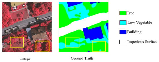
Figure 1.
Interclass similarity and fuzzy boundary (yellow rectangle box) of categories “Low Vegetable’’ and “Tree’’ in ISPRS Vaihingen dataset.
Semantic segmentation network with superior performance is the key to improve the accuracy of vegetation segmentation, and the core of improving performance is to search for more powerful feature representation. Therefore, how to improve the ability of feature representation is one of the challenges of the current work. The early image segmentation algorithms mainly extract the low-level features of the image for segmentation [10], and the segmentation results often do not contain semantic information. With the development of deep learning, a series of network models based on Convolutional Neural Networks (CNNs) [11] have been proposed successively and have entered a new stage of semantic segmentation. CNNs have powerful feature extraction ability and show superior performance in semantic segmentation tasks. However, CNNs capture local context information and pay little attention to the correlations among features that help in the accurate inference of semantic information, which limits the feature representation capability of the model and affects the capture of the most salient properties of an image for a given task to some extent. Related research has shown that representations produced by models can be enhanced by integrating learning mechanisms into the network, which helps to capture spatial and channel correlations among features [12]. On this basis, more and more modified networks were proposed to model the correlation in the channel or spatial dimensions [13,14], and various learning mechanisms were proposed to focus on the significant attributes of an image [15]. While most of the previous models focused on improving the joint coding of spatial and channel information, there are relatively few studies on the parallel coding of spatial and channel modes. Furthermore, as the depth of the model increases, problems such as over-fitting and gradient disappearance may occur, so our proposed model is mainly presented to solve the above problems.
In general, to further improve the ability of feature representation and learn a deeper and stronger network, we attempt to encode the channel and spatial information from another perspective. We propose a new module to aggregate the features generated by encoding spatial information and channel information in parallel. Additionally, we combine the proposed module with the residual structure to solve the problems such as network degradation and gradient disappearance that may occur in deep networks. Furthermore, to improve the segmentation accuracy of surface vegetation, we combine the height information provided by DSM images with IRRG images to segment the categories “Low Vegetable’’ and “Tree’’ more accurately to a certain extent. Therefore, the squeeze and excitation residual network (SERNet) is proposed, and the main contributions of this paper are summarized as follows:
- We introduce two kinds of SERMs into the semantic segmentation network to recalibrate feature responses adaptively and aggregate global information of the channel and spatial dimensions in parallel. The RAM is embedded into the bottom of the network to focus on features that are more informative among the features extracted by the network.
- We introduce DSM data and IRRG data to focus on the segmentation of surface vegetation categories, which helps to obtain better segmentation results.
- We conduct multiple comparative experiments using different data combinations and different models on the ISPRS Vaihingen and Potsdam datasets [16] to prove the superiority of the model.
2. Related Work
This section briefly describes some semantic segmentation methods based on deep learning, mainly including the following two aspects: semantic segmentation methods and attention mechanisms.
2.1. Semantic Segmentation Methods
Existing semantic segmentation methods generally include traditional methods based on machine learning and contemporary methods based on deep learning. Many traditional methods use machine learning algorithms to extract features based on the color, texture and spatial location of objects for image segmentation, such as threshold [17], edge detection [18], and clustering [19], but the handcrafted features used in most traditional methods have some limitations in terms of feature representation capacity. To address this problem, many advanced methods based on deep learning have been proposed and widely used recently [20]. Among them, the classical convolutional neural network (CNN) is the pioneer and became the tool of choice for many image segmentation tasks in computer vision [21,22]. The basic building block of CNN is the convolution layer. In each convolution layer, a set of filters extract spatial information and channel information within the local receptive fields and fuse them to generate feature maps. Then, global features and hierarchical patterns are generated by applying sequential convolution layers with nonlinear functions and down-sampling operators. The fully convolutional network (FCN) [23] is the first successful end-to-end deep convolutional neural network (DCNN) of semantic segmentation, which replaces the fully connected layer with the convolution layer to output the feature maps. Then, the segmentation result is generated by an up-sampling operation. FCN-based methods generally include an encoder and a decoder, but the size of the feature map decreases continuously in the process of feature extraction, resulting in loss of image content and spatial location information, which weakens the representation capacity of the network. To solve this problem, some improvements have been made based on the encoder and decoder structures [24,25]. Among them, U-Net [26] and its variants [27,28,29] concatenate global feature maps and local feature maps through skip connection, which helps the network generate precise semantic prediction. The contextual information in remote sensing images is particularly important for the feature representation capacity of the semantic segmentation model. In order to fuse multi-scale information of images, some studies use improved convolution operations such as dilated convolution to expand the receptive field and improve the performance of semantic segmentation [30,31,32]. One such approach, the pyramid scene parsing network (PSPNet) [33], aggregates contextual information of different scales through the spatial pyramid pooling module to avoid the loss of information representing the relationships between different subregions. DeeplabV3 [34] applies atrous convolution to extract multi-scale information, and DeepLabV3+ [35] further adds an effective decoder module to improve segmentation boundary accuracy. For mining multi-scale features, Inception models [36] integrate local information with global information and introduce multi-scale features to improve the performance. Furthermore, VGGNets [37] show that increasing the depth of a network could significantly improve the capacity of representation. ResNets demonstrate that it was possible to learn considerably deeper and stronger networks through the use of identity-based skip connections [38,39], which help the network to transfer information directly between low and high levels and solve the gradient problem that may occur in deep networks.
Building on these works, in order to improve the feature representation ability of semantic segmentation models, many studies apply the attention mechanism to model the correlation between features and focus on the features that are more meaningful to the current task. For example, the squeeze-and-excitation network (SENet) [40] introduces a channel attention mechanism and brings significant improvements in performance by modeling the interdependencies between the feature maps, so that the network can automatically learn the importance of different channel features. Pyramid Attention Network (PAN) [41] selects precise features through a global attention module in the channel dimension. However, these methods do not consider the interrelation of features in the spatial dimension, so many modified networks are proposed to model the correlation in the channel or spatial dimensions and propose various attention mechanisms to capture those attributes of an image that are most significant, such as the convolutional block attention module (CBAM) [42] and the semantic segmentation network with Spatial and Channel Attention Version 2 (SCAttNet V2) [43]. In addition, the Dual Attention Network (DANet) [44] uses two self-attention modules to calculate the feature representation of each position by the weighted sum of all other positions, which can model the long-range context information. The Residual Attention Network [45] uses a self-attention mechanism to obtain the self-attention weight by calculating the autocorrelation matrix of feature maps, which achieves better performance. In addition, some works utilized multi-modal data, mainly 3D elevation data (DSM or nDSM), to assist the semantic segmentation of remote sensing images, improving the accuracy of semantic prediction [46,47].
2.2. Land Cover Segmentation of Remote Sensing Images
With the development of earth observation technology, as a means to obtain land cover information in a wide range, remote sensing has been widely used in the task of land cover segmentation. The use of remote sensing images for land cover segmentation is an earlier application of remote sensing in the field of land use and monitoring. At present, the land cover segmentation of remote sensing images mainly adopts machine learning methods represented by Random Forest and deep learning methods represented by CNNs. Deep learning methods automatically extract features of objects by building deep networks to obtain higher segmentation accuracy. Penatti et al. [48] showed that CNNs vastly outperform the classical machine learning methods in terms of land cover segmentation. In the land cover segmentation part of the DeepGlobe challenge [49], the ranking list was completely dominated by deep neural networks (DNNs) [50], which have become the mainstream methods for land cover segmentation research of remote sensing images.
Although remote sensing technology has become the most effective means to obtain land cover information because it can provide dynamic and rich data sources, the variety and complex background of remote sensing images often lead to high inter-class similarity and low intra-class diversities similarity, which results in blurred boundaries and the difficult identification of small-scale targets [51] in remote sensing image segmentation. To solve these problems, many studies have embedded Pyramid Pooling Module (PPM), Attention Mechanism (AM), and other blocks in deep networks to improve the ability of extracting features from complex scenes. However, these methods do not make full use of the spatial position information contained in the global features, so they are more suitable for the recognition of large-scale objects, while the recognition effect of small-scale objects is not ideal. Therefore, in the research of land cover segmentation based on remote sensing images, the current methods mostly combine feature extraction and feature fusion to gradually recover the detailed information of the image and improve the recognition ability of multi-scale features, representative networks include U-Net, FPN [52] and Swin [53], etc. For instance, FPN proposed an approach for automatic multi-class land segmentation based on a fully convolutional neural network of the FPN family. RAANet [54] constructed an improved residual ASPP, which obtains multi-scale semantic information by embedding an attention module and residual structure and achieving superior land cover segmentation results.
In addition, as one of the land cover types, the accurate segmentation of surface vegetation is of great significance for monitoring the dynamic changes in vegetation cover, grassland degradation, and forest health status evaluation [55]. The research on vegetation segmentation is mostly based on traditional machine learning methods, which require artificial selection of feature variables, but the selection of feature variables has a greater impact on accuracy and is not generalizable. While the semantic segmentation method based on deep learning has good robustness and segmentation performance, it can avoid the impact of feature selection on the accuracy. With the rapid development of deep learning in the field of image segmentation, neural networks have been gradually applied to vegetation extraction and have achieved good segmentation results. Many scholars have proposed relevant vegetation segmentation methods, among which the denoising autoencoder [56] combines the traditional autoencoding structure and ensemble neural network so that the model can learn the essential features of the input to improve the accuracy of vegetation segmentation. You Only Look Once version 3 (YOLOv3) [57] and the faster region-based convolutional neural network (Faster R-CNN) [58,59] focus on the rapid detection and extraction of vegetation, which has great advantages in speed and comprehensive performance. Moreover, the double input residual DeepLabv3plus network (DIR DeepLabv3plus) [60] is proposed to reduce the impact of shading on vegetation segmentation, which can effectively improve the accuracy of vegetation extraction under shadowy conditions. Due to the powerful feature extraction and feature representation ability, deep-learning-based methods are often more effective than other vegetation segmentation methods based only on pixels or vegetation categories.
3. Methods
In this section, we introduce the proposed SERNet and give detailed descriptions of the SERM and RAM modules.
3.1. Network Architectures
The overall architecture of the proposed SERNet is shown in Figure 2. We use two different inputs for semantic segmentation of the original category and vegetation category in ISPRS datasets.
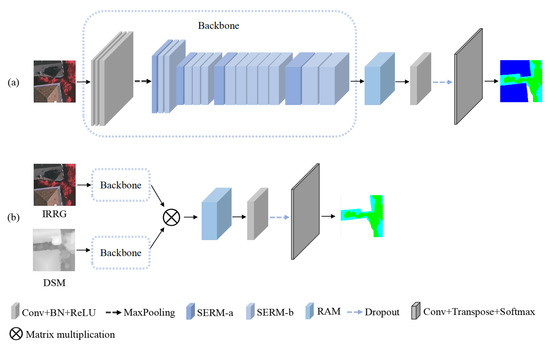
Figure 2.
SERNet Architecture. (a) SERNet with IRRG image as input, the convolution kernels of the first three modules are 3 × 3, the convolution kernel of the last module is 1 × 1, and the pool size of max pooling is 3 × 3. (b) SERNet with IRRG and DSM images as inputs.
3.1.1. Squeeze and Excitation Residual Network
As shown in Figure 2a, SERNet is based on ResNet and consists of two major parts: stacked SERMs for feature extraction and a RAM for better feature reconstruction. The SERM is composed of squeeze and excitation block (SE Block) and residual structure. In addition, for input HRRSIs, feature extraction is carried out by the deep network consisting of several SERMs. Afterward, the extracted features are fed into the RAM to enhance beneficial features. Then, semantic segmentation results are obtained through transposed convolution and softmax operations.
3.1.2. Segmentation of Surface Vegetation
Because of the similarity of the color and texture between the two categories “Low Vegetable” and “Tree” and the fuzzy boundary, the segmentation result is not very accurate. To this end, we add height information of DSM images in the feature extraction process. As shown in Figure 2b, IRRG images and DSM images in ISPRS datasets are extracted through the backbone of SERNet separately. Here, we make simple processing of the original labels, and merge categories other than “Low Vegetable” and “Tree” into the category “Background’’ to focus on the segmentation effect of “Low Vegetable” and “Tree”. The extracted feature maps are then fused through concentrate operation, the RAM is used to focus on the meaningful features, and the prediction results are obtained after transposed convolution and softmax operations.
3.2. Squeeze and Excitation Residual Module
The structures of the SE Block and two kinds of SERMs are depicted in Figure 3 and Figure 4. We introduce two new architectural units termed as: SERM-a and SERM-b, which insert SE Block into two kinds of regular residual structures. The SE Block consists of channel squeeze and excitation block (CSE Block) and spatial squeeze and excitation block (SSE Block), to improve the capacity of feature representation via modeling the interdependencies in the channel and spatial dimensions. We propose a mechanism that places the SE Block into two kinds of residual structures to perform feature recalibration adaptively, and the high-quality features can be spread smoothly in the deep network at the same time. Problems that might occur such as network degradation or vanishing gradient can be avoided in a certain way. In the notation that follows, we define the input feature maps . Here H, W, and C represent the height, width, and channels of the input feature maps, respectively, and the subscript c is the cth channel.
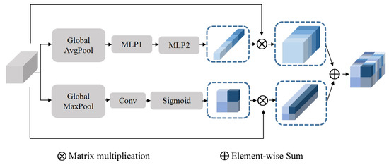
Figure 3.
Squeeze and Excitation Block. The dimensions of input and output are consistent.

Figure 4.
Squeeze and Excitation Residual Modules. The first line is SERM-a, the number of output channels is twice the number of input channels, and the second line is SERM-b.
3.2.1. Channel Squeeze and Excitation Block
The feature maps X are first passed through CSE Block, which models the interdependencies between the channels. Firstly, a multi-channel descriptor is produced by encoding feature maps across spatial dimensions, this descriptor is used to aggregate global information and transmitted at subsequent layers of the network. It is implemented by a global average pooling layer and generates the feature distribution of channel dimension, then producing vector Z with its elements by shrinking X through its spatial dimensions and using to denote a collection of channels of input feature maps .
After this, a simple mechanism is adopted to successively feed the multi-channel descriptor Z into two shared multilayer perceptrons with hidden layers to generate a set of modulation weights for each channel, and we use to denote the number of the hidden layer units is and , respectively. The generated modulation weights V are applied to the feature maps X through multiply operation to obtain the result of the CSE Block . The formula is shown in the following equation:
where the and represent two shared multilayer perceptrons, and ‖ represents concatenate operation.
3.2.2. Spatial Squeeze and Excitation Block
Similarly, SSE Block models the relationship between elements of the same spatial position in the input feature maps X and generates the feature distribution of spatial dimension. Furthermore, the spatial information is extremely effective for the deep network, while the distribution is complicated in HRRSIs and the size of ground objects varies greatly, especially for fine-grained image segmentation. To extract more recognizable spatial information and aggregate spatial feature maps across channel dimensions effectively, we use a global max pooling to obtain a feature tensor . Here, we use to denote a collection of the spatial position of the cth input feature map, and , . The superscript is the ith row and the jth column, and is the maximum value among the elements of and .
Then, the spatial feature recalibration is achieved through a reshape operation on M and a convolution operation with weight , and we generate a set of modulation weights . Finally, the result S is applied to the feature map X and passes through a sigmoid layer to recalibrate and excite X spatially. Then we can obtain the output of SSE Block :
where the ‖ represents concatenate operation, and · represents convolution operation.
3.2.3. Squeeze and Excitation Residual Block
We combine the channel and spatial information by an addition operation on the outputs of CSE Block and SSE Block, the generated feature of the SE Block is denoted as . On this basis, we insert it between the addition and the activation operations of the two residual structures shown in Figure 4. The SERMs parallelly encode spatial information and channel information and enable deep SERNet to avoid gradient problems and network degradation to a certain extent. Additionally, the extracted features are more global with the increasing depth of the network, SERM-a changes the dimension of the feature vector accordingly. The following SERM-b are connected in series, and the dimensions of input and output are the same.
3.3. Refine Attention Module
The RAM is constructed to focus on the more beneficial features to reconstruct the segmentation images accurately. For the extracted feature maps X that are generated by the deep layers, we feed them into the max pooling layer and average pooling layer; afterwards, two kinds of aggregating feature distributions are generated. To take advantage of the feature distributions, we employ a convolution operation with a set of weights and a sigmoid layer to generate U, then combine it with feature maps X through multiply operation. Finally, we can obtain the prediction results by transposed convolution and softmax operations. The structure is shown in Figure 5 and the formula for generating U is shown in the following equation:
where the and represent average pooling and max pooling, respectively, ‖ represents concatenate operation, and represents sigmoid.

Figure 5.
Attention Module. The kernel size of the convolution is 7 × 7.
4. Experiments
In this section, we briefly describe the datasets, evaluation metrics, and implementation details and verify the superiority of the proposed SERNet over other classic segmentation models through multiple sets of experiments. Firstly, IRRG images in ISPRS datasets are used to obtain segmentation results of different models, and the model performance is analyzed according to the results. Secondly, we verify the positive effect of introducing DSM images in helping the model achieve better results in vegetation segmentation.
4.1. Datasets
For ground object segmentation and surface vegetation segmentation, we use the original ISPRS dataset and the ISPRS dataset with labels processed into three categories.
4.1.1. Original Datasets
We evaluate the proposed model on ISPRS Vaihingen and Potsdam datasets provided by the International Society for Photogrammetry and Remote Sensing (ISPRS), which contains the high-resolution True Ortho Photo (TOP), Digital Surface Model (DSM), and ground truth images. The ground truth images are annotated according to six types: impervious surfaces, low-vegetation, cars, trees, buildings, and backgrounds.
The ISPRS Vaihingen dataset contains 33 true orthophoto images, 16 images with corresponding labels are used for training, and the remaining 17 images are used for testing. The resolution of the image is 9 cm, and the average size is 2064 × 2494. Moreover, each image includes three channels: near-infrared (NIR), red (R), and green (G). The ISPRS Potsdam dataset contains 38 orthophoto images, 24 images with corresponding labels are used for training, and the remaining 14 images are used for testing. The resolution of the image is 5 cm, and the size of each image is 6000 × 6000. In addition to the above three bands, it also contains blue (B). The categories are consistent with the ISPRS Vaihingen dataset.
For the ISPRS Vaihingen dataset, the accessible data are 16 pairs of original images and labeled images. We crop the images into pieces of size 256 × 256, and the training set and testing set are randomly divided from all available pieces in a ratio of 80%:20%. Due to the large original size of the ISPRS Potsdam dataset, IRRG images are used and we crop the 24 pairs of original images and labeled images into bigger patches with a size of 512 × 512. The training set and testing set are randomly divided from all available pieces in a ratio of 80%:20%.
4.1.2. Processed Datasets
In order to focus on the segmentation effect of the categories “Low Vegetable” and “Tree”, we process the label images of the ISPRS datasets and merge the categories “Impervious Surfaces’’, “Cars’’, and “Buildings’’ into the category “Background’’; then, only three categories are left in the merged label images. In addition, the cropping and division methods are consistent with those described above.
Both datasets provide corresponding DSM data generated from the original images by dense matching using the Match-T software [61]. The true orthophoto data and DSM data are defined on the same grid with consistent ground resolution. A part of the area covered by the DSM grid does not contain any data. In the DSM, these void areas are marked with a specific height value, and small void areas were filled using a variant of nonlinear diffusion that is adaptive to height changes [62]. We cropped the DSM images corresponding to ISPRS Vaihingen dataset to 256 × 256 and the DSM images corresponding to ISPRS Potsdam dataset to 512 × 512.
4.2. Evaluation Metrics
The semantic segmentation model is evaluated based on the confusion matrix of pixels, the confusion matrix represents the record of the true values and the predicted values, where the rows of the matrix represent the true value and the columns of the matrix represent the predicted value. The True Positives (TP) and the True Negative (TN) are the elements on the main diagonal, the False Positives (FP) are the accumulation of each column, excluding the main diagonal elements, while the False Negative (FN) is along the row. To evaluate the semantic segmentation results of the networks, we adopt three evaluation metrics, including mean intersection over union (mIoU), average F1-score (AF), and overall accuracy (OA). These metrics are defined as follows:
where N is the number of categories. is evaluated over a whole image, while and are evaluated for a specific class. and are evaluated for all categories as the averages of and , respectively.
Implementation Details
We train all the models from the scratch without using pre-training parameters and models. The parameter settings on the Vaihingen and Potsdam datasets are consistent during training: the batch size is set to 4, the learning rate is set to 1, and the Adam optimizer is adopted. We implement all the experiments on the Keras platform with an NVIDIA Tesla V100 GPU. Moreover, considering the distribution of dataset categories, we use the dice function to solve the class imbalance problem of the inputs and enforce a smooth training using cross entropy. Therefore, the combo loss [63] is adopted as the loss function, it is the weighted sum of modified cross entropy (C) and dice loss (D). The relevant formulas are as follows:
where and represent the predicted value and the true value, respectively; controls the amount of dice term contribution in the combo loss function ; and controls the level of model penalization for FP and FN. N is the product of the number of categories and number of samples. In our implementation, the value of and are both set to 0.5. To prevent division by zero, we set a smoothing factor S, and the value of S is set to 1.
4.3. Analysis
4.3.1. Segmentation of Original Categories
To evaluate the proposed SERNet framework, we compare the performance with the classic models shown in Table 1 and Table 2 on ISPRS Vaihingen and Potsdam datasets, which include the FCN-32s [23], FCN-8s [23], UNet [26], ResNet50 [38], RefineNet [28], CBAM [42], ResUNet++ [64], SCAttNet V2 [43], PSPNet [33], FPN [52], Deeplab v3+ [35], RAANet [54], and SENet [40]. We do not evaluate the category “Background” due to the fewer backgrounds in the ISPRS datasets.

Table 1.
Experimental results of original categories segmentation on the ISPRS Vaihingen dataset. The accuracy of each category is assessed by the IOU/F1-Score. Boldface indicates the best performance.

Table 2.
Experimental results of original categories segmentation on the ISPRS Potsdam dataset. The accuracy of each category is assessed by the IOU/F1-Score. Boldface indicates the best performance.
Table 1 shows the results of different models on the ISPRS Vaihingen dataset. It can be seen that among the three selected evaluation metrics mIoU, AF, and OA have achieved 72.69%, 84.49%, and 88.19% accuracy, respectively. Among the remaining models, SENet obtains the highest segmentation accuracy, the mIoU, AF, and OA are increased by 2.10%, 2.11%, and 2.44% respectively compare with SENet, which shows the effectiveness of the SERNet in extracting the category-based information. Table 2 shows the experimental results on the ISPRS Potsdam dataset, SERNet can produce 76.76% in mIoU, 87.04% in AF, and 90.29% in OA. Compared with SENet with the second highest results, the mIoU, AF, and OA are improved by 1.98%, 1.39%, and 2.38%, respectively. From Table 1 and Table 2, it can be clearly seen that our proposed SERNet is more accurate than other methods in terms of the segmentation accuracy for the categories “Imperious Surface”, “Building”, and “Car”, and the overall performance of SERNet is superior to other comparison methods. However, the best results are not obtained in the categories "Low Vegetable" and “Tree”. We also note the segmentation accuracy of these two categories is generally not ideal on all models. We think it is mainly because the small interclass variance between these two categories, such as color, texture, and other aspects, show high similarity, which brings great challenges to accurate semantic segmentation. In addition, the vegetation is widely distributed, with divergent and irregular edges and fuzzy boundaries. The proposed network has room for improvement in accurately segmenting irregular edges, and it is difficult to identify scattered objects belonging to these categories.
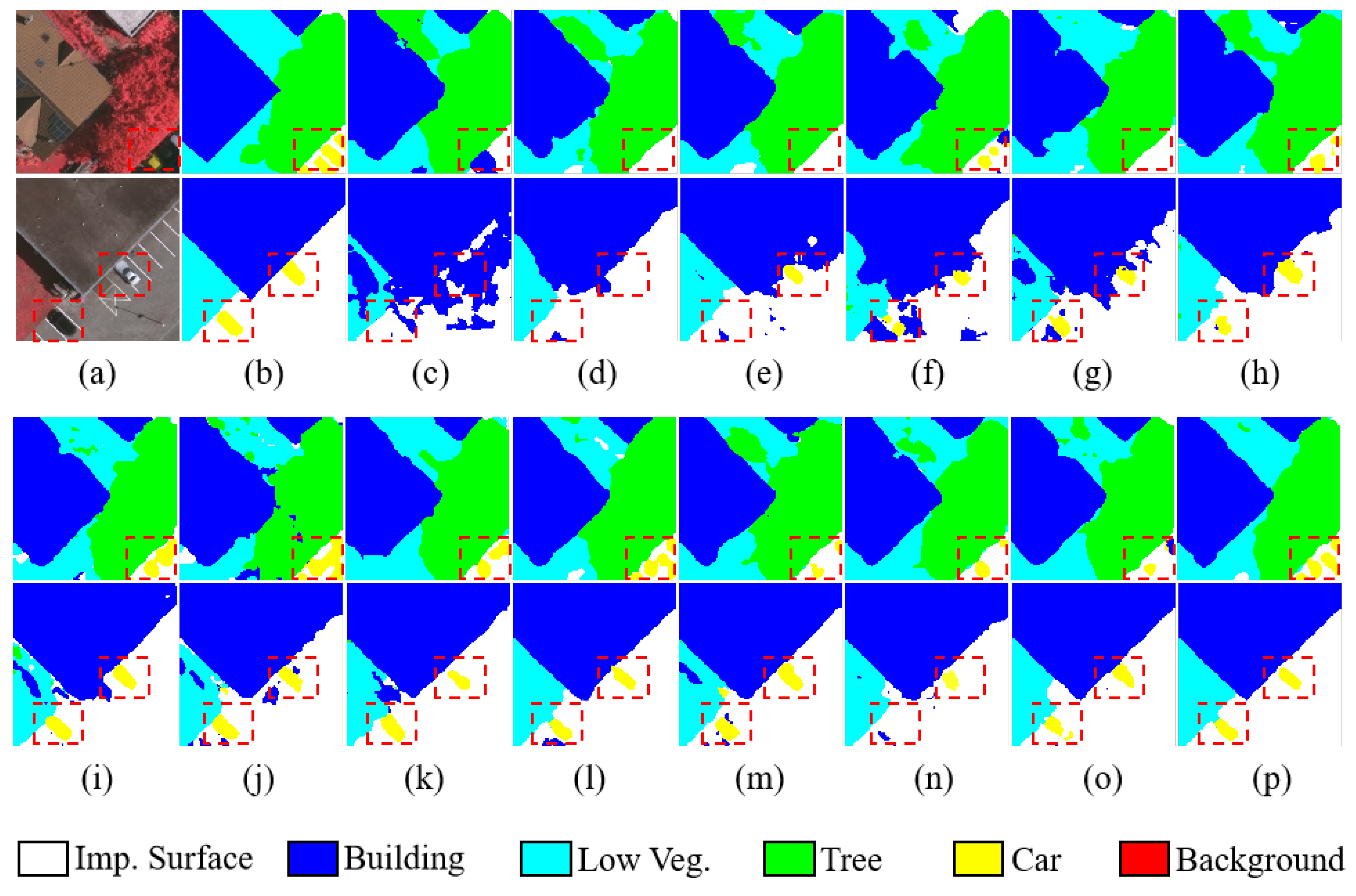
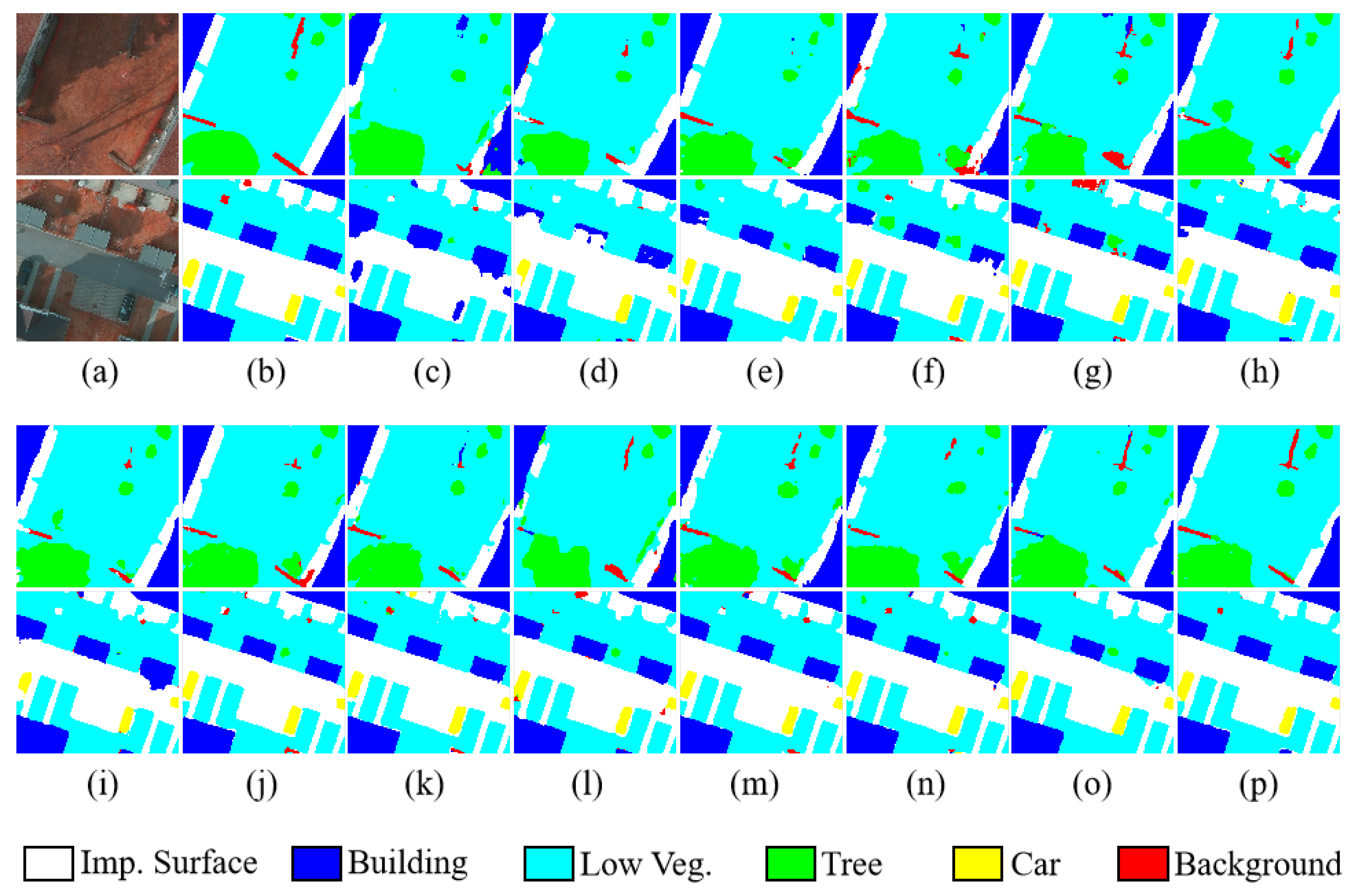
To display the segmentation results of the above models more visually, we visualize the original images, ground truth, and prediction results. In Figure 6 and Figure 7, it can be seen that the overall performance of SERNet is superior to other comparison methods and the boundaries among different classes are clearer. In addition, we can see from the red dashed box marked in Figure 6 that our model has obvious superiority for segmenting the small-size target category “Car”, and for the segmentation of large-size target categories such as “Building”, the edges are smoother.
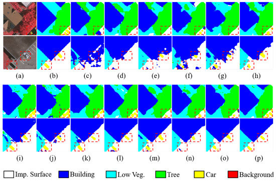
Figure 6.
Visualization results of the ISPRS Vaihingen dataset. (a) Original image. (b) Ground truth. (c) FCN-32s. (d) FCN-8. (e) UNet. (f) RefineNet. (g) ResNet50. (h) CBAM. (i) ResUNet++. (j) SCAttNet V2. (k) PSPNet. (l) FPN. (m) Deeplab v3+. (n) RAANet. (o) SENet. (p) SERNet.
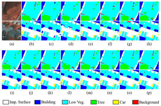
Figure 7.
Visualization results of the ISPRS Potsdam dataset. (a) Original image. (b) Ground truth. (c) FCN-32s. (d) FCN-8. (e) UNet. (f) RefineNet. (g) ResNet50. (h) CBAM. (i) ResUNet++. (j) SCAttNet V2. (k) PSPNet. (l) FPN. (m) Deeplab v3+. (n) RAANet. (o) SENet. (p) SERNet.
4.3.2. Segmentation of Vegetation Categories
To improve the segmentation accuracy of the categories “Low Vegetable” and “Tree”, we train all the models using the processed datasets which are merged into three categories. The results are shown in Table 3 and Table 4, and it can be seen that the segmentation results obtained with the processed datasets have improved compared with the original dataset on the three evaluation indicators we select, but the accuracy of each category has not improved that much. We consider that this is because the merger of categories improves the segmentation accuracy of the category “Background” while reducing the overall classification error; thus, the segmentation results appear to have a large improvement in OA. However, in fact, there is no significant impact on the vegetation segmentation that we focus on. The experimental results obtained by using only DSM images as input are shown in SERNet(A-DSM) in Table 3. DSM images train the feature representation ability of the model to a certain extent, and the elevation information provided by DSM images can achieve approximate segmentation of target categories, so we introduce DSM images to provide the elevation information and use the structure shown in Figure 2b to train SERNet with DSM images and IRRG images. As can be seen from the segmentation results in the penultimate line and the last line of Table 3 and Table 4, both vegetation category accuracy and overall accuracy have been significantly improved. Table 3 shows the results of different models on the ISPRS Vaihingen dataset. It can be seen that the mIoU, AF, and OA have achieved 76.85%, 87.29%, and 91.45%, respectively. Compared with SERNet(a), which only uses IRRG images as input, the mIoU, AF, and OA are improved by 1.45%, 1.90%, and 1.44%, respectively. Table 4 shows the experimental results on the ISPRS Potsdam dataset. SERNet(b) can produce 74.05% in mIoU, 85.66% in AF, and 92.59% in OA. Compared with SERNet(a), the mIoU, AF, and OA are improved by 1.53%, 1.61%, and 1.56%, respectively.

Table 3.
Experimental results of vegetation segmentation on the ISPRS Vaihingen dataset. The accuracy of each category was assessed by the IOU/F1-Score. Boldface indicates the best performance.

Table 4.
Experimental results of vegetation segmentation on the ISPRS Potsdam dataset. The accuracy of each category was assessed by the IOU/F1-Score. Boldface indicates the best performance.
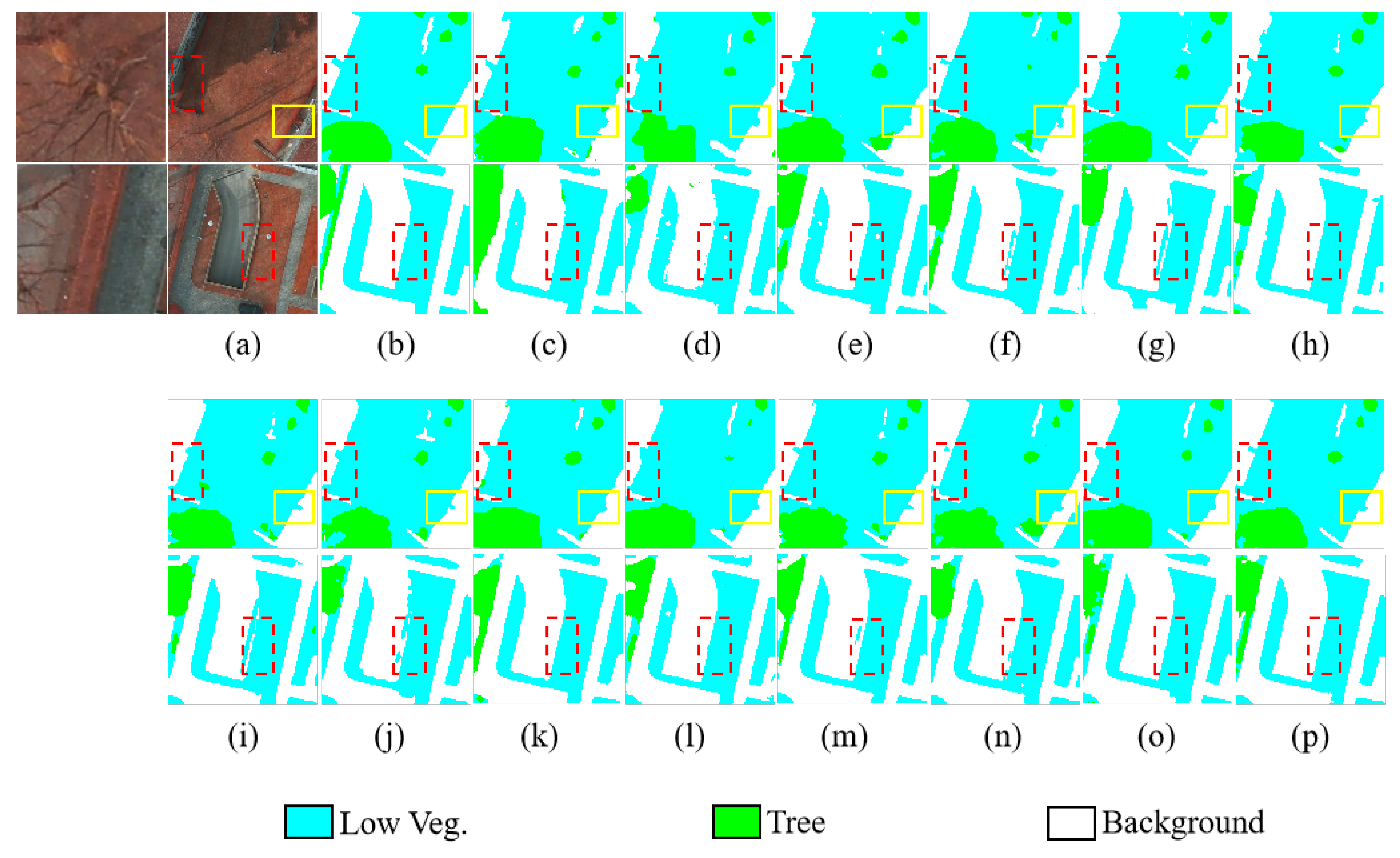
To show the vegetation segmentation results more intuitively, we visualize the original images, ground truth, and prediction results as shown in Figure 8 and Figure 9. We observed from the red dashed box in Figure 9 that the boundary between different categories is clearer and smoother in the segmentation result of SERNet(b). In addition, the segmentation results of object categories with random distribution and irregular shapes are more accurate. In particular, we find some of the same incorrect predictions among the several segmentation results. By comparing these visualization results with the real situation on the ground, we found that there is a small number of labeling errors in the ISPRS dataset, as shown by the areas with yellow rectangles in Figure 8 and Figure 9, and these incorrect prediction results actually correct the labeling errors in the original ISPRS datasets.
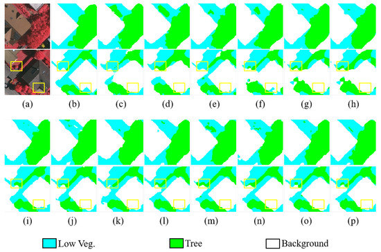
Figure 8.
Visualization results of the ISPRS Vaihingen dataset. (a) Original image. (b) Ground truth. (c) FCN-32s. (d) FCN-8. (e) UNet. (f) RefineNet. (g) ResNet50. (h) CBAM. (i) ResUNet++. (j) SCAttNet V2. (k) PSPNet. (l) FPN. (m) Deeplab v3+. (n) RAANet. (o) SENet. (p) SERNet.
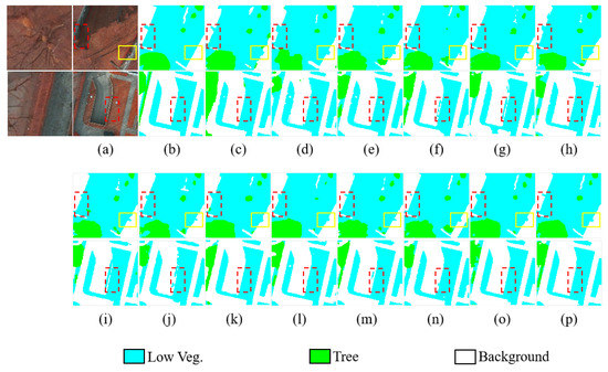
Figure 9.
Visualization results of the ISPRS Potsdam dataset; the left side of (a) shows an enlarged image of the main part of the “Tree” category in the original image. (a) Original image. (b) Ground truth. (c) FCN-32s. (d) FCN-8. (e) UNet. (f) RefineNet. (g) ResNet50. (h) CBAM. (i) ResUNet++. (j) SCAttNet V2. (k) PSPNet. (l) FPN. (m) Deeplab v3+. (n) RAANet. (o) SENet. (p) SERNet.
5. Discussion
5.1. Ablation Study
We also conducted an additional ablation experiment on the Vaihingen dataset to test the effects of SE Block and RAM on segmentation results. The third to last line of Table 1 is the network without SE Block and RAM, the second to last line is the network with SE Block inserted only, and the last line is the proposed SERNet.
The third to last line and the second to last line are studies on SE Block. It can be seen that the insertion of SE Block improves the semantic segmentation results significantly, especially for “Imperious Surface” and “Car”. The mIoU, AF, and OA are increased by 1.49%, 1.29%, and 1.40%, respectively. We argue that the insertion of SEBlock can recalibrate feature responses adaptively by modeling the long-range dependencies in the channel and spatial dimensions. Then, effective information can be transmitted from the shallow layer to the deep layer based on the deep residual network, which improves the feature representation ability and helps obtain better segmentation results. Additionally, the combo loss function we use solves the problem of class imbalance to a certain extent, so the segmentation of small targets such as “Car’’ may have a better performance. The second to last line and the last line are studies on RAM. Although RAM has a little effect on the improvement of the model performance, it has a positive effect on the network, as the mIoU, AF, and OA are increased by 0.31%, 0.41%, and 0.41%, respectively. We consider that RAM focuses on the global information that is more meaningful to the current task, so it has a certain effect on improving the prediction accuracy. However, since it is inserted at the bottom of the network and does not participate in the feature extraction process of the deep network, it has little influence on the feature extraction ability of the model.
5.2. Improvements and Limitations
The model we propose focuses on modeling the relationship between features in the channel and spatial dimensions, and realizes information transmission in deep layers, thereby improving the feature representation ability of the model. In addition, we further focus on the segmentation of surface vegetation, integrating elevation information provide by DSM images to improve the segmentation accuracy of the categories “Low Vegetable” and “Tree” in ISPRS datasets. Experimental results prove that our model improves the segmentation accuracy of the target objects through the proposed method.
In addition, our models and experimental results also have certain limitations. On the one hand, we introduce DSM images to improve the accuracy of the surface vegetation segmentation, but a simple fusion method is used to combine the features of the DSM images and the IRRG images, which may result in feature redundancy and negative mutual influence. Next, we will explore more appropriate methods in feature fusion, so that the model can capture the information from the IRRG images and the DSM images more effectively, and improve the segmentation performance of HRRSIs. On the other hand, the number of parameters of SERNet is relatively large, which increases the computation burden in a certain way. Therefore, an attempt can be made to reduce the computation of the model without affecting the model performance.
6. Conclusions
In this paper, we propose a promising semantic segmentation network that can perform feature recalibration adaptively and improve the capacity of feature representation to make high-quality features spread smoothly in the network. Experimental results on the ISPRS Vaihingen and Potsdam datasets confirm the superiority of the proposed model. Moreover, we merge the label images of the ISPRS datasets into three categories, and the features of DSM images and IRRG images are extracted and fused by the proposed model to improve the segmentation accuracy of vegetation categories. A series of experiments show that although the predictions become more accurate as the model is further improved, it still benefits from the introduction of elevation information. Therefore, additional information can increase the upper limit of segmentation accuracy, which may be emphasized when more challenging remote sensing datasets are published in the future.
Author Contributions
Conceptualization, X.Z.; methodology, L.L., G.C. and X.Z.; resources, L.L. and W.J.; writing—original draft preparation, X.Z., D.D. and M.E.; writing—review and editing, X.Z., D.D., J.W., W.J., M.E. and L.L.; visualization, W.J., M.E. and X.Z. All authors have read and agreed to the published version of the manuscript.
Funding
This research was funded by the National Natural Science Foundation of China (32171777), the Central University Basic Research Fund of China (2572020AW48), and the Heilongjiang Province Applied Technology Research and Development Program Major Project (GA20A301). (Corresponding author: Linhui Li).
Data Availability Statement
We utilized two public 2D semantic labeling datasets, Vaihingen and Potsdam, provided by the International Society for Photogrammetry and Remote Sensing (ISPRS). The Vaihingen dataset is freely available at http://www2.isprs.org/commissions/comm3/wg4/2d-sem-label-vaihingen.html, accessed on 18 September 2022, and the Potsdam dataset is freely available at http://www2.isprs.org/commissions/comm3/wg4/2d-sem-labelpotsdam.html, accessed on 18 September 2022.
Acknowledgments
The authors want to thank the International Society for Photogrammetry and Remote Sensing for providing the public datasets as the experimental data in this study.
Conflicts of Interest
The authors declare no conflict of interest.
References
- Li, M.; Chen, Z. Superpixel-enhanced deep neural forest for remote sensing image semantic segmentation. ISPRS J. Photogramm. Remote Sens. 2020, 159, 140–152. [Google Scholar]
- Moser, G.; Serpico, S.B.; Benediktsson, J.A. Land-Cover mapping by Markov modeling of spatial–contextual information in very-High-Resolution remote sensing images. Proc. IEEE 2013, 101, 631–651. [Google Scholar] [CrossRef]
- Dechesne, C.; Mallet, C.; Le Bris, A.; Gouet-Brunet, V. Semantic segmentation of forest stands of pure species combining airborne lidar data and very high resolution multispectral imagery. ISPRS J. Photogramm. Remote Sens. 2017, 126, 129–145. [Google Scholar] [CrossRef]
- Kampffmeyer, M.; Salberg, A.B.; Jenssen, R. Semantic Segmentation of Small Objects and Modeling of Uncertainty in Urban Remote Sensing Images Using Deep Convolutional Neural Networks. In Proceedings of the IEEE Conference on Computer Vision and Pattern Recognition (CVPR), Las Vegas, NV, USA, 27–30 June 2016; pp. 1–9. [Google Scholar]
- Liu, Y.; Minh Nguyen, D.; Deligiannis, N.; Ding, W.; Munteanu, A. Hourglass-ShapeNetwork Based Semantic Segmentation for High Resolution Aerial Imagery. Remote Sens. 2017, 9, 522. [Google Scholar] [CrossRef]
- Srivastava, S.; Volpi, M.; Tuia, D. Joint height estimation and semantic labeling of monocular aerial images with CNNS. In Proceedings of the 2017 IEEE International Geoscience and Remote Sensing Symposium (IGARSS), Fort Worth, TX, USA, 23–28 July 2017; pp. 5173–5176. [Google Scholar] [CrossRef]
- Zheng, Z.; Zhong, Y.; Wang, J. Pop-Net: Encoder-Dual Decoder for Semantic Segmentation and Single-View Height Estimation. In Proceedings of the IGARSS 2019—2019 IEEE International Geoscience and Remote Sensing Symposium, Yokohama, Japan, 28 July–2 August 2019; pp. 4963–4966. [Google Scholar] [CrossRef]
- Qin, R.; Fang, W. A hierarchical building detection method for very high resolution remotely sensed images combined with DSM using graph cut optimization. Photogramm. Eng. Remote Sens. 2014, 80, 873–883. [Google Scholar] [CrossRef]
- Sun, W.; Wang, R. Fully Convolutional Networks for Semantic Segmentation of Very High Resolution Remotely Sensed Images Combined With DSM. IEEE Geosci. Remote Sens. Lett. 2018, 15, 474–478. [Google Scholar] [CrossRef]
- Gedeon, T.; Parker, A.E.; Campion, C.; Aldworth, Z. Annealing and the normalized N-cut. Pattern Recognit. 2008, 41, 592–606. [Google Scholar] [CrossRef]
- Krizhevsky, A.; Sutskever, I.; Hinton, G.E. ImageNet Classification with Deep Convolutional Neural Networks; Inc.: Red Hook, NY, USA, 2012; Volume 25. [Google Scholar]
- Jaderberg, M.; Simonyan, K.; Zisserman, A. Spatial transformer networks. Adv. Neural Inf. Process. Syst. 2015, 28. [Google Scholar] [CrossRef]
- Bell, S.; Zitnick, C.L.; Bala, K.; Girshick, R. Inside-Outside Net: Detecting Objects in Context With Skip Pooling and Recurrent Neural Networks. In Proceedings of the IEEE Conference on Computer Vision and Pattern Recognition (CVPR), Las Vegas, NV, USA, 27–30 June 2016; pp. 2874–2883. [Google Scholar]
- Newell, A.; Yang, K.; Deng, J. Stacked Hourglass Networks for Human Pose Estimation. In Proceedings of the Computer Vision—ECCV 2016, Amsterdam, The Netherlands, 11–14 October 2016; Springer International Publishing: Cham, Switzerland, 2016; pp. 483–499. [Google Scholar]
- Veličković, P.; Cucurull, G.; Casanova, A.; Romero, A.; Lio, P.; Bengio, Y. Graph attention networks. arXiv Prep. 2017, arXiv:1710.10903. [Google Scholar]
- Cramer, M. The DGPF Test on Digital Aerial Camera Evaluation—Overview and Test Design. Photogramm. Fernerkund. Geoinf. 2009, 11, 73–82. [Google Scholar]
- Yang, Y.; Hallman, S.; Ramanan, D.; Fowlkes, C.C. Layered object models for image segmentation. IEEE Trans. Pattern Anal. Mach. Intell. 2012, 34, 1731–1743. [Google Scholar] [CrossRef]
- Al-Amri, S.S.; Salem Saleh, N.V.K.; Khamitkar, S.D. Image segmentation by using edge detection. Int. J. Comput. Sci. Eng. 2010, 2, 804–807. [Google Scholar]
- Zheng, X.; Lei, Q.; Yao, R.; Gong, Y.; Qian, Y. Image segmentation based on adaptive K-means algorithm. EURASIP J. Image Video Process. 2018, 2018, 1–10. [Google Scholar] [CrossRef]
- Sang, Q.; Zhuang, Y.; Dong, S.; Wang, G.; Chen, H.; Li, L. Improved land cover classification of VHR optical remote sensing imagery based upon detail injection procedure. IEEE J. Sel. Top. Appl. Earth Obs. Remote Sens. 2020, 14, 18–31. [Google Scholar] [CrossRef]
- Cordts, M.; Omran, M.; Ramos, S.; Rehfeld, T.; Enzweiler, M.; Benenson, R.; Franke, U.; Roth, S.; Schiele, B. The cityscapes dataset for semantic urban scene understanding. In Proceedings of the IEEE Conference on Computer Vision and Pattern Recognition, Las Vegas, NV, USA, 27–30 June 2016; pp. 3213–3223. [Google Scholar]
- Noh, H.; Hong, S.; Han, B. Learning Deconvolution Network for Semantic Segmentation. In Proceedings of the IEEE International Conference on Computer Vision (ICCV), Santiago, Chile, 11–18 December 2015; pp. 1520–1528. [Google Scholar]
- Long, J.; Shelhamer, E.; Darrell, T. Fully convolutional networks for semantic segmentation. In Proceedings of the IEEE Conference on Computer Vision and Pattern Recognition, Boston, MA, USA, 7–12 June 2015; pp. 3431–3440. [Google Scholar]
- Volpi, M.; Tuia, D. Dense Semantic Labeling of Subdecimeter Resolution Images With Convolutional Neural Networks. IEEE Trans. Geosci. Remote Sens. 2017, 55, 881–893. [Google Scholar] [CrossRef]
- Audebert, N.; Le Saux, B.; Lefèvre, S. Beyond RGB: Very high resolution urban remote sensing with multimodal deep networks. ISPRS J. Photogramm. Remote Sens. 2018, 140, 20–32. [Google Scholar] [CrossRef]
- Ronneberger, O.; Fischer, P.; Brox, T. U-net: Convolutional networks for biomedical image segmentation. In Proceedings of the International Conference on Medical Image Computing and Computer-Assisted Intervention, Munich, Germany, 5–9 October 2015; Springer: Berlin/Heidelberg, Germany, 2015; pp. 234–241. [Google Scholar]
- Badrinarayanan, V.; Kendall, A.; Cipolla, R. SegNet: A Deep Convolutional Encoder-Decoder Architecture for Image Segmentation. IEEE Trans. Pattern Anal. Mach. Intell. 2017, 39, 2481–2495. [Google Scholar] [CrossRef] [PubMed]
- Lin, G.; Milan, A.; Shen, C.; Reid, I. Refinenet: Multi-path refinement networks for high-resolution semantic segmentation. In Proceedings of the IEEE Conference on Computer Vision and Pattern Recognition, Honolulu, HI, USA, 21–26 July 2017; pp. 1925–1934. [Google Scholar]
- Yue, K.; Yang, L.; Li, R.; Hu, W.; Zhang, F.; Li, W. TreeUNet: Adaptive Tree convolutional neural networks for subdecimeter aerial image segmentation. ISPRS J. Photogramm. Remote Sens. 2019, 156, 1–13. [Google Scholar] [CrossRef]
- Ghiasi, G.; Fowlkes, C.C. Laplacian Pyramid Reconstruction and Refinement for Semantic Segmentation. In Proceedings of the Computer Vision—ECCV 2016, Amsterdam, The Netherlands, 11–14 October 2016; Springer International Publishing: Cham, Switzerland, 2016; pp. 519–534. [Google Scholar]
- Bilinski, P.; Prisacariu, V. Dense Decoder Shortcut Connections for Single-Pass Semantic Segmentation. In Proceedings of the IEEE Conference on Computer Vision and Pattern Recognition (CVPR), Salt Lake City, UT, USA, 18–22 June 2018; pp. 6596–6605. [Google Scholar]
- Nogueira, K.; Dalla Mura, M.; Chanussot, J.; Schwartz, W.R.; dos Santos, J.A. Dynamic Multicontext Segmentation of Remote Sensing Images Based on Convolutional Networks. IEEE Trans. Geosci. Remote Sens. 2019, 57, 7503–7520. [Google Scholar] [CrossRef]
- Zhao, H.; Shi, J.; Qi, X.; Wang, X.; Jia, J. Pyramid scene parsing network. In Proceedings of the IEEE Conference on Computer Vision and Pattern Recognition, Honolulu, HI, USA, 21–26 July 2017; pp. 2881–2890. [Google Scholar]
- Chen, L.C.; Papandreou, G.; Schroff, F.; Adam, H. Rethinking atrous convolution for semantic image segmentation. arXiv 2017, arXiv:1706.05587. [Google Scholar]
- Chen, L.C.; Zhu, Y.; Papandreou, G.; Schroff, F.; Adam, H. Encoder-decoder with atrous separable convolution for semantic image segmentation. In Proceedings of the European Conference on Computer Vision (ECCV), Munich, Germany, 8–14 September 2018; pp. 801–818. [Google Scholar]
- Szegedy, C.; Vanhoucke, V.; Ioffe, S.; Shlens, J.; Wojna, Z. Rethinking the Inception Architecture for Computer Vision. In Proceedings of the IEEE Conference on Computer Vision and Pattern Recognition (CVPR), Las Vegas, NV, USA, 27–30 June 2016; pp. 2818–2826. [Google Scholar]
- Simonyan, K.; Andrew, Z. Very deep convolutional networks for large-scale image recognition. arXiv 2014, arXiv:1409.1556. [Google Scholar]
- He, K.; Zhang, X.; Ren, S.; Sun, J. Deep residual learning for image recognition. In Proceedings of the Proceedings of the IEEE Conference on Computer Vision and Pattern Recognition; Las Vegas, NV, USA, 27–30 June 2016, pp. 770–778.
- He, K.; Zhang, X.; Ren, S.; Sun, J. Identity mappings in deep residual networks. In Proceedings of the European Conference on Computer Vision, Amsterdam, The Netherlands, 8–16 October 2016; Springer: Berlin/Heidelberg, Germany, 2016; pp. 630–645. [Google Scholar]
- Hu, J.; Shen, L.; Sun, G. Squeeze-and-excitation networks. In Proceedings of the IEEE Conference on Computer Vision and Pattern Recognition, Salt Lake City, UT, USA, 18–22 June 2018; pp. 7132–7141. [Google Scholar]
- Li, H.; Xiong, P.; An, J.; Wang, L. Pyramid Attention Network for Semantic Segmentation. arXiv Prep. 2018, arXiv:1805.10180. [Google Scholar]
- Woo, S.; Park, J.; Lee, J.Y.; Kweon, I.S. Cbam: Convolutional block attention module. In Proceedings of the European Conference on Computer Vision (ECCV), Munich, Germany, 8–14 September 2018; pp. 3–19. [Google Scholar]
- Li, H.; Qiu, K.; Chen, L.; Mei, X.; Hong, L.; Tao, C. SCAttNet: Semantic segmentation network with spatial and channel attention mechanism for high-resolution remote sensing images. IEEE Geosci. Remote Sens. Lett. 2020, 18, 905–909. [Google Scholar] [CrossRef]
- Fu, J.; Liu, J.; Tian, H.; Li, Y.; Bao, Y.; Fang, Z.; Lu, H. Dual Attention Network for Scene Segmentation. In Proceedings of the IEEE/CVF Conference on Computer Vision and Pattern Recognition (CVPR), Long Beach, CA, USA, 15–21 June 2019; pp. 3146–3154. [Google Scholar]
- Wang, F.; Jiang, M.; Qian, C.; Yang, S.; Li, C.; Zhang, H.; Wang, X.; Tang, X. Residual Attention Network for Image Classification. In Proceedings of the IEEE Conference on Computer Vision and Pattern Recognition (CVPR), Honolulu, HI, USA, 21–26 July 2017; pp. 3156–3164. [Google Scholar]
- Marcos, D.; Volpi, M.; Kellenberger, B.; Tuia, D. Land cover mapping at very high resolution with rotation equivariant CNNs: Towards small yet accurate models. ISPRS J. Photogramm. Remote Sens. 2018, 145, 96–107. [Google Scholar] [CrossRef]
- Marmanis, D.; Schindler, K.; Wegner, J.; Galliani, S.; Datcu, M.; Stilla, U. Classification with an edge: Improving semantic image segmentation with boundary detection. ISPRS J. Photogramm. Remote Sens. 2018, 135, 158–172. [Google Scholar] [CrossRef]
- Penatti, O.A.; Nogueira, K.; Dos Santos, J.A. Do deep features generalize from everyday objects to remote sensing and aerial scenes domains? In Proceedings of the IEEE Conference on Computer Vision and Pattern Recognition Workshops, Boston, MA, USA, 7–12 June 2015; pp. 44–51. [Google Scholar]
- Demir, I.; Koperski, K.; Lindenbaum, D.; Pang, G.; Huang, J.; Basu, S.; Hughes, F.; Tuia, D.; Raskar, R. Deepglobe 2018: A challenge to parse the earth through satellite images. In Proceedings of the IEEE Conference on Computer Vision and Pattern Recognition Workshops, Salt Lake City, UT, USA, 18–22 June 2018; pp. 172–181. [Google Scholar]
- Huang, G.; Liu, Z.; Van Der Maaten, L.; Weinberger, K.Q. Densely connected convolutional networks. In Proceedings of the IEEE Conference on Computer Vision and Pattern Recognition, Honolulu, HI, USA, 21–26 July 2017; pp. 4700–4708. [Google Scholar]
- Neupane, B.; Horanont, T.; Aryal, J. Deep learning-based semantic segmentation of urban features in satellite images: A review and meta-analysis. Remote Sens. 2021, 13, 808. [Google Scholar] [CrossRef]
- Seferbekov, S.; Iglovikov, V.; Buslaev, A.; Shvets, A. Feature pyramid network for multi-class land segmentation. In Proceedings of the IEEE Conference on Computer Vision and Pattern Recognition Workshops, Salt Lake City, UT, USA, 18–22 June 2018; pp. 272–275. [Google Scholar]
- Liu, Z.; Lin, Y.; Cao, Y.; Hu, H.; Wei, Y.; Zhang, Z.; Lin, S.; Guo, B. Swin transformer: Hierarchical vision transformer using shifted windows. In Proceedings of the Proceedings of the IEEE/CVF International Conference on Computer Vision, Online, 11–17 October 2021; pp. 10012–10022. [Google Scholar]
- Liu, R.; Tao, F.; Liu, X.; Na, J.; Leng, H.; Wu, J.; Zhou, T. RAANet: A Residual ASPP with Attention Framework for Semantic Segmentation of High-Resolution Remote Sensing Images. Remote Sens. 2022, 14, 3109. [Google Scholar] [CrossRef]
- Coy, A.; Rankine, D.; Taylor, M.; Nielsen, D.C.; Cohen, J. Increasing the Accuracy and Automation of Fractional Vegetation Cover Estimation from Digital Photographs. Remote Sens. 2016, 8, 474. [Google Scholar] [CrossRef]
- Li, Y.; Cao, Z.; Xiao, Y.; Lu, H.; Zhu, Y. A novel denoising autoencoder assisted segmentation algorithm for cotton field. In Proceedings of the 2015 Chinese Automation Congress (CAC), Wuhan, China, 27–29 November 2015; pp. 588–593. [Google Scholar] [CrossRef]
- Liu, H.; Sun, H.; Li, M.; Iida, M. Application of Color Featuring and Deep Learning in Maize Plant Detection. Remote Sens. 2020, 12, 2229. [Google Scholar] [CrossRef]
- Xu, W.; Zhao, L.; Li, J.; Shang, S.; Ding, X.; Wang, T. Detection and classification of tea buds based on deep learning. Comput. Electron. Agric. 2022, 192, 106547. [Google Scholar] [CrossRef]
- Zhuang, S.; Wang, P.; Jiang, B. Segmentation of Green Vegetation in the Field Using Deep Neural Networks. In Proceedings of the 2018 13th World Congress on Intelligent Control and Automation (WCICA), Changsha, China, 4–8 July 2018; pp. 509–514. [Google Scholar] [CrossRef]
- Yang, L.; Chen, W.; Bi, P.; Tang, H.; Zhang, F.; Wang, Z. Improving vegetation segmentation with shadow effects based on double input networks using polarization images. Comput. Electron. Agric. 2022, 199, 107123. [Google Scholar] [CrossRef]
- Lemaire, C. Aspects of the DSM production with high resolution images. In Proceedings of the International Archives of the Photogrammetry, Remote Sensing and Spatial Information Sciences; 2008; Volume 37, pp. 1143–1146. Available online: https://www.isprs.org/proceedings/XXXVII/congress/4_pdf/200.pdf (accessed on 18 September 2022).
- Kosov, S.; Rottensteiner, F.; Heipke, C.; Leitloff, J.; Hinz, S. 3D Classification of Crossroads from Multiple Aerial Images Using Markov Random Fields. Int. Arch. Photogramm. Remote Sens. Spat. Inf. Sci. 2012, XXXIX-B3, 479–484. [Google Scholar] [CrossRef]
- Taghanaki, S.A.; Zheng, Y.; Zhou, S.K.; Georgescu, B.; Sharma, P.; Xu, D.; Comaniciu, D.; Hamarneh, G. Combo loss: Handling input and output imbalance in multi-organ segmentation. Comput. Med. Imaging Graph. 2019, 75, 24–33. [Google Scholar] [CrossRef]
- Jha, D.; Smedsrud, P.H.; Riegler, M.A.; Johansen, D.; De Lange, T.; Halvorsen, P.; Johansen, H.D. Resunet++: An advanced architecture for medical image segmentation. In Proceedings of the 2019 IEEE International Symposium on Multimedia (ISM), San Diego, CA, USA, 9–11 December 2019; pp. 225–2255. [Google Scholar]
Publisher’s Note: MDPI stays neutral with regard to jurisdictional claims in published maps and institutional affiliations. |
© 2022 by the authors. Licensee MDPI, Basel, Switzerland. This article is an open access article distributed under the terms and conditions of the Creative Commons Attribution (CC BY) license (https://creativecommons.org/licenses/by/4.0/).


