Abstract
The classification and quantification of fuel is traditionally a labour-intensive, costly and often subjective operation, especially in hazardous vegetation types, such as gorse (Ulex europaeus L.) scrub. In this study, unmanned aerial vehicle (UAV) technologies were assessed as an alternative to traditional field methodologies for fuel characterisation. UAV laser scanning (ULS) point clouds were captured, and a variety of spatial and intensity metrics were extracted from these data. These data were used as predictor variables in models describing destructively and non-destructively sampled field measurements of total above ground biomass (TAGB) and above ground available fuel (AGAF). Multiple regression of the structural predictor variables yielded correlations of R2 = 0.89 and 0.87 for destructively sampled measurements of TAGB and AGAF, respectively, with relative root mean square error (RMSE) values of 18.6% and 11.3%, respectively. The best metrics for non-destructive field-measurements yielded correlations of R2 = 0.50 and 0.49, with RMSE values of 40% and 30.8%, for predicting TAGB and AGAF, respectively, indicating that ULS-derived structural metrics offer higher levels of precision. UAV-derived versions of the field metrics (overstory height and cover) predicted TAGB and AGAF with R2 = 0.44 and 0.41, respectively, and RMSE values of 34.5% and 21.7%, demonstrating that even simple metrics from a UAV can still generate moderate correlations. In further analyses, UAV photogrammetric data were captured and automatically processed using deep learning in order to classify vegetation into different fuel categories. The results yielded overall high levels of precision, recall and F1 score (0.83 for each), with minimum and maximum levels per class of F1 = 0.70 and 0.91. In conclusion, these ULS-derived metrics can be used to precisely estimate fuel type components and fuel load at fine spatial resolutions over moderate-sized areas, which will be useful for research, wildfire risk assessment and fuel management operations.
Keywords:
fuel load; UAV; lidar; fuel classification; deep learning; semantic segmentation; biomass; shrubland 1. Introduction
With the onset of human-induced climate change, wildfires are growing in frequency and intensity. Wildfires in recent years have reached unprecedented levels in a number of countries, including the United States [1], Australia [2,3], Portugal [4] and Canada [5]. Over the past five years, Aotearoa New Zealand (NZ) has experienced some of the largest and most destructive wildfires in its history [6,7,8]. The destructive nature of these fires appears to be linked to an increase in the frequency of fires at the rural–urban interface, posing a greater threat to human life and property [6,9]. Shrubby environments comprise a considerable amount of the natural vegetation in heavily populated areas of many countries, including NZ [10] and shrub encroachment into other ecosystems poses a higher risk of wildfire [10,11]. Shrub encroachment is increasing globally for various reasons including climate change [12,13] and changes in grazing or agricultural practices [14,15], and as a response to the suppression of indigenous fire management practices [16]. As wildfires continue to grow in intensity and frequency, it is critical that scalable methods are developed in order to better measure the environmental variables that can be used to model, manage and suppress wildfires.
Vegetation management is in need of practical, accurate and scalable methods for vegetation inventory, including forest mensuration [17,18], fuel type mapping [19], risk evaluation for wildfire management [20,21] and habitat monitoring [22]. Traditional methods that are used for mapping fuel types and fuel properties based on field data collection can be costly and challenging [23,24]. Traditional methods can yield precise measurements for cover and biomass; however, they require labour-intensive and logistically challenging field work to collect data in a highly localized manner, which is not easily scalable [22]. This is especially true for vegetation communities consisting of spiny species that grow in dense masses, such as gorse (Ulex europaeus L.), offering additional challenges and hazards for field crews.
As an alternative to field-based fuel assessments, remote sensing offers multiple benefits, most notably the ability to capture objective, cost-efficient measurements over large, often isolated areas [25]. Remote sensing technologies have been demonstrated to be an effective method for estimating vegetation metrics such as biomass, structural properties and fuel loadings [23,26,27,28]. Spectral and spatial information can be retrieved from passive sensors mounted on airborne and spaceborne platforms [23]. Structural information can be retrieved from active sensors such as airborne laser scanning (ALS) or synthetic aperture radar (SAR) [29]. Arguably the best remote-sensing methods for retrieving vegetation structural information are ALS and terrestrial laser scanning (TLS) [30]. Although many studies have used ALS to predict forest fuel metrics [28,29,31,32,33,34,35,36,37], comparatively few have applied this technology in shrublands [38,39,40,41,42] and even fewer attempted to predict shrub fuel metrics [43]. The difficulty in applying ALS to describe vegetation properties in shrub environments lies in the structural homogeneity of low heights and relatively uniform canopy surface common to shrubland vegetation [23,44]. ALS is arguably more suited for characterising forest canopy structures than for characterizing low lying vegetation, such as understory or shrubland vegetation, owing to the low density of returns and the obstruction caused by taller canopy structures [45].
An alternative method of laser scanning that creates point clouds with a higher definition of vegetation surfaces is TLS. This method utilises a ground-based static laser scanner to create point clouds from a much closer range, leading to a greater point density, and smaller laser footprint. In combination, these features of TLS result in a more accurate representation of vegetation structure [46,47]. TLS has been used for a variety of forestry-related applications, including tree height measurement [48], biomass estimation [49], and extensively for forest mensuration and tree stem characterization [50]. This technology has been proven to be highly effective for the characterization of shrub environments without destructive sampling [46,51,52]. There is a discrete body of research building up around the application of TLS to fuel modelling [53,54,55]. Some of these published studies are focused on the efficacy of TLS for fuel load characterization in shrub ecosystems [45,56,57,58,59]. Although previous studies have observed good correlations between field and TLS measurements for cover and biomass [22,39,51], a common issue with TLS data is the presence of “shadows” in the point cloud. S Due to the stationary nature of the TLS system, shadows are caused when objects in the captured scene are occluded by other objects [22].
With the miniaturisation of airborne laser scanners, unmanned aerial vehicles (UAVs) are now a viable alternative for characterizing increasingly large areas with laser scanning technology [30]. UAV laser scanning (ULS) has been shown to be a highly effective tool for characterizing tree height, stem diameters and other individual tree metrics in forest environments [30,60,61]. As ULS has a higher point density and smaller laser footprint than ALS, ULS has the potential to accurately characterize more homogeneous environments, such as shrublands, by providing an enhanced definition of vegetation architecture [46]. It has been proposed that ULS could provide a useful tool to fill the void between the high-density yet small area coverage of TLS and the low-density, wide area coverage of ALS [57]. To date, very few studies have focused on the characterization of shrub environments using ULS [42,46,62]. Even fewer of these studies have focused on fuel modelling [36], and only one has used ULS to characterise shrub fuel [63].
As the type of fuel has a strong influence on fire behaviour [64], it is useful not only to characterise the fuel load but also to classify the fuel type. Previous studies have found that ALS alone is not effective for characterising the vegetation canopy of low vegetation [65]. Even at higher laser return densities, the structure of completely different vegetation types could look very similar in a laser-scanned point cloud. The utility of lidar for fuel characterisation has been supplemented through the addition of multispectral imagery from fixed-wing aircraft [65,66] and satellites [28,35].
Recent advances in the field of machine learning have led to the development of highly versatile deep learning models for the detection and classification of objects in images [67]. When combined with visual-spectrum UAV imagery, deep learning algorithms can be used to undertake fine-grained detection and classification for a wide range of vegetation-related applications. These applications include pest–plant detection [68,69], tree seedling detection [70] and the semantic segmentation of different vegetation types [71,72,73]. Semantic segmentation is the process of automatically assigning each pixel in the image to a specific class. The segmentation can either be single class, also referred to as binary segmentation, or multi-class segmentation, where the model can be trained to distinguish between multiple categories at the same time. Very little research has focused on deep learning semantic segmentation of UAV imagery for the classification of fuel types. Using high-resolution UAV orthomosaics, our objectives were to address this knowledge gap by classifying fuel components within a gorse scrub environment down to individual species and characterising their health status by discriminating live and dead vegetation.
The aims of this study were (1) to assess whether UAV orthomosaics combined with semantic segmentation through deep learning can be used to characterise fuel classes, (2) to assess whether metrics derived from ULS and UAV orthomosaic data can be used to accurately determine fuel load, and (3) to evaluate ULS as a viable alternative to non-destructive field measurements.
2. Materials and Methods
2.1. Study Site
Data for this study were collected as part of a large, multi-year fire research programme in Aotearoa New Zealand (NZ). The aim of this wider programme was to conduct heavily instrumented experimental field burns in a range of different vegetation types [74,75] from cereal crop stubble to shrubland vegetation and wilding conifer forests. The site for the shrubland burn experiments was located at ~345 m above sea level, between the base of Mount Hutt and the Rakaia River in Canterbury in the South Island of NZ (43°24′31″S, 171°34′01′′E; Figure 1). The terrain was flat with a slight NW to SE gradient of ~2 m, with thin soils over river rock. At this site, shrub vegetation has colonised a fluvial deposition alongside a meandering braided river. The Rakaia river site has been extensively colonised by gorse (Ulex europaeus L.), and to a lesser extent by the native shrub species matagouri (Discaria toumatou Raoul, matakoura or tūmatakuru in te reo Maori), dog rose (Rosa canina), various species of lupin (Lupinus spp.) and several species of native and exotic grasses. The shrub layer within the study site ranged from 0.2 to 2.0 m tall, with the site exhibiting heterogeneity in both height and density.
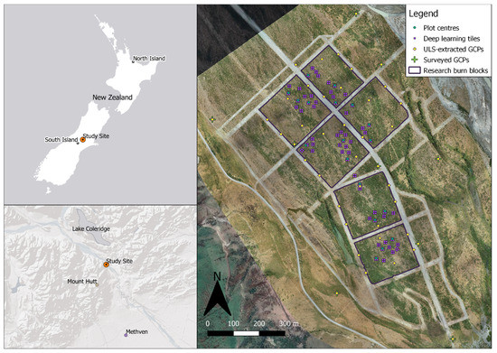
Figure 1.
Map of the study site showing location of GCPs, plots, deep learning tiles and burn blocks. Inset maps show the site location.
The study site sits within a cool wet hill climate with annual rainfall between 750–1500 mm and prevailing north-westerly winds [76]. Meteorological conditions were recorded on a temporary weather station that was installed on the site for the duration of the study. The mean daily temperature on the site during the study period ranged from 12.5 °C to 23.8 °C, with the mean daily relative humidity ranging between 53% and 83% and the mean daily wind speed ranging between 3.5 m/s and 11.9 m/s. No precipitation was observed during the study period. More detailed information on the ambient conditions of the site for the study period can be found in Appendix A, Table A1.
2.2. Field Sampling and Non-Destructive Measurements
Six 200 m × 200 m burn blocks were established across the site. These blocks were separated from each other by 10 m wide fire breaks, which were bulldozed and graded to prevent fire escape into the neighbouring shrubland. Within each of the six burn blocks, three 4 × 1 m fuel sampling quadrats were established (Figure 2). The quadrats were positioned so that the vegetation samples were representative of the range of vegetation across the burn blocks. This was determined by analysing previously sampled transects across the burn area. Each sampling quadrat was divided into four 1 × 1 m “sub-quadrats” aligned in a north to south orientation (Figure 2b). The method follows the methodology laid out in [24], with non-destructive fuel measurements being made within each sub-quadrat. The four sub-quadrats method maximises the variability in vegetation cover, which can be dominated by a single shrub in the larger 4 × 1 m quadrats. Once established, average height and cover measurements were determined for each of the vegetation components in the overstory, understory and litter strata present within the overall quadrat. Non-destructive sampling took place between the 10 and 14 February 2020.
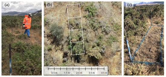
Figure 2.
(a) Field plot establishment; (b) digitised 4 × 1 m quadrat, showing the layout of the four 1 × 1 m sub-plots used for non-destructive sampling; (c) field plot after destructive sampling, showing the painted outline used for annotation in the GIS.
Heights for each of the vegetation strata were determined as the average height of the tallest and shortest clumps of fuel. Heights for isolated shrubs that clearly did not belong to the main fuel strata were disregarded. Overstory height (OsHt) for each quadrat was then calculated as the mean of the overstory measurements from each of the sub-quadrats. Percentage cover for each of the strata was visually estimated within each sub-quadrat, and overstory cover (OsCo) was calculated from a combination of the percentage cover of the woody overstory species such as gorse, matagouri and rose.
2.3. Destructive Sampling
Following the methodology described in [24], all vegetative material for each fuel component within each 4 × 1 m quadrat was destructively sampled, starting with the overstory layer and finishing with the litter layer. The vegetative material was separated by species, sorted as either live or dead based on colour and general appearance, and split into four groups based on diameter (≤0.49, 0.5–0.99, 1.0–2.99 and ≥3.0 cm) as described in [77]. Destructive sampling took place between 11 and 20 February 2020.
The wet weight of each fuel component was measured in the field using a hanging scale suspended from a 2 m tall metal frame, which provided a measurement of fresh biomass. Total above ground biomass (TAGB; kg/m2) was determined by drying samples in an oven at 105 °C for 24 h or 65 °C for 48 h for the heavier fuels >1 cm, thus removing all moisture. Depending on the amount of material in each fuel component, either the entire sample or a sub-sample of it was taken to the lab for drying. Above ground available fuel (AGAF) was determined using the smallest components of the elevated fuel, plus understory vegetation and litter. The elevated fuel component in the AGAF estimates included all (100%) of the dead and 81% of live foliage (i.e., gorse and matagouri) less than 0.5 cm, as per [24].
A total of eighteen 4 × 1 m plots were measured across the site; however, due to an outbreak of COVID-19, two of the samples were not able to be processed in time and were therefore discarded from the sample. The results from the destructive and non-destructive field measurements showed a wide range in quantitative and structural properties (Table 1), with maximum vegetation height ranging from 0.74 to 2.15 m and biomass ranging from 1.68 to 12.7 kg/m2.

Table 1.
Summary of destructive and non-destructive fuel characteristics of the field sample plots (n = 16).
2.4. UAV Data Acquisition
Prior to flight, an extensive network of ground control points (GCPs) was set up across the site to geolocate the UAV data for lidar and Structure from Motion (SfM) captures. GCPs were surveyed prior to the data capture using a handheld Trimble Geo7X GPS unit (Trimble Inc., Sunnyvale, CA, USA) combined with a Trimble Zephyr Model 2 external aerial (Trimble Inc., Sunnyvale, CA, USA). To attain a GPS fix at the centre of each point, an average was taken from a minimum of 180 point fixes over approximately 3 min.
Nine GCPs were established across the site to increase the accuracy of the lidar, with minimum, maximum and average RMSE values of 0.03 m and 0.28 m and 0.15 m, respectively. An additional point was surveyed in the centre of the area of interest utilising the same method as described above to be used as the base station location for the UAV lidar system. Surveying of this point collected 600 points averaged over 10 min, and the resulting RMSE for this point was 0.18 m.
For the photogrammetry, a further 32 GCPs were established across the site. In total, 41 GCPs were installed with a maximum spacing of ~100 m between GCPs (Figure 1), which resulted in a vertical RMSE for the photogrammetric data of less than 0.1 m [78]. The distribution of the points was planned to reduce potential errors in the photogrammetry, such as bowl effect [79]. Point fixes for photogrammetric GCPs were obtained from the ULS-derived digital terrain model (DTM) to reduce survey time. High-contrast photogrammetric plates were deployed to increase their visibility in the point cloud.
The ULS dataset capture was carried out using a LidarUSA Snoopy V-series system (Fagerman Technologies, INC., Somerville, AL, USA), with an integrated Riegl MiniVUX-1 UAV scanner (Riegl, Horn, Austria). The LidarUSA system, hereafter referred to as the MiniVUX, was carried by a DJI Matrice 600 Pro UAV (DJI Ltd., Shenzhen, China). A Zenmuse X4s (DJI Ltd., Shenzhen, China) 1-inch 20 MP RGB camera mounted on a DJI Matrice 210 (DJI Ltd., Shenzhen, China) was used to capture all SfM data.
Flight planning for the ULS capture was undertaken using UgCS software version 3.4 (SPH Engineering, Riga, Latvia). This software can program adaptive banking turns into the flight path, thereby reducing the accumulation of error in the scanner’s IMU position during flights. For the photogrammetry flights, the Map Pilot (Drones Made Easy, San Diego, CA, USA) application was utilised as it has in-built terrain-following functionality that ensured an even flight altitude and, therefore, even ground sample distance (GSD) across images. SfM datasets were captured before and after destructive sampling to map the vegetation across the site and to enable accurate annotation of plot locations in the GIS (see Section 2.6). Plot-level SfM datasets were captured at a higher resolution to evaluate the full potential of a deep learning approach. Flight parameters and data resolution statistics for the various captured datasets are given in Table 2.
Table 2.
Flight parameters and data resolution statistics for UAV data captures.
Following Dandois et al. [80], UAV data were captured under clear sky conditions, during periods of high solar angle, on days with wind speeds lower than 20 km/h, thereby minimising blur and shadow in the imagery. Whole site operations were planned with a ground sample distance (GSD) of ~3.5 cm, a speed that kept motion blur between less than 1 × the GSD (recommendations in the literature vary between <0.5 and <1.5 times the GSD [81,82]) and a minimum forward and side overlap of 80% [80]. For the high resolution photogrammetric flights, side and forward overlap was increased to 85% to reduce potential artefacts in the outputs resulting from the complex structure of the vegetation [83]. Site-level SfM datasets were captured on 6 February and 1 March 2020, with plot-level SfM datasets captured on 7 February 2020.
For the lidar flights, a line spacing of 30 m and a speed of 5 m/s were selected to create a very high density point cloud, to ensure maximum coverage of the vegetation. In line with flight parameters used in a previous study, which reported a correlation and accuracy of R2 = 0.99 and RMSE = 0.15 m for tree height [60], a flight height of 50 m AGL was selected. This also maintains a small laser beam footprint (80 × 25 mm at 50 m) and, therefore, lowers the error with a reported accuracy for the MiniVUX of 0.015 m at 50 m [84]. The ULS dataset was captured on 7 February 2020.
2.5. Raw Data Processing
2.5.1. ULS
To generate a point cloud in the universal LAS format, raw lidar data were retrieved from the sensor and converted from the sensor’s native LidarUSA format in two processing steps. First, the Inertial Explorer Xpress software version 8.90 (NovAtel Inc., Calgary, AB, Canada) was used to post-process the raw trajectory data from the GNSS rover of the LidarUSA system with the post-processed kinematic (PPK) GPS data from the CHCX900B base station (CHC Navigation, Shanghai, China). PPK processing increases the accuracy of the trajectory data. The ScanLook Point Cloud Export (ScanLook PC) software version 1.0.230 (Fagerman Technologies INC., Somerville, AL, USA) was then utilised to combine the post-processed trajectory data with the raw sensor data from the MiniVUX. ScanLook PC was also used to apply the boresight calibrations and lever arm offsets that are unique to the sensor and how it was mounted on the craft. This process removed inherent errors associated with mismatched data from within or between flight lines. The resulting point cloud was then output in the universal LAS format. LAS was preferable to the LAZ format as, being uncompressed, it could be read faster and therefore reduced the processing time and aided in parallelisation during the next processing steps.
2.5.2. Orthomosaic
Pix4Dmapper (Pix4D) software version 4.7.5 (Pix4D, Lausanne, Switzerland) was used to process the UAV imagery into orthomosaics. The image processing in Pix4D followed three general stages: (1) initial processing; (2) point cloud mesh generation; and (3) DSM (digital surface model), orthomosaic and index generation. Upon completion of stage 1, 3D GCPs were added to the project for enhanced spatial reference. In order to create a good orthomosaic in stage 3, a high-quality point cloud must first be created in stage 2; therefore, an optimisation trial was carried out to fine-tune processing parameters in Pix4D. Optimal settings were chosen based on the accuracy of canopy heights produced, when compared with the ULS point cloud. Consequently, the following settings were used in this study: geometrically verified matching enabled, the minimum number of matches set to 6 (stage 2) and image scale set to 1/2 (stage 2). Point clouds were then exported in universal LAS format, and orthomosaics were exported in GeoTIFF format.
2.6. Point Cloud Processing and Metric Extraction
Following the creation of the raw point cloud data, two software were used to process the data and to derive the spatial outputs. First, the point cloud was tiled and basic noise filtering was applied using LasTools version 210,418 [85]. The output tiles from LasTools were then imported into the R statistical software version 4.0.4 [86] and processed using a data processing pipeline developed using the lidR package [87]. Ground points were classified and a DTM with a resolution of 1 m was derived from these points. The point cloud was then height-normalised using this DTM; more noise filtering was applied to remove spurious points; and finally, a pit-free canopy height model (CHM) with a resolution of 0.25 m was derived.
An additional UAV flight was carried out between the completion of destructive sampling and burning to ensure a good match between field and spatial data. Prior to this second flight, the outline of each sampling plot was painted on the ground using high-visibility road marker paint so that they would be easily identified in the imagery (Figure 2c). After the orthomosaic was processed, the vegetation plots were manually digitised from the orthomosaic using Global Mapper 22.1 (Blue Marble Geographics, Hallowell, ME, USA), and a shapefile was created for the plot locations. An example of a digitised plot can be seen in Figure 2b.
To derive fuel metrics for the vegetation plots, the plot shapefile was used to segregate the filtered and de-noised point cloud into individual point clouds for each plot. In total, 66 metrics were extracted (Table 3), including 47 metrics for structure and intensity of the returns from the “stdmetrics” function in the lidR package, ten voxel metrics that were calculated after the plots were voxelised using lidR, six variations of mean top height (MTH) calculated using different methods, and three metrics for leaf area density (LAD) calculated using the leafR package [88]. The derived metrics were then used as an input for statistical modelling.
Table 3.
Metrics calculated from the ULS data per plot.
2.7. Deep Learning Multi-Class Segmentation and Evaluation
Previous research indicates that percentage cover of different fuel types can be a useful metric for estimating fuel load [24]. In order to test the efficacy of deriving this information from UAV data, a model for fuel type classification had to be built. First, the major fuel components within the area of interest were chosen to give best representation. It was not realistic to characterise some fuel components from the UAV data, such as litter depth or the height and cover of different herbaceous species. Consequently, we decided to select five of the most common fuel components that were representative of the other vegetation present on the site. For this study, five fuel components were chosen: live gorse, dead gorse, grass, matagouri and bare earth. These fuel components were chosen largely due to their dominance in the area and to assess whether deep learning could distinguish between a species in a live or dead state. Gorse and matagouri are also spiny species, making field measurement both time consuming and hazardous. A training dataset was then created by extracting 244~1000 × 1000 pixel (~56.25 m2) tiles from the ~0.75 cm plot-level orthomosaics. Semantic image annotation of each tile was then carried out, according to our class definitions of five vegetation types. To ensure pixel-wise annotation was manageable, if a region contained a small / insignificant patch of pixels belonging to one class inside another class then all pixels within the region were assigned to the majority class.
The annotated images were used to train a convolutional neural network, using deep learning, to classify the five fuel components within each plot on the orthomosaics. The dataset of 244 images was randomly split into a ratio of 70:15:15 for training, validation and testing sets, respectively. Images were downsized to 864 × 864 pixels to match the architecture of the convolutional neural network. State-of-the-art segmentation network DeepLabV3Plus [90] was chosen as the network architecture, with a ResNet-50 encoder [91]. The network was pretrained on the ImageNet dataset [92] to help account for the relatively small dataset size. Images were all normalized according to the data normalization function specific to ResNet-50 trained on ImageNet. To improve model generalization, data augmentation was applied to the training images including horizontal flip, random crop and padding. The network was trained for 500 epochs with a learning rate of 0.0001, reduced to 0.00001 after 80 epochs. A batch size of 3 was used which was the maximum possible using our NVIDIA RTX 2080 GPU with 8GB RAM and a relatively large image input size (864 × 864). The Adam optimizer method was used as the model optimizer and Dice-Loss was used as the loss function, which are both commonly used for multi-class semantic segmentation tasks. The Segmentation Models Pytorch python library [93], which utilizes PyTorch [94], was used to train and evaluate the network.
Two additional predictor variables were derived from the segmentation results generated from the deep learning model. Percentage cover (PCo_f) and overstory cover (OsCo_UAV), were calculated for each fuel class within plot area (Table 4).
Table 4.
Metrics calculated from semantic segmentation results for fuel class.
The UAV imagery semantic segmentation literature does not appear to use a common set of metrics; therefore, we have computed four of the key metrics. The main evaluation metrics used were F1 score, precision, recall and intersection over union (IoU). These were computed in the Scikit-learn library [95] in Python as average-weighted across classes and as per-class measures of segmentation accuracy, which take into account the class imbalances. F1 score, precision and recall were calculated as follows:
where TP = true positives, FP = false positives and FN = false negatives.
The IoU metric is based on the Jaccard Index, which can be defined as the ratio of the intersection and union between the predicted and ground truth segmentation areas. The Jaccard Index is used for gauging the similarity and diversity of sample sets and can be expressed as follows:
where B represents the predicted segmentation and A represents the ground truth segmentation.
IoU can be calculated based on the Jaccard Index and expresses the number of overlapping pixels between the predicted and ground truth segmentations, represented as a number between 0 and 1:
2.8. Models of Total above Ground Biomass and Above Ground Available Fuel
All analyses were undertaken using the R statistical software [86]. Models of TAGB and AGAF were created using multiple regression from the predictor variables described in Table 3 and Table 4. Predictor variables included in the regression model were identified and introduced into the model one at a time, starting with the predictor variable that was most strongly related to fuel load. Residual values from this model were then regressed against the remainder of the predictor variables to identify the next most strongly related variable, and this process was repeated until all important and significant variables were included in the model. For the final model, the degree of multicollinearity between independent variables was assessed using the variance inflation factor (VIF), with values of less than 10, indicating that multicollinearity is within acceptable bounds. Following [24], additional models of TAGB and AGAF were created using field-measured variables for overstory height (OsHt) and overstory cover (OsCo), with data for these two independent variables obtained from field and UAV-derived methodologies.
Correlation and precision were calculated using the coefficient of determination (R2) and root mean square error (RMSE) using the following equations:
where field measurements are represented by , predicted measurements are represented by , the average of the observed values is and the sample size is represented by . The relative RMSE (RMSE%) was calculated as RMSE% = 100 (RMSE/).
3. Results
3.1. Accuracy of Fuel Class Predictions from Semantic Segmentation of UAV Orthomosaic
The weighted average results of the semantic segmentation demonstrate that the model performed strongly in terms of precision, recall and F1 score (0.83 for each metric) (Table 5). The level of precision for each class was moderately strong to strong (0.76 to 0.89), with more variation in recall (0.64 to 0.92) and F1 score (0.70 to 0.91). The dead gorse and live gorse predictions performed worst and best, respectively, among all fuel classes (Table 5). At a pixel level, the model performance was varied, with IoU ranging from moderate (0.53) for dead gorse to strong (0.83) for live gorse. Figure 3 shows the uneven distribution of the various fuel classes across the data splits. The live gorse class was the most prevalent class (~40% of all pixels) across all the three data splits, with matagouri (~2%) and bare earth (~8%) being the least prevalent.
Table 5.
Table showing results of semantic segmentation of fuel types as intersection over union (IoU), precision, recall and F1 score, ordered by Precision.

Figure 3.
The relative number of pixels of each fuel class across the site in the training, testing and validation datasets.
Figure 3.
The relative number of pixels of each fuel class across the site in the training, testing and validation datasets.

The confusion matrix (Figure 4) showed that gorse was classified most accurately (recall 0.92), followed by grass, then bare earth, matagouri and dead gorse. Dead gorse was the most challenging class with recall of 0.64 and was often misclassified as grass. Dead gorse consisted of only 14.4% of all pixels in the training dataset, compared with grass, which constituted 30%. Grass recall was strong (0.81) and was only misclassified as live gorse 10% of the time. Matagouri was sometimes confused as being live gorse, but live gorse was never misclassified as matagouri. Matagouri consisted of just 2.9% of all pixels in the training dataset. Bare earth recall was 0.75, with the model confusing it with grass 21% of the time. Figure 5 shows examples of tiles with their manually annotated (ground truth) and predicted masks. Along the top row, the model accurately predicted matagouri (blue), overpredicted live gorse (dark green) and misclassified some smaller areas of dead gorse (yellow). Along the bottom row, the model missed part of the bare ground patch (brown) in the top right section of the image and misclassified some grass areas (light green) as bare ground. Live gorse and dead gorse were predicted with a good level of accuracy in both images. Each image took approximately 0.12 s to segment, which emphasises the efficiency of a deep-learning-based approach.
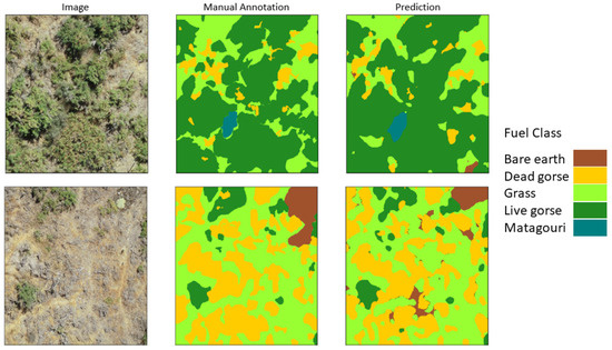
Figure 5.
Manual annotations vs. model predictions for two randomly selected images from the test set.

Figure 4.
Percentage-wise confusion matrix showing per class accuracy (equivalent to recall along the diagonals) and misclassification proportions (non-diagonals) for the various manual fuel type annotations compared with model predictions for the test dataset of 27,620,352 pixels (37 images).
Figure 4.
Percentage-wise confusion matrix showing per class accuracy (equivalent to recall along the diagonals) and misclassification proportions (non-diagonals) for the various manual fuel type annotations compared with model predictions for the test dataset of 27,620,352 pixels (37 images).

3.2. Accuracy of Biomass and Fuel Load Predictions from ULS and UAV Imagery
The correlation analysis between the destructive sampling and metrics derived from ULS (Table 3) and semantic segmentation (Table 4) demonstrated wide variation, with R2 ranging from 0 to 0.76 for TAGB (Figure 6a) and from 0 to 0.69 for AGAF (Figure 6b). The results for each metric were similar for AGAF and TAGB (Figure 6). The highest correlation for TAGB was observed with the structural metric ZPCUM9, with an R2 of 0.76 (Figure 7a). Other highly correlated metrics were all structural and included ZPCUM8, ZQ05 and ZQ10 with R2 of 0.72, 0.63 and 0.59, respectively (Figure 6a). The highest correlation observed for AGAF was with ZQ05, with an R2 of 0.69 (Figure 7c). As with TAGB, other highly correlated metrics were all structural and included ZPCUM8, ZQ10 and ZPCUM9 with R2 of 0.67, 0.63 and 0.59, respectively (Figure 6b).
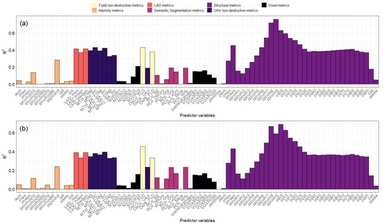
Figure 6.
Performance of the lidar and field-measured metrics in predicting (a) TAGB and (b) AGAF, coloured by the type of predictor variable.
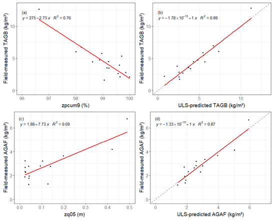
Figure 7.
Plots showing the correlation between (a) TAGB and ZPCUM9, (b) the relationship between actual biomass and predictions obtained from our best model with three variables (ZPCUM9, ZKURT and VOXPO05), (c) the correlation between AGAF and ZQ05, and (d) the relationship between actual fuel load and predictions obtained from our best model with three variables (ZQ05, NVOX02 and ZPCUM1). Solid red lines represent the line of best fit for the fitted linear models, and in (b,d), the dashed black line represents the 1:1 line.
For TAGB, a linear model with ZPCUM9 was developed (Figure 7a), and residuals from this model showed a wide range in correlation with the set of variables (R2 = 0 to 0.39). The strongest correlation that made sense was between ZKURT and TAGB with R2 = 0.34. Other notable correlations with fuel load included VOXPO20 and VOXPO10 with R2 of 0.28 and 0.24. The two-variable model for TAGB produced from ZPCUM9 and ZKURT showed a strong correlation with fuel load with an R2 = 0.85 and an RMSE of 1.01 kg/m2 (Table 6). For AGAF, a linear model with ZQ05 (Figure 7c) was developed, and residuals from this model showed a wide range in correlation with the set of variables (R2 = 0 to 0.37). The strongest correlation was between NVOX02 and AGAF, with R2 = 0.37. Other notable correlations with fuel load included ITOT and NVOX01, both with R2 of 0.37. The two-variable model for AGAF produced from ZQ05 and NVOX02 showed a strong correlation with fuel load, with an R2 = 0.81 and an RMSE of 0.56 kg/m2 (Table 6).
Table 6.
Statistics for the two multiple regression models. Shown are root mean square error (RMSE), relative RMSE (RMSE%), model cumulative coefficient of determination (R2) and partial R2 (i.e., gain in R2 resulting from inclusion of the variable). For the significance category, the t values and p categories from t-tests are shown, with asterisks ***, *, respectively, representing significance at p = 0.001 and 0.05. The variance inflation factor (VIF) is also shown.
Residuals from the two variable models were plotted against the variable set. Variation in the correlation between residuals and variables ranged from R2 = 0 to 0.28 for TAGB, with VOXPO05 showing the strongest correlation, and R2 = 0 to 0.37 for AGAF, with NVOX02 displaying the strongest correlation. The final models that included ZPCUM9, ZKURT and VOXPO05 for TAGB, and ZQ05, NVOX02 and ZPCUM1 for AGAF were more precise predictors than the second models with R2 values of = 0.89 and 0.87, respectively, and RMSE values of 0.84 kg/m2 (18.6%) and 0.51 kg/m2 (11.3%). A plot of predicted against actual values for these final models showed little apparent bias (Figure 7b,d). All variables in the model were significant, and the variance inflation factor was very low for all variables (Table 6). Figure 8 shows three plots across the range of the vegetation plots, showing (a) high, (b) medium and (c) low levels of TAGB, AGAF and overstory height (OsHt) along with the variation in independent variables.
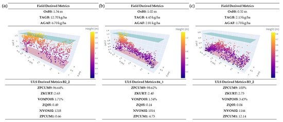
Figure 8.
Height normalised ULS point cloud plots representing the range in physical metrics within the vegetation plots and the corresponding ULS structural metrics, showing (a) high, (b) medium and (c) low levels of OsHt, TAGB and AGAF. Variation in the independent variables included in the model are shown below the figure. Red and Green surfaces, respectively, represent the first and ninth height deciles, up to which the cumulative percentage of points are calculated to derive ZPCUM1 and ZPCUM9.
3.3. Accuracy of Biomass and Fuel Load Predictions from Non-Destructive Field Methodology and UAV Equivalents
Model predictions of fuel load (AGAF) and biomass (TAGB) using field-measured OsHt, and predictions of TAGB using field-measured OsCo did not perform as well as the two models that used UAV-derived versions of these metrics. Predictions of AGAF using field-measured OsCo, however, performed better than the UAV-derived alternative. Correlations between TAGB and the field-measured variables were of weak to moderate strength, with R2 values of 0.38 and 0.11 for models that used field-measured overstory height (OsHt_FLD) and cover (OsCo_FLD), respectively (Figure 9a,b). Correlations between AGAF and the field-measured variables were of modest to moderate strength, with R2 values of 0.33 and 0.45 for models that used field-measured overstory height (OsHt_FLD) and cover (OsCo_FLD), respectively (Figure 9d,e). When a two variable model was created from OsHt_FLD and OsCo_FLD, as per [24], the model predicted TAGB and AGAF with correlations of R2 = 0.50 and 0.49, respectively, with RMSE values of 1.81 kg/m2 (40%) and 1.39 kg/m2 (30.8%), respectively (Figure 9c,f). When these same metrics were predicted from the UAV data, both MTH_PC (equivalent to OsHt_FLD) and OsCo showed stronger correlations with TAGB (R2 = 0.43 and 0.19, respectively) than field measured OsHt and OsCo (Figure 9g,h) and stronger correlations between UAV-measured MTH_PC and AGAF (R2 = 0.38; Figure 9j). When combined into a two variable model, the model predicted TAGB and AGAF with moderate correlations of R2 = 0.44 and 0.41, with RMSE values of 1.56 kg/m2 (34.5%) and 0.98 kg/m2 (21.7%), respectively (Figure 9i,l).
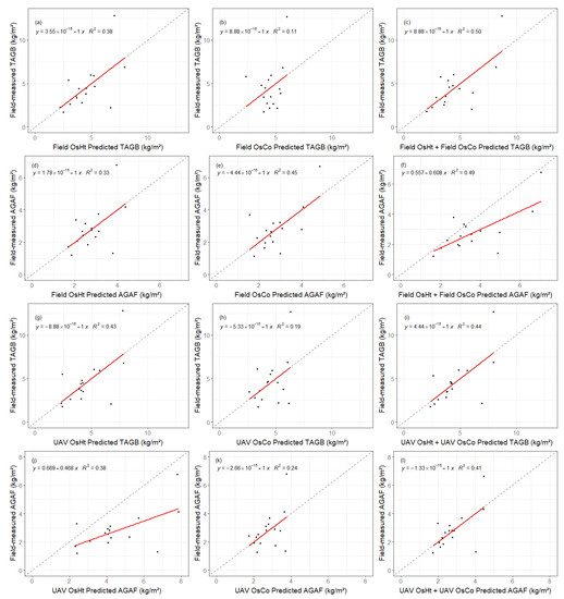
Figure 9.
Plots showing correlation between (a) destructively sampled TAGB and field-measured (a) OsHt, (b) OsHt, (c) OsHt + OsCo, (g) UAV-sampled OsHt, (h) UAV-measured OsCo and (i) UAV-sampled OsHt + OsCo; destructively sampled AGAF and field-measured (d) OsHt, (e) OsHt, (f) OsHt + OsCo, (j) UAV-sampled OsHt, (k) UAV-measured OsCo and (l) UAV-sampled OsHt + OsCo. The dashed black line represents the 1:1 line, and the solid red line and equation represents the line of best fit.
4. Discussion
4.1. Fuel Load and Biomass Predictions from ULS
This study showed that metrics derived from ULS data could be used to precisely predict biomass (TAGB) (R2 = 0.89) and fuel load (AGAF) (R2 = 0.87). Comparing this with the literature, this model has the highest precision among studies that have used ALS to predict biomass (R2 = 0.63–0.88) [23,32,33] and was stronger than a previous study for deriving shrub biomass from ALS (R2 = 0.76) [38]. These results are at the upper end of the correlation range for studies predicting shrub biomass using TLS (R2 = 0.71–0.94) [22,39,51,58,96] and were higher than a model from a previous study that derived understory shrub fuel load from TLS (R2 = 0.83) [45]. These findings support the assertion by [22] that ULS is an effective intermediate platform between ALS and TLS that combines the scaling available from aerial captures with the higher resolution vegetation description associated with methods such as TLS. In terms of accuracy, our models were able to predict TAGB and AGAF with high levels of accuracy (RMSE = 0.84 kg/m2/18.6% and RMSE = 0.51 kg/m2/11.3%, respectively). When compared with the literature, our model for TAGB fell within the lower end of accuracy values reported in the literature for ALS for predicting biomass (RMSE = 2.4 to 19.2%) [23,33,38]. Our results, however, showed a marked improvement on reported values of accuracy for predicting biomass with TLS (RMSE = 16.5–165.1%) [22,39,58].
Previous studies have shown that the analysis of lidar structural metrics from ALS data are very effective at predicting vegetation [23,32,33] and shrub biomass [38]. Although structural metrics from TLS data have been used to predict shrub biomass [22], volumetric or voxel metrics are more common predictors of shrub biomass [39,51,96] or fuel load [45] from TLS. In terms of correlation, the best results reported in the literature from TLS were derived from voxel metrics with R2 values of 0.90–0.94 ([39] and [51], respectively). The use of structural metrics has been reported to produce a weaker correlation of R2 = 0.71 [22]. Previous studies have noted that structural metrics from ALS have R2 ranging from 0.76 to 0.88 ([33] and [38], respectively). Our results show that structural metrics were more strongly related to TAGB than voxel metrics, with maximum R2 of 0.76 (ZPCUM9) and 0.34 (VOXPO20), respectively, for these two classes. This suggests that the structural metrics are a more effective tool for airborne data. One potential reason for this disparity could be due to beam divergence. A previous study noted that as the distance between the scanner and the target increases, the beam divergence (and therefore the laser footprint size) also increases, which reduces the likelihood of the laser penetrating through gaps in vegetation without triggering a return [59]. This in turn would result in less refined characterization of the lower strata of the shrub layers and the internal structure of denser shrub vegetation. ALS data are inherently captured at greater distances from the target than TLS. It therefore seems reasonable to assume that ALS point clouds would be less representative of the entire vegetation structure than TLS point clouds. Point density could also influence the accuracy of the vegetation characterisation. Even though the point density of the ULS in this study was very high for airborne data (306 ppm2), this is still vastly lower than the point densities reported by TLS studies, which largely use the Riegl VZ-1000 sensor [22,39,96]. This sensor can capture point clouds with densities of 1500–2500 ppm2 in shrub environments [97] with a nominal point spacing of 1 mm at a distance of 2 m [51], allowing for greater coverage of the overall vegetation structure. Future research should focus on capturing ULS data at different altitudes and comparing it with TLS data to see whether scanner distance and point density do influence the utility of voxel metrics. It should also be noted that, although lidar intensity metrics were assessed, the intensity values were not normalised. Future studies should see whether the normalisation of these values improves the ability of these metrics to predict fuel loadings or biomass.
Whilst these results are encouraging, the study was limited in the number of ground plots that were used for validation. Destructive sampling of plots is a laborious and costly task; however, future studies should look to use a larger data set with more plots across the range of biomass and potentially across multiple sites with different growing conditions, which would give a greater understanding of the ULS metrics and predictor variables that are underpinning the models. It would also be interesting for future studies to assess whether the same structural metrics that underpin the models in this study also perform well in similar or different vegetation types.
4.2. Fuel Load and Biomass Predictions from Non-Destructive Field Methodology and UAV Equivalents
An alternative to destructive sampling that has been employed prior to the advent of remote sensing is non-destructive sampling methods. A previous analysis by Pearce et al. [24] found high levels of precision in gorse between destructively sampled measurements of AGAF and field-measured OsHt (RMSE = 21.9%), for a combination of field-measured OsHt and OsCo (RMSE = 20.2%), and between destructively sampled TAGB and OsHt (RMSE = 19.2%). When we applied this methodology to the field measurements for OsHt and OsCo collected in this study, we found lower relative RMSEs of 40% for TAGB and 30.8% for AGAF, which are substantially poorer than the results reported in the original study. The results from the ULS structural metrics, however, provided a higher level of precision (18.6%; Table 6), which is a slight improvement on the non-destructive results from [24]. This suggests that our method can predict TAGB across an area with higher levels of precision than the field sampling method using less data points, as there were only 16 plots in this study compared with 55 in [24]. The gorse model in [24] was, however, developed from sites with relatively homogeneous shrub cover, so may not be that representative of this particular site where cover was more patchy. The model from [24] was also produced from sampling at multiple gorse sites across New Zealand, with different climates, soils, land management histories, and therefore growth rates and vegetation structures. It is likely that stronger relationships could have been developed for individual sites, depending on the number of samples at each site. Future research should use structural metrics derived from ULS data across a greater number of plots and from a range of sites to assess whether the accuracy of the model changes.
The cost of ULS is generally quite prohibitive, and although some sensors are now becoming more affordable, it has previously been noted that SfM could provide a lower cost alternative to ULS [57]. From our results, we were able to extract the same metrics (OsHt and OsCo) used to predict TAGB and AGAF in [24] from the UAV data and found that results were comparable for field-derived metrics of TAGB and AGAF (R2 = 0.50; RMSE = 40% and R2 = 0.49; RMSE = 30.8%, respectively) and UAV-derived metrics of TAGB and AGAF (R2 = 0.44; RMSE = 34.5% and R2 = 0.41; RMSE = 21.7%, respectively). Previous research has found that height information from SfM data is comparable in accuracy to ULS [60,98], and therefore, SfM could be a viable option for predicting TAGB or AGAF in shrublands and other vegetation types, using a remotely sensed version of the Pearce et al. [24] method.
4.3. Fuel Class Prediction from Semantic Segmentation
The results of the deep learning segmentation of the UAV imagery overall showed a high level of accuracy (0.83 precision, recall and F1) weighted across all classes, with a minimum per class F1 score of 0.70. Very few studies have applied semantic segmentation of imagery to the classification of fuel types or fuel components within a fuel type, particularly in the multi-class context. To our knowledge, this is the first published study that has attempted to classify multiple fuel categories from ultra-high resolution UAV imagery using semantic segmentation. Other studies have classified fuel types from terrestrial imagery [99,100]. Our results for overall accuracy per class are at the upper range of reported accuracies (0.44–0.99) when compared with other studies that have classified different vegetation classes using deep learning methods [72,73,101,102,103]. Another study that also used a ResNet-50 encoder but with a SegNet segmentation model classified four categories of wetland vegetation communities from 1.8 cm GSD UAV imagery and reported F1 scores ranging from 0.75 to 0.92 [71].
Of the fuel categories that were assessed in this study, live gorse returned the best results (IoU = 0.83, precision = 0.89, recall = 0.92). Live gorse was most often confused with grass (5%) and dead gorse (2%) (Figure 4). It is likely that live gorse was confused with dead gorse due to labelling errors or similarities in appearance. Grass also often bordered the live gorse on the site, and it is likely that this caused some digitisation errors.
Matagouri performance was good considering it was heavily underrepresented in the training dataset (Figure 3). This suggests that it often displays unique spectral characteristics. It was sometimes confused with gorse (14%) and grass (10%), but this can likely be improved by collecting more imagery containing matagouri.
There was a moderate correlation between the training dataset prevalence and the per class accuracy. Although Dice-Loss gives acceptable performance in the presence of class imbalance, future studies should consider testing other loss functions to better account for the imbalance, such as Unified Focal Loss [104]. Techniques such as oversampling may also improve performance.
Other sources of errors are likely due to similarities among pixel composition between classes and labelling errors. As an example, the boundary of bare earth and grass can be difficult to distinguish for a human. Similarly, light coloured dead grass can easily be confused with dead gorse when annotating so it is not surprising that it also confused by the neural network. Mislabelling of classes can confuse the model and have an insignificant impact on the quantitative and qualitative results. We estimate labelling errors to be at least 5% of all pixels and note that the model was able to perform better than our manual annotation method in some smaller regions where the wrong class had been assigned.
Overall, the high level of accuracy of the deep learning segmentation demonstrated the utility of this method for fuel type classification. It was assumed that higher resolution imagery would enable more accurate annotations; however, the additional detail can create difficult labelling decisions in smaller regions and slow down the labelling process when trying to assign pixels to a class. Future work could look at comparing different GSD imagery to see whether a model can be trained on this ultra-high resolution imagery and then scaled using lower resolutions. Additional studies should focus on whether there is a benefit to using higher resolution imagery or if lower resolutions will suffice, helping to keep data size and capture times more practical. These options would make this technology more deployable for large-scale areas or wildfires using data from airborne (manned) or even space-borne platforms.
5. Conclusions
The developed models of biomass/fuel load and fuel type categories had high precision and accuracy. A key finding of our study was that UAVs can be used to capture fuel load data over larger areas to a higher level of precision and accuracy than current non-destructive methodologies. This could help to reduce the cost and complexity of fuel sampling operations, especially as the costs associated with sensors and data processing decrease and would prove to be a highly complementary method to existing field-based techniques. These tools allow for rapid data capture and analysis, which are crucial factors when dealing with active fire situations. Additionally, these methods could be used to build libraries of fuel types for different regions as input to fuel classification models that could be accessed and used for fuel management and wildfire preparedness operations. In summary, UAVs provide a useful supplementary platform that enables the expansion of fuel modelling and characterisation. Despite the encouraging results, we were constrained by data and further research should verify the key findings of this study using data from a larger number of plots, sites and fuel types.
Author Contributions
Conceptualization, R.J.L.H., V.R.C. and H.G.P.; methodology, R.J.L.H., K.O.M., V.R.C., S.A.-A. and S.J.D.; formal analysis, R.J.L.H., S.J.D. and M.S.W.; investigation, R.J.L.H.; resources, R.J.L.H.; data curation, R.J.L.H., P.D.M., S.J.D., S.A.-A. and K.O.M.; writing—original draft preparation, R.J.L.H., M.S.W. and S.J.D.; writing—review and editing, H.G.P., M.S.W., K.O.M. and S.A.-A.; visualization, R.J.L.H. and S.J.D.; supervision, R.J.L.H.; project administration, R.J.L.H.; funding acquisition, H.G.P. and R.J.L.H. All authors have read and agreed to the published version of the manuscript.
Funding
This research was supported by the Ministry of Business, Innovation and Employment (MBIE), New Zealand, through two research programmes: grant number C04X1602 entitled “Preparing New Zealand for Extreme Fire” and grant number C04X2103 “Extreme wildfire: Our new reality—are we ready?”.
Data Availability Statement
The data presented in this study are available on reasonable request from the corresponding author.
Acknowledgments
The authors thank Grant D. Pearse of Scion for his advice regarding the deep learning methodology, as well as Dilshan de Silva and Honey Jane Estarija of Scion for assistance with the preparation of the deep learning dataset and the photogrammetry optimisation trial. We also acknowledge Amritagandha Dutta, Lakshay Mehra and Satya Prakash Dash of Expand AI for their services in creating the semantic segmentation annotations used to train our model. Thanks are also due to Hugh Wallace from Scion’s Fire and Atmospheric Sciences Team for organising the establishment of the burn blocks that we carried out our research in and Alan Leckie, Rory Clifford, David Glogoski and Max Novoselov from Scion, who assisted with the field sampling.
Conflicts of Interest
The authors declare no conflict of interest.
Appendix A. Ambient Study Site Conditions
Table A1.
Summary of recorded weather during sampling of vegetation. Data were recorded every minute, and values presented include minimum value (min), maximum value (max) and standard deviation (SD). Rain values of 0 are depicted as precipitation was absent during these dates.
Table A1.
Summary of recorded weather during sampling of vegetation. Data were recorded every minute, and values presented include minimum value (min), maximum value (max) and standard deviation (SD). Rain values of 0 are depicted as precipitation was absent during these dates.
| Date | Temperature (°C) | Relative Humidity (%) | Wind Speed (m/s) | Rain | |||||||||
|---|---|---|---|---|---|---|---|---|---|---|---|---|---|
| Min. | Max. | Mean | SD | Min. | Max. | Mean | SD | Min. | Max. | Mean | SD | ||
| 6 February 2020 | 10.2 | 22.8 | 14.9 | 3.3 | 35.4 | 92.5 | 64.5 | 17.2 | 1.4 | 11.3 | 7.3 | 1.6 | 0 |
| 7 February 2020 | 6.4 | 23.5 | 15.2 | 4.8 | 32.0 | 95.9 | 64.8 | 21.1 | 0.3 | 11.1 | 3.9 | 2.6 | 0 |
| 8 February 2020 | 7.4 | 18.1 | 12.5 | 2.5 | 34.6 | 86.8 | 64.9 | 16.7 | 0.4 | 13.6 | 6.2 | 2.9 | 0 |
| 9 February 2020 | 2.8 | 23.4 | 13.6 | 6.3 | 33.9 | 97.3 | 64.5 | 22.2 | 0.2 | 9.2 | 3.6 | 1.9 | 0 |
| 10 February 2020 | 5.7 | 27.6 | 16.6 | 6.8 | 25.7 | 97.0 | 65.3 | 23.4 | 0.2 | 11.2 | 3.8 | 2.6 | 0 |
| 11 February 2020 | 7.8 | 26.3 | 16.7 | 5.5 | 29.7 | 95.5 | 72.0 | 18.2 | 0.2 | 11.3 | 4.2 | 3.3 | 0 |
| 12 February 2020 | 9.5 | 31.6 | 20.2 | 7.5 | 15.7 | 96.8 | 55.7 | 33.7 | 0.2 | 11.0 | 5.2 | 2.5 | 0 |
| 13 February 2020 | 11.5 | 27.6 | 17.6 | 4.7 | 27.9 | 95.9 | 71.8 | 19.3 | 0.0 | 14.0 | 5.2 | 3.4 | 0 |
| 14 February 2020 | 10.8 | 17.7 | 13.6 | 2.1 | 66.0 | 95.7 | 83.3 | 8.8 | 0.5 | 10.1 | 5.3 | 2.0 | 0 |
| 15 February 2020 | 12.2 | 27.0 | 18.0 | 4.7 | 20.0 | 90.9 | 64.8 | 22.1 | 0.0 | 13.8 | 5.2 | 3.6 | 0 |
| 16 February 2020 | 19.2 | 24.7 | 21.9 | 1.2 | 36.1 | 65.4 | 53.2 | 7.8 | 5.2 | 18.8 | 11.9 | 2.7 | 0 |
| 17 February 2020 | 20.5 | 29.4 | 23.8 | 2.5 | 39.1 | 73.4 | 58.8 | 9.8 | 3.9 | 17.6 | 8.9 | 2.9 | 0 |
| 18 February 2020 | 15.1 | 28.7 | 22.4 | 3.8 | 32.7 | 86.4 | 56.5 | 15.7 | 0.1 | 12.8 | 6.6 | 3.0 | 0 |
| 19 February 2020 | 12.4 | 26.4 | 19.4 | 3.5 | 33.3 | 81.8 | 57.3 | 11.6 | 0.3 | 12.4 | 7.1 | 2.6 | 0 |
| 20 February 2020 | 7.8 | 22.5 | 16.6 | 4.8 | 25.6 | 96.2 | 66.0 | 21.2 | 0.2 | 11.2 | 3.5 | 2.6 | 0 |
References
- Schulze, S.S.; Fischer, E.C.; Hamideh, S.; Mahmoud, H. Wildfire impacts on schools and hospitals following the 2018 California Camp Fire. Nat. Hazards 2020, 104, 901–925. [Google Scholar] [CrossRef]
- Boer, M.M.; de Dios, V.R.; Bradstock, R.A. Unprecedented burn area of Australian mega forest fires. Nat. Clim. Chang. 2020, 10, 171–172. [Google Scholar] [CrossRef]
- Shi, G.; Yan, H.; Zhang, W.; Dodson, J.; Heijnis, H.; Burrows, M. Rapid warming has resulted in more wildfires in northeastern Australia. Sci. Total Environ. 2021, 771, 144888. [Google Scholar] [CrossRef]
- Benali, A.; Sá, A.C.; Pinho, J.; Fernandes, P.M.; Pereira, J. Understanding the impact of different landscape-level fuel management strategies on wildfire hazard in central Portugal. Forests 2021, 12, 522. [Google Scholar] [CrossRef]
- Gaur, A.; Bénichou, N.; Armstrong, M.; Hill, F. Potential future changes in wildfire weather and behavior around 11 Canadian cities. Urban Clim. 2021, 35, 100735. [Google Scholar] [CrossRef]
- Huggins, T.J.; Langer, E.; McLennan, J.; Johnston, D.M.; Yang, L. The many-headed beast of wildfire risks in Aotearoa-New Zealand. Aust. J. Emerg. Manag. 2020, 35, 48–53. [Google Scholar]
- Pearce, H.G. The 2017 Port Hills wildfires—A window into New Zealand’s fire future. Aust. J. Disaster Trauma Stud. 2018, 22, 63–73. [Google Scholar]
- Christensen, B.; Herries, D.; Hartley, R.J.; Parker, R. UAS and smartphone integration at wildfire management in Aotearoa New Zealand. N. Z. J. For. Sci. 2021, 51, 10. [Google Scholar] [CrossRef]
- Langer, E.; Pearce, H.G.; Wegner, S. The urban side of the wildland-urban interface: A new fire audience identified following an extreme wildfire event in Aotearoa/New Zealand. In Proceedings of the Advances in Forest Fire Research 2018, Coimbra, Portugal, 10–16 November 2018; pp. 859–869. [Google Scholar]
- Anderson, W.R.; Cruz, M.G.; Fernandes, P.M.; McCaw, L.; Vega, J.A.; Bradstock, R.A.; Fogarty, L.; Gould, J.; McCarthy, G.; Marsden-Smedley, J.B. A generic, empirical-based model for predicting rate of fire spread in shrublands. Int. J. Wildland Fire 2015, 24, 443–460. [Google Scholar] [CrossRef]
- Grant, M.A.; Duff, T.J.; Penman, T.D.; Pickering, B.J.; Cawson, J.G. Mechanical mastication reduces fuel structure and modelled fire behaviour in Australian shrub encroached ecosystems. Forests 2021, 12, 812. [Google Scholar] [CrossRef]
- Alonzo, M.; Dial, R.J.; Schulz, B.K.; Andersen, H.E.; Lewis-Clark, E.; Cook, B.D.; Morton, D.C. Mapping tall shrub biomass in Alaska at landscape scale using structure-from-motion photogrammetry and lidar. Remote Sens. Environ. 2020, 245, 111841. [Google Scholar] [CrossRef]
- Kitzberger, T.; Perry, G.; Paritsis, J.; Gowda, J.; Tepley, A.; Holz, A.; Veblen, T. Fire–vegetation feedbacks and alternative states: Common mechanisms of temperate forest vulnerability to fire in southern South America and New Zealand. N. Z. J. Bot. 2016, 54, 247–272. [Google Scholar] [CrossRef]
- Baeza, M.; De Luıs, M.; Raventós, J.; Escarré, A. Factors influencing fire behaviour in shrublands of different stand ages and the implications for using prescribed burning to reduce wildfire risk. J. Environ. Manag. 2002, 65, 199–208. [Google Scholar] [CrossRef] [PubMed]
- Costello, D.A.; Lunt, I.D.; Williams, J.E. Effects of invasion by the indigenous shrub Acacia sophorae on plant composition of coastal grasslands in south-eastern Australia. Biolo. Conserv. 2000, 96, 113–121. [Google Scholar] [CrossRef]
- Mariani, M.; Connor, S.E.; Theuerkauf, M.; Herbert, A.; Kuneš, P.; Bowman, D.; Fletcher, M.S.; Head, L.; Kershaw, A.P.; Haberle, S.G. Disruption of cultural burning promotes shrub encroachment and unprecedented wildfires. Front. Ecol. Environ. 2022, 20, 292–300. [Google Scholar] [CrossRef]
- Krisanski, S.; Taskhiri, M.S.; Gonzalez Aracil, S.; Herries, D.; Muneri, A.; Gurung, M.B.; Montgomery, J.; Turner, P. Forest Structural Complexity Tool—An open source, fully-automated tool for measuring forest point clouds. Remote Sens. 2021, 13, 4677. [Google Scholar] [CrossRef]
- Masek, J.G.; Hayes, D.J.; Joseph Hughes, M.; Healey, S.P.; Turner, D.P. The role of remote sensing in process-scaling studies of managed forest ecosystems. For. Ecol. Manag. 2015, 355, 109–123. [Google Scholar] [CrossRef]
- Arroyo, L.A.; Pascual, C.; Manzanera, J.A. Fire models and methods to map fuel types: The role of remote sensing. For. Ecol. Manag. 2008, 256, 1239–1252. [Google Scholar] [CrossRef]
- Adhikari, B.; Xu, C.; Hodza, P.; Minckley, T. Developing a geospatial data-driven solution for rapid natural wildfire risk assessment. Appl. Geogr. 2021, 126, 102382. [Google Scholar] [CrossRef]
- Scott, J.H.; Thompson, M.P.; Calkin, D.E. A Wildfire Risk Assessment Framework for Land and Resource Management; Rocky Mountain Research Station: Fort Collins, CO, USA, 2013; p. 83. [Google Scholar]
- Anderson, K.E.; Glenn, N.F.; Spaete, L.P.; Shinneman, D.J.; Pilliod, D.S.; Arkle, R.S.; McIlroy, S.K.; Derryberry, D.R. Estimating vegetation biomass and cover across large plots in shrub and grass dominated drylands using terrestrial lidar and machine learning. Ecol. Indic. 2018, 84, 793–802. [Google Scholar] [CrossRef]
- Domingo, D.; Lamelas, M.T.; Montealegre, A.L.; García-Martín, A.; de la Riva, J. Estimation of total biomass in Aleppo pine forest stands applying parametric and nonparametric methods to low-density airborne laser scanning data. Forests 2018, 9, 158. [Google Scholar] [CrossRef]
- Pearce, H.; Anderson, W.; Fogarty, L.; Todoroki, C.; Anderson, S. Linear mixed-effects models for estimating biomass and fuel loads in shrublands. Can. J. For. Res. 2010, 40, 2015–2026. [Google Scholar] [CrossRef]
- Gale, M.G.; Cary, G.J.; Van Dijk, A.I.; Yebra, M. Forest fire fuel through the lens of remote sensing: Review of approaches, challenges and future directions in the remote sensing of biotic determinants of fire behaviour. Remote Sens. Environ. 2021, 255, 112282. [Google Scholar] [CrossRef]
- Kumar, L.; Mutanga, O. Remote Sensing of Above-Ground Biomass; Multidisciplinary Digital Publishing Institute: Basel, Switzerland, 2017. [Google Scholar]
- Leonardo, E.M.C.; Watt, M.S.; Pearse, G.D.; Dash, J.P.; Persson, H.J. Comparison of TanDEM-X InSAR data and high-density ALS for the prediction of forest inventory attributes in plantation forests with steep terrain. Remote Sens. Environ. 2020, 246, 111833. [Google Scholar] [CrossRef]
- Bright, B.C.; Hudak, A.T.; Meddens, A.J.H.; Hawbaker, T.J.; Briggs, J.S.; Kennedy, R.E. Prediction of forest canopy and surface fuels from lidar and satellite time series data in a bark beetle-affected forest. Forests 2017, 8, 322. [Google Scholar] [CrossRef]
- Domingo, D.; de la Riva, J.; Lamelas, M.T.; García-Martín, A.; Ibarra, P.; Echeverría, M.; Hoffrén, R. Fuel type classification using airborne laser scanning and Sentinel 2 data in Mediterranean forest affected by wildfires. Remote Sens. 2020, 12, 3660. [Google Scholar] [CrossRef]
- Kellner, J.R.; Armston, J.; Birrer, M.; Cushman, K.; Duncanson, L.; Eck, C.; Falleger, C.; Imbach, B.; Král, K.; Krůček, M. New opportunities for forest remote sensing through ultra-high-density drone lidar. Surv. Geophys. 2019, 40, 959–977. [Google Scholar] [CrossRef] [PubMed]
- Inan, M.; Bilici, E.; Akay, A.E. Using airborne lidar data for assessment of forest fire fuel load potential. In Proceedings of the ISPRS Annals of the Photogrammetry, Remote Sensing and Spatial Information Sciences, Kyiv, Ukraine, 4–6 December 2017; pp. 255–258. [Google Scholar]
- Chen, Y.; Zhu, X.; Yebra, M.; Harris, S.; Tapper, N. Estimation of forest surface fuel load using airborne LiDAR data. In Proceedings of the SPIE—The International Society for Optical Engineering, San Diego, CA, USA, 28 August–1 September 2016. [Google Scholar]
- Erdody, T.L.; Moskal, L.M. Fusion of LiDAR and imagery for estimating forest canopy fuels. Remote Sens. Environ. 2010, 114, 725–737. [Google Scholar] [CrossRef]
- Gajardo, J.; García, M.; Riaño, D. Applications of Airborne Laser Scanning in Forest Fuel Assessment and Fire Prevention. In Forestry Applications of Airborne Laser Scanning: Concepts and Case Studies; Maltamo, M., Næsset, E., Vauhkonen, J., Eds.; Springer: Dordrecht, The Netherlands, 2014; pp. 439–462. [Google Scholar] [CrossRef]
- García, M.; Saatchi, S.; Casas, A.; Koltunov, A.; Ustin, S.L.; Ramirez, C.; Balzter, H. Extrapolating forest canopy fuel properties in the California Rim fire by combining airborne LiDAR and landsat OLI data. Remote Sens. 2017, 9, 394. [Google Scholar] [CrossRef]
- Rodríguez-Puerta, F.; Ponce, R.A.; Pérez-Rodríguez, F.; Águeda, B.; Martín-García, S.; Martínez-Rodrigo, R.; Lizarralde, I. Comparison of machine learning algorithms for wildland-urban interface fuelbreak planning integrating als and uav-borne lidar data and multispectral images. Drones 2020, 4, 21. [Google Scholar] [CrossRef]
- Yebra, M.; Marselis, S.; Van Dijk, A.; Cary, G.; Chen, Y. Using LiDAR for Forest and Fuel Structure Mapping: Options, Benefits, Requirements and Costs; Bushfire & Natural Hazards CRC: East Melbourne, Australia, 2015. [Google Scholar]
- Li, A.; Dhakal, S.; Glenn, N.F.; Spaete, L.P.; Shinneman, D.J.; Pilliod, D.S.; Arkle, R.S.; McIlroy, S.K. Lidar aboveground vegetation biomass estimates in shrublands: Prediction, uncertainties and application to coarser scales. Remote Sens. 2017, 9, 903. [Google Scholar] [CrossRef]
- Li, A.; Glenn, N.F.; Olsoy, P.J.; Mitchell, J.J.; Shrestha, R. Aboveground biomass estimates of sagebrush using terrestrial and airborne LiDAR data in a dryland ecosystem. Agric. For. Meteorol. 2015, 213, 138–147. [Google Scholar] [CrossRef]
- Mitchell, J.J.; Glenn, N.F.; Sankey, T.T.; Derryberry, D.R.; Anderson, M.O.; Hruska, R.C. Small-footprint LiDAR estimations of sagebrush canopy characteristics. Photogramm. Eng. Remote Sens. 2011, 77, 521–530. [Google Scholar] [CrossRef]
- Swetnam, T.L.; Gillan, J.K.; Sankey, T.T.; McClaran, M.P.; Nichols, M.H.; Heilman, P.; McVay, J. Considerations for achieving cross-platform point cloud data fusion across different dryland ecosystem structural states. Front. Plant Sci. 2018, 8, 2144. [Google Scholar] [CrossRef] [PubMed]
- Wieser, M.; Hollaus, M.; Mandlburger, G.; Glira, P.; Pfeifer, N. ULS LiDAR supported analyses of laser beam penetration from different ALS systems into vegetation. In Proceedings of the ISPRS Annals of the Photogrammetry, Remote Sensing and Spatial Information Sciences, Prague, Czech Republic, 12–19 July 2016; pp. 233–239. [Google Scholar]
- Jakubowksi, M.K.; Guo, Q.; Collins, B.; Stephens, S.; Kelly, M. Predicting surface fuel models and fuel metrics using lidar and CIR imagery in a dense, mountainous forest. Photogramm. Eng. Remote Sens. 2013, 79, 37–49. [Google Scholar] [CrossRef]
- Estornell, J.; Ruiz, L.; Velázquez-Martí, B.; Hermosilla, T. Analysis of the factors affecting LiDAR DTM accuracy in a steep shrub area. Int. J. Digital Earth 2011, 4, 521–538. [Google Scholar] [CrossRef]
- Loudermilk, E.L.; Hiers, J.K.; O’Brien, J.J.; Mitchell, R.J.; Singhania, A.; Fernandez, J.C.; Cropper, W.P.; Slatton, K.C. Ground-based LIDAR: A novel approach to quantify fine-scale fuelbed characteristics. Int. J. Wildland Fire 2009, 18, 676–685. [Google Scholar] [CrossRef]
- Zhao, Y.; Liu, X.; Wang, Y.; Zheng, Z.; Zheng, S.; Zhao, D.; Bai, Y. UAV-based individual shrub aboveground biomass estimation calibrated against terrestrial LiDAR in a shrub-encroached grassland. Int. J. Appl. Earth Obs. Geoinf. 2021, 101, 102358. [Google Scholar] [CrossRef]
- Telling, J.; Lyda, A.; Hartzell, P.; Glennie, C. Review of Earth science research using terrestrial laser scanning. Earth-Sci. Rev. 2017, 169, 35–68. [Google Scholar] [CrossRef]
- Liu, G.; Wang, J.; Dong, P.; Chen, Y.; Liu, Z. Estimating individual tree height and diameter at breast height (DBH) from terrestrial laser scanning (TLS) data at plot level. Forests 2018, 8, 398. [Google Scholar] [CrossRef]
- Hackenberg, J.; Wassenberg, M.; Spiecker, H.; Sun, D. Non destructive method for biomass prediction combining TLS derived tree volume and wood density. Forests 2015, 6, 1274–1300. [Google Scholar] [CrossRef]
- Liang, X.; Hyyppä, J.; Kaartinen, H.; Lehtomäki, M.; Pyörälä, J.; Pfeifer, N.; Holopainen, M.; Brolly, G.; Francesco, P.; Hackenberg, J.; et al. International benchmarking of terrestrial laser scanning approaches for forest inventories. ISPRS J. Photogramm. Remote Sens. 2018, 144, 137–179. [Google Scholar] [CrossRef]
- Greaves, H.E.; Vierling, L.A.; Eitel, J.U.H.; Boelman, N.T.; Magney, T.S.; Prager, C.M.; Griffin, K.L. Estimating aboveground biomass and leaf area of low-stature Arctic shrubs with terrestrial LiDAR. Remote Sens. Environ. 2015, 164, 26–35. [Google Scholar] [CrossRef]
- Olsoy, P.J.; Glenn, N.F.; Clark, P.E. Estimating sagebrush biomass using terrestrial laser scanning. Rangel. Ecol. Manag. 2014, 67, 224–228. [Google Scholar] [CrossRef]
- Chen, Y.; Zhu, X.; Yebra, M.; Harris, S.; Tapper, N. Strata-based forest fuel classification for wild fire hazard assessment using terrestrial LiDAR. J. Appl. Remote Sens. 2016, 10, 046025. [Google Scholar] [CrossRef]
- Hiers, J.K.; O’Brien, J.J.; Mitchell, R.; Grego, J.M.; Loudermilk, E.L. The wildland fuel cell concept: An approach to characterize fine-scale variation in fuels and fire in frequently burned longleaf pine forests. Int. J. Wildland Fire 2009, 18, 315–325. [Google Scholar] [CrossRef]
- Wallace, L.; Gupta, V.; Reinke, K.; Jones, S. An assessment of pre- and post fire near surface fuel hazard in an australian dry sclerophyll forest using point cloud data captured using a Terrestrial Laser Scanner. Remote Sens. 2016, 8, 679. [Google Scholar] [CrossRef]
- Adams, T. Using Terrestrial LiDAR to Model Shrubs for Fire Behavior Simulation. Master’s Thesis, The University of Montana, Missoula, MT, USA, 2014. Available online: https://scholarworks.umt.edu/etd/4173 (accessed on 2 March 2022).
- Hudak, A.T.; Kato, A.; Bright, B.C.; Loudermilk, E.L.; Hawley, C.; Restaino, J.C.; Ottmar, R.D.; Prata, G.A.; Cabo, C.; Prichard, S.J.; et al. Towards spatially explicit quantification of pre- and postfire fuels and fuel consumption from traditional and point cloud measurements. For. Sci. 2020, 66, 428–442. [Google Scholar] [CrossRef]
- Rowell, E.; Loudermilk, E.L.; Hawley, C.; Pokswinski, S.; Seielstad, C.; Queen, L.L.; O’Brien, J.J.; Hudak, A.T.; Goodrick, S.; Hiers, J.K. Coupling terrestrial laser scanning with 3D fuel biomass sampling for advancing wildland fuels characterization. For. Ecol. Manag. 2020, 462, 117945. [Google Scholar] [CrossRef]
- Rowell, E.M.; Seielstad, C.A.; Ottmar, R.D. Development and validation of fuel height models for terrestrial lidar—RxCADRE 2012. Int. J. Wildland Fire 2016, 25, 38–47. [Google Scholar] [CrossRef]
- Hartley, R.J.; Leonardo, E.M.; Massam, P.; Watt, M.S.; Estarija, H.J.; Wright, L.; Melia, N.; Pearse, G.D. An assessment of high-density UAV point clouds for the measurement of young forestry trials. Remote Sens. 2020, 12, 4039. [Google Scholar] [CrossRef]
- Brede, B.; Lau, A.; Bartholomeus, H.M.; Kooistra, L. Comparing RIEGL RiCOPTER UAV LiDAR derived canopy height and DBH with terrestrial LiDAR. Sensors 2017, 17, 2371. [Google Scholar] [CrossRef] [PubMed]
- Madsen, B.; Treier, U.A.; Zlinszky, A.; Lucieer, A.; Normand, S. Detecting shrub encroachment in seminatural grasslands using UAS LiDAR. Ecol. Evol. 2020, 10, 4876–4902. [Google Scholar] [CrossRef] [PubMed]
- Fernández-álvarez, M.; Armesto, J.; Picos, J. LiDAR-based wildfire prevention in WUI: The automatic detection, measurement and evaluation of forest fuels. Forests 2019, 10, 148. [Google Scholar] [CrossRef]
- Chuvieco, E.; Riaño, D.; Van Wagtendok, J.; Morsdof, F. Fuel loads and fuel type mapping. In Wildland Fire Danger Estimation and Mapping: The Role of Remote Sensing Data; World Scientific: Singapore, 2003; pp. 119–142. [Google Scholar]
- Riaño, D.; Chuvieco, E.; Ustin, S.L.; Salas, J.; Rodríguez-Pérez, J.R.; Ribeiro, L.M.; Viegas, D.X.; Moreno, J.M.; Fernández, H. Estimation of shrub height for fuel-type mapping combining airborne LiDAR and simultaneous color infrared ortho imaging. Int. J. Wildland Fire 2007, 16, 341–348. [Google Scholar] [CrossRef]
- García, M.; Riaño, D.; Chuvieco, E.; Salas, J.; Danson, F.M. Multispectral and LiDAR data fusion for fuel type mapping using Support Vector Machine and decision rules. Remote Sens. Environ. 2011, 115, 1369–1379. [Google Scholar] [CrossRef]
- Gibril, M.B.A.; Shafri, H.Z.M.; Shanableh, A.; Al-Ruzouq, R.; Wayayok, A.; Hashim, S.J. Deep convolutional neural network for large-scale date palm tree mapping from UAV-based images. Remote Sensing 2021, 13, 2787. [Google Scholar] [CrossRef]
- Bah, M.D.; Dericquebourg, E.; Hafiane, A.; Canals, R. Deep learning based classification system for identifying weeds using high-resolution UAV imagery. In Proceedings of the Science and Information Conference, London, UK, 10–12 July 2018; pp. 176–187. [Google Scholar]
- Huang, H.; Deng, J.; Lan, Y.; Yang, A.; Deng, X.; Zhang, L. A fully convolutional network for weed mapping of unmanned aerial vehicle (UAV) imagery. PLoS ONE 2018, 13, e0196302. [Google Scholar] [CrossRef]
- Pearse, G.D.; Tan, A.Y.; Watt, M.S.; Franz, M.O.; Dash, J.P. Detecting and mapping tree seedlings in UAV imagery using convolutional neural networks and field-verified data. ISPRS J. Photogramm. Remote Sens. 2020, 168, 156–169. [Google Scholar] [CrossRef]
- Bhatnagar, S.; Gill, L.; Ghosh, B. Drone image segmentation using machine and deep learning for mapping raised bog vegetation communities. Remote Sens. 2020, 12, 2602. [Google Scholar] [CrossRef]
- Kattenborn, T.; Eichel, J.; Fassnacht, F.E. Convolutional Neural Networks enable efficient, accurate and fine-grained segmentation of plant species and communities from high-resolution UAV imagery. Sci. Rep. 2019, 9, 1–9. [Google Scholar] [CrossRef] [PubMed]
- Trenčanová, B.; Proença, V.; Bernardino, A. Development of semantic maps of vegetation cover from UAV images to support planning and management in fine-grained fire-prone landscapes. Remote Sens. 2022, 14, 1262. [Google Scholar] [CrossRef]
- Finney, M.A.; Pearce, H.G.; Strand, T.; Katurji, M.; Clements, C. New Zealand prescribed fire experiments to test convective heat transfer in wildland fires. In Proceedings of the Advances in Forest Fire Research 2018, Coimbra, Portugal, 11–18 November 2018; pp. 1288–1292. [Google Scholar]
- Pearce, H.G.; Finney, M.A.; Strand, T.; Katurji, M.; Clements, C. New Zealand field-scale fire experiments to test convective heat transfer in wildland fires. In Proceedings of the 6th International Fire Behavior and Fuels Conference, Sydney, Australia, 29 April–3 May 2019. [Google Scholar]
- Meroney, R.N. Wind-tunnel simulation of the flow over hills and complex terrain. J. Wind Eng. Ind. Aerodyn. 1980, 5, 297–321. [Google Scholar] [CrossRef]
- McRae, D.J.; Alexander, M.E.; Stocks, B.J. Measurement and Description of Fuels and Fire Behaviour on Prescribed Burns: A Handbook; Department of the Environment, Canadian Forest Service, Great Lakes Forest Research Centre: Sault Ste. Marie, ON, Canada, 1979; Volume Rep. O-X-287.
- Tonkin, T.N.; Midgley, N.G. Ground-control networks for image based surface reconstruction: An investigation of optimum survey designs using UAV derived imagery and structure-from-motion photogrammetry. Remote Sens. 2016, 8, 786. [Google Scholar] [CrossRef]
- Gindraux, S.; Boesch, R.; Farinotti, D. Accuracy assessment of digital surface models from unmanned aerial vehicles’ imagery on glaciers. Remote Sens. 2017, 9, 186. [Google Scholar] [CrossRef]
- Dandois, J.P.; Olano, M.; Ellis, E.C. Optimal altitude, overlap, and weather conditions for computer vision uav estimates of forest structure. Remote Sens. 2015, 7, 13895–13920. [Google Scholar] [CrossRef]
- Roth, L.; Hund, A.; Aasen, H. PhenoFly Planning Tool: Flight planning for high-resolution optical remote sensing with unmanned areal systems. Plant Methods 2018, 14, 1–21. [Google Scholar] [CrossRef]
- O’Connor, J.; Smith, M.J.; James, M.R. Cameras and settings for aerial surveys in the geosciences: Optimising image data. Prog. Phys. Geogr. 2017, 41, 325–344. [Google Scholar] [CrossRef]
- Frey, J.; Kovach, K.; Stemmler, S.; Koch, B. UAV photogrammetry of forests as a vulnerable process. A sensitivity analysis for a structure from motion RGB-image pipeline. Remote Sens. 2018, 10, 912. [Google Scholar] [CrossRef]
- Riegl. RIEGL miniVUX-1UAV Datasheet. Available online: https://www.riegl.com/uploads/tx_pxpriegldownloads/RIEGL_miniVUX-1UAV_Datasheet_2021-09-14.pdf (accessed on 2 June 2020).
- Isenburg, M. LAStools—Efficient LiDAR Processing Software, 190404; LAStools: Gilching, Germany, 2019. [Google Scholar]
- R Core Team. R: A Language and Environment for Statistical Computing; R Foundation for Statistical Computing: Vienna, Austria, 2020. [Google Scholar]
- Roussel, J.-R.; Auty, D.; De Boissieu, F.; Meador, A. lidR: Airborne LiDAR Data Manipulation and Visualization for Forestry Applications. R Package Version 2018, 1. Available online: https://github.com/Jean-Romain/lidR (accessed on 2 March 2021).
- Almeida, D.R.A.d.; Stark, S.C.; Shao, G.; Schietti, J.; Nelson, B.W.; Silva, C.A.; Gorgens, E.B.; Valbuena, R.; Papa, D.d.A.; Brancalion, P.H.S. Optimizing the remote detection of tropical rainforest structure with airborne lidar: Leaf area profile sensitivity to pulse density and spatial sampling. Remote Sens. 2019, 11, 92. [Google Scholar] [CrossRef]
- Woods, M.; Lim, K.; Treitz, P. Predicting forest stand variables from LIDAR data in the Great Lakes St. Lawrence Forest of Ontario. For. Chronicle 2008, 84, 827–839. [Google Scholar] [CrossRef]
- Chen, L.-C.; Zhu, Y.; Papandreou, G.; Schroff, F.; Adam, H. Encoder-decoder with atrous separable convolution for semantic image segmentation. In Proceedings of the European Conference on Computer Vision (ECCV), Munich, Germany, 8–14 September 2018; pp. 801–818. [Google Scholar]
- He, K.; Zhang, X.; Ren, S.; Sun, J. Deep residual learning for image recognition. In Proceedings of the 2016 IEEE Conference on Computer Vision and Pattern Recognition, Las Vegas, NV, USA, 27–30 June 2016; pp. 770–778. [Google Scholar]
- Deng, J.; Dong, W.; Socher, R.; Li, L.-J.; Li, K.; Fei-Fei, L. Imagenet: A large-scale hierarchical image database. In Proceedings of the 2009 IEEE Conference on Computer Vision and Pattern Recognition, Miami, FL, USA, 20–25 June 2009; pp. 248–255. [Google Scholar]
- Yakubovskiy, P. Segmentation Models Pytorch; GitHub Repository: San Francisco, CA, USA, 2020. [Google Scholar]
- Paszke, A.; Gross, S.; Massa, F.; Lerer, A.; Bradbury, J.; Chanan, G.; Killeen, T.; Lin, Z.; Gimelshein, N.; Antiga, L. Pytorch: An imperative style, high-performance deep learning library. In Proceedings of the Advances in Neural Information Processing Systems, Vancouver, BC, Canada, 8–14 December 2019; pp. 8024–8035. [Google Scholar]
- Pedregosa, F.; Varoquaux, G.; Gramfort, A.; Michel, V.; Thirion, B.; Grisel, O.; Blondel, M.; Prettenhofer, P.; Weiss, R.; Dubourg, V. Scikit-learn: Machine learning in Python. J. Mach. Learn. Res. 2011, 12, 2825–2830. [Google Scholar]
- Olsoy, P.J.; Glenn, N.F.; Clark, P.E.; Derryberry, D.R. Aboveground total and green biomass of dryland shrub derived from terrestrial laser scanning. ISPRS J. Photogramm. Remote Sens. 2014, 88, 166–173. [Google Scholar] [CrossRef]
- Sankey, T.; Donager, J.; McVay, J.; Sankey, J.B. UAV lidar and hyperspectral fusion for forest monitoring in the southwestern USA. Remote Sens. Environ. 2017, 195, 30–43. [Google Scholar] [CrossRef]
- Wallace, L.; Lucieer, A.; Malenovskỳ, Z.; Turner, D.; Vopěnka, P. Assessment of forest structure using two UAV techniques: A comparison of airborne laser scanning and structure from motion (SfM) point clouds. Forests 2016, 7, 62. [Google Scholar] [CrossRef]
- Cameron, H.A.; Panda, P.; Barczyk, M.; Beverly, J.L. Estimating boreal forest ground cover vegetation composition from nadir photographs using deep convolutional neural networks. Ecol. Inform. 2022, 69, 101658. [Google Scholar] [CrossRef]
- Labenski, P.; Ewald, M.; Schmidtlein, S.; Fassnacht, F.E. Classifying surface fuel types based on forest stand photographs and satellite time series using deep learning. Int. J. Appl. Earth Obs. Geoinf. 2022, 109, 102799. [Google Scholar] [CrossRef]
- Ayhan, B.; Kwan, C. Tree, shrub, and grass classification using only RGB images. Remote Sens. 2020, 12, 1333. [Google Scholar] [CrossRef]
- Sandino, J.; Gonzalez, F.; Mengersen, K.; Gaston, K.J. UAVs and machine learning revolutionising invasive grass and vegetation surveys in remote arid lands. Sensors 2018, 18, 605. [Google Scholar] [CrossRef]
- Wang, L.; Zhou, Y.; Hu, Q.; Tang, Z.; Ge, Y.; Smith, A.; Awada, T.; Shi, Y. Early detection of encroaching woody Juniperus virginiana and its classification in multi-species forest using UAS imagery and semantic segmentation algorithms. Remote Sens. 2021, 13, 1975. [Google Scholar] [CrossRef]
- Yeung, M.; Sala, E.; Schönlieb, C.-B.; Rundo, L. Unified focal loss: Generalising dice and cross entropy-based losses to handle class imbalanced medical image segmentation. Comput. Med. Imaging Graph. 2022, 95, 102026. [Google Scholar] [CrossRef] [PubMed]


Publisher’s Note: MDPI stays neutral with regard to jurisdictional claims in published maps and institutional affiliations. |
© 2022 by the authors. Licensee MDPI, Basel, Switzerland. This article is an open access article distributed under the terms and conditions of the Creative Commons Attribution (CC BY) license (https://creativecommons.org/licenses/by/4.0/).