1. Introduction
The evaporation duct (ED) is a natural electromagnetic (EM)-wave transmission channel that is generated near the sea surface [
1], and its trapping effect can be used to construct an over-the-horizon (OTH) communication link. The ED exists almost all year round over the sea [
2], causing the abnormal phenomenon of low-loss and long-distance operation for maritime radio systems with a high frequency above 3 GHz [
2,
3,
4]. It is recognized that the ED can be obtained from the modified refractive index profile [
5,
6,
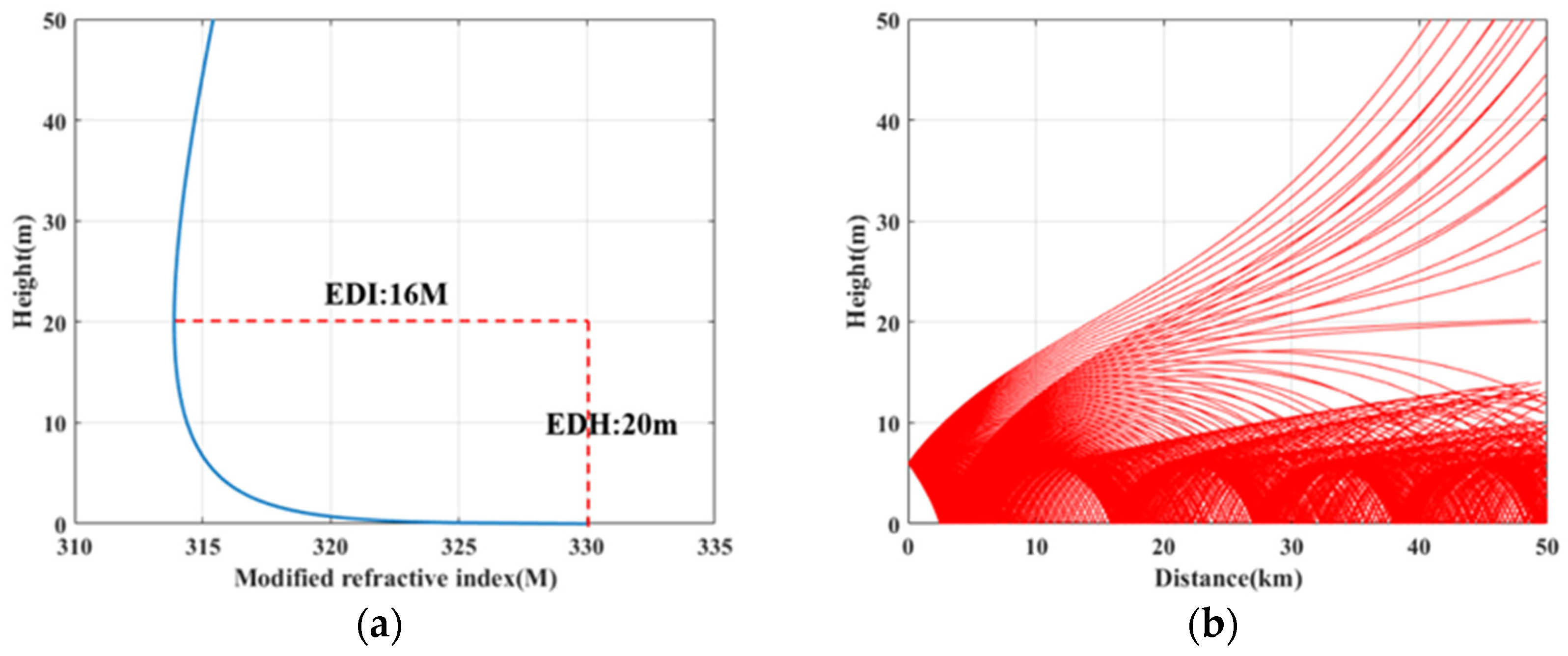
7], also called the ED profile. The evaporation duct height (EDH) is defined as the altitude of the lowest modified refractive index in an ED profile and represents the strength of the ED.
Almost all ED prediction models are based on the Monin–Obukhov similarity theory (MOST), but various models differ in the application of this theory. MOST assumes that the kinematics and thermodynamic structure of the steady and horizontally homogeneous near-surface layer with no radiation and no phase change depends just on the turbulence. As the ED is affected by the meteorological conditions at the sea surface, the EDH is usually determined by meteorological data observed from the ocean in the near-surface layer. By calculating the Monin–Obukhov-related parameters and using sea surface temperature (SST), surface pressure (SP) and atmospheric factors at a certain height, such as air temperature (AT), wind speed (WS) and relative humidity (RH), the Liu–Katsaros–Businger (LKB) model [
5] was first proposed to simulate the modified refractive index of the ED. On the basis of this framework, a series of ED models, including the Naval Warfare Assessment (NWA) model [
8], the Babin–Young–Carton (BYC) model [
9] and the Naval Atmospheric Vertical Surface Layer Model (NAVSLaM) [
10], were developed. Since then, there have been numerous studies on the temporal and spatial distribution of the ED [
2,
11,
12] and its characteristics [
3,
4,
13,
14,
15,
16,
17].
Babin et al. [
5] compared four ED models, NWA, Naval Research Laboratory (NRL), BYC and NAVSLaM, through a buoy experiment. As the ED profile obtained by direct measurement was used, the NAVSLaM was verified relatively close to the true value. The NAVSLaM is an ED prediction model proposed [
18] and improved [
10] by the US Naval Academy. It is worth noting that the improved NAVSLaM using the Grachev stability function [
19] has been theoretically shown [
11,
20] to have better performance in stable conditions where the ASTD is above 0 °C.
In combination with the radio-wave propagation model based on Maxwell’s law, the ED profile can be used to estimate EM-wave propagation in the troposphere. Several EM-wave propagation models based on numerical solutions, such as the ray-tracing model [
21], the parabolic equation (PE) model [
22] and the hybrid model [
23,
24], have been proposed and continuously developed. However, these models have different advantages in different usage scenarios. The PE model gives a full-wave solution for the field in the presence of range-dependent environments [
25] and has frequently been used to calculate the EM-wave path loss (PL) over the oceans. In recent years, with the development of ED models [
6,
7,
10,
26] and radio-wave propagation models [
23,
27,
28], it has become possible to study the OTH propagation over long periods, large areas and complex marine environments.
Rainfall is an important part of the water circulation and a common phenomenon at sea. Owing to global climatic change [
29,
30,
31], rainfall events have increased in recent years over the SCS [
32]. Wang et al. [
33] analyzed the high-resolution rainfall data for the tropical and subtropical areas of the Pacific Ocean, the Indian Ocean and the Atlantic Ocean. The results showed that the number of days with rainfall at sea is about 45.2%, which is dominated by intermittent rainfall that has a relatively high probability of occurrence from 04:00 to 15:00.
OTH transmission of EM waves at sea makes a communication link more susceptible to rainfall. Land experiments [
34,
35,
36,
37] have indicated that EM waves can be attenuated by rainfall. Specifically, the attenuation caused by rainfall is due to a mixture of the properties of the raindrops and changes in the atmospheric environment [
38,
39]. Moreover, attenuation owing to the nature of the rainfall is related to its intensity and spectral density [
35,
36]. The influence of meteorological factors during rainfall have been verified by several studies [
40,
41]. EM waves have a similar attenuation effect when propagating over sea owing to the physical mechanism of the rainfall. However, EM waves are also affected by the ED when propagating over sea, especially near the sea surface.
Recent studies have revealed a strong connection among the meteorological parameters, the atmospheric duct and the rainfall. Ma et al. [
42] found that rainfall has substantial effects on the sea surface, including a decrease in salinity and a rougher sea surface, which further influence the L-band sea surface emissivity. A study by Torri and Kuang [
40] showed that contrary to what was previously thought, the main source of water vapor in moist patches was surface latent-heat fluxes, not rain evaporation. Zhi et al. [
43] analyzed the interdecadal variation of autumn rainfall in western China and its relationship with atmospheric circulation and sea surface temperature anomalies. Liu et al. [
44] found that the inversed echo data from their proposed inversion model did not agree with the measurements in space owing to the influence of precipitation targets on the measured echo data. A slant path rain attenuation (RA) model was proposed by Dinc and Akan [
45] and was used to study the amount of rain loss from a specific duct and communication parameters. The simulated results show an attenuation of rainfall on the beyond-line-of-sight communication link, which is in line with our studies. However, the EDH during rainfall needs to be investigated.
The above studies of rainfall emphasized the influence of rainfall on meteorological parameters and the efficiency of communication in the duct layer during rainfall. However, the characteristics of atmospheric factors and the PL of OTH propagation during rainfall are still unknown. Moreover, the effects of rainfall on ED through the atmospheric changes need to be investigated.
In this paper, the effects of rainfall on the propagation characteristics of EM waves are studied, taking into consideration the influence of RA and the ED. Firstly, this study uses reanalysis data to analyze the temporal and spatial distribution of meteorological parameters in the South China Sea and the NAVSLaM to determine the distribution of the ED. The distribution of PL is given by the RA prediction model and the PE model. Then, the measurement data is used to verify the simulated results. In addition, some results of the measurements during different periods and similar studies are discussed. Finally, the effects of rainfall of EM waves are analyzed.
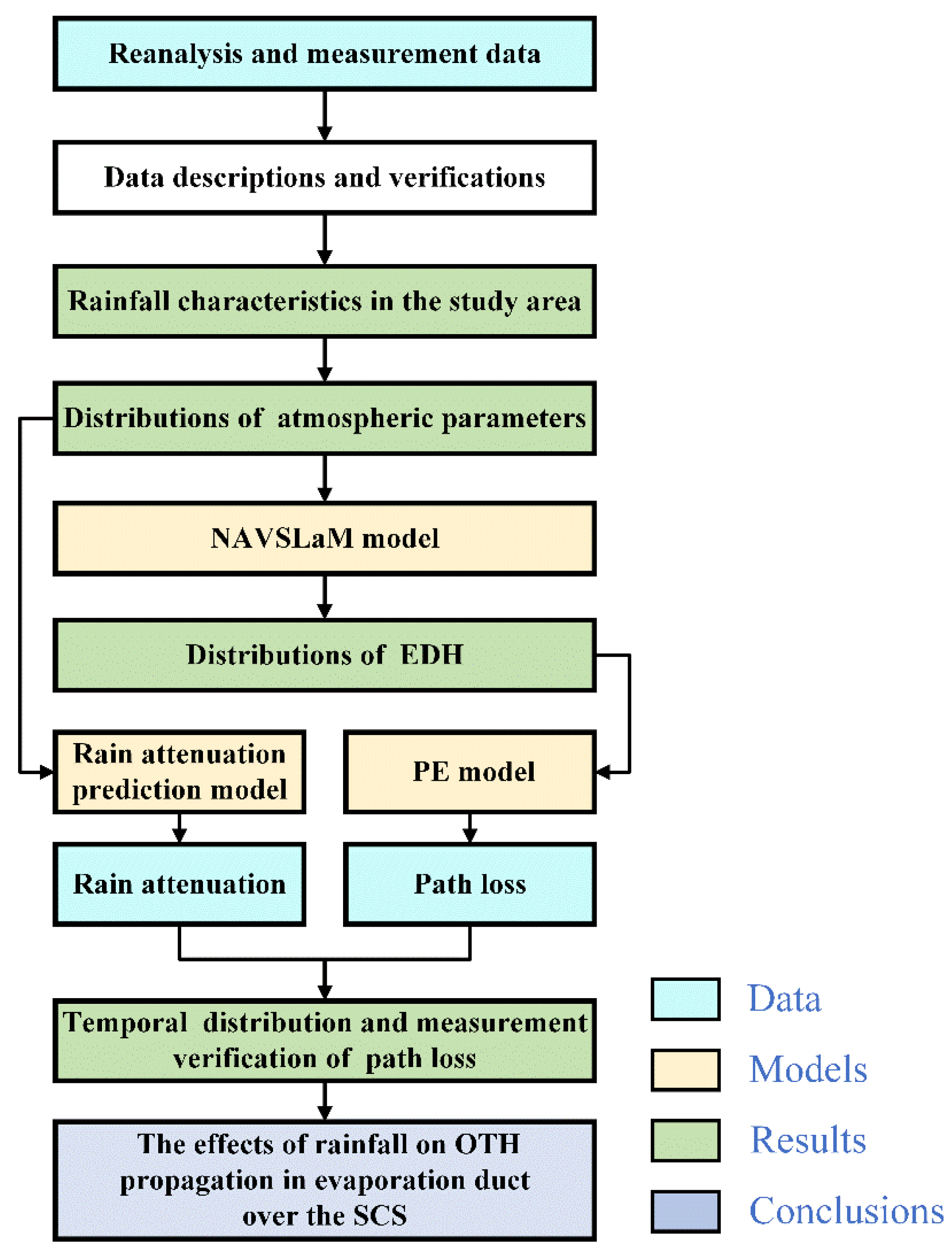
A research flowchart of this study is shown in
Figure 1. The study area, methods and datasets are introduced in this section. In
Section 3.1, the characteristics of annual rainfall in the study area and the distribution of rainfall density during the study period are introduced. In
Section 3.2, the temporal and spatial distributions of several meteorological parameters are summarized, including rain rate (RR), WS, AT, SST, RH and air–sea temperature difference (ASTD). The distribution of the EDH and the sensitivity of the EDH to meteorological parameters are analyzed in
Section 3.3. The simulated RA and PL are given in
Section 3.4. The PL temporal distribution and measurement verification are also given in this section. The additional three experiment results and the effects of RR and total rainfall on OTH propagation are discussed in
Section 4. The conclusions are given in
Section 5.
3. Results
3.1. Rainfall Characteristics
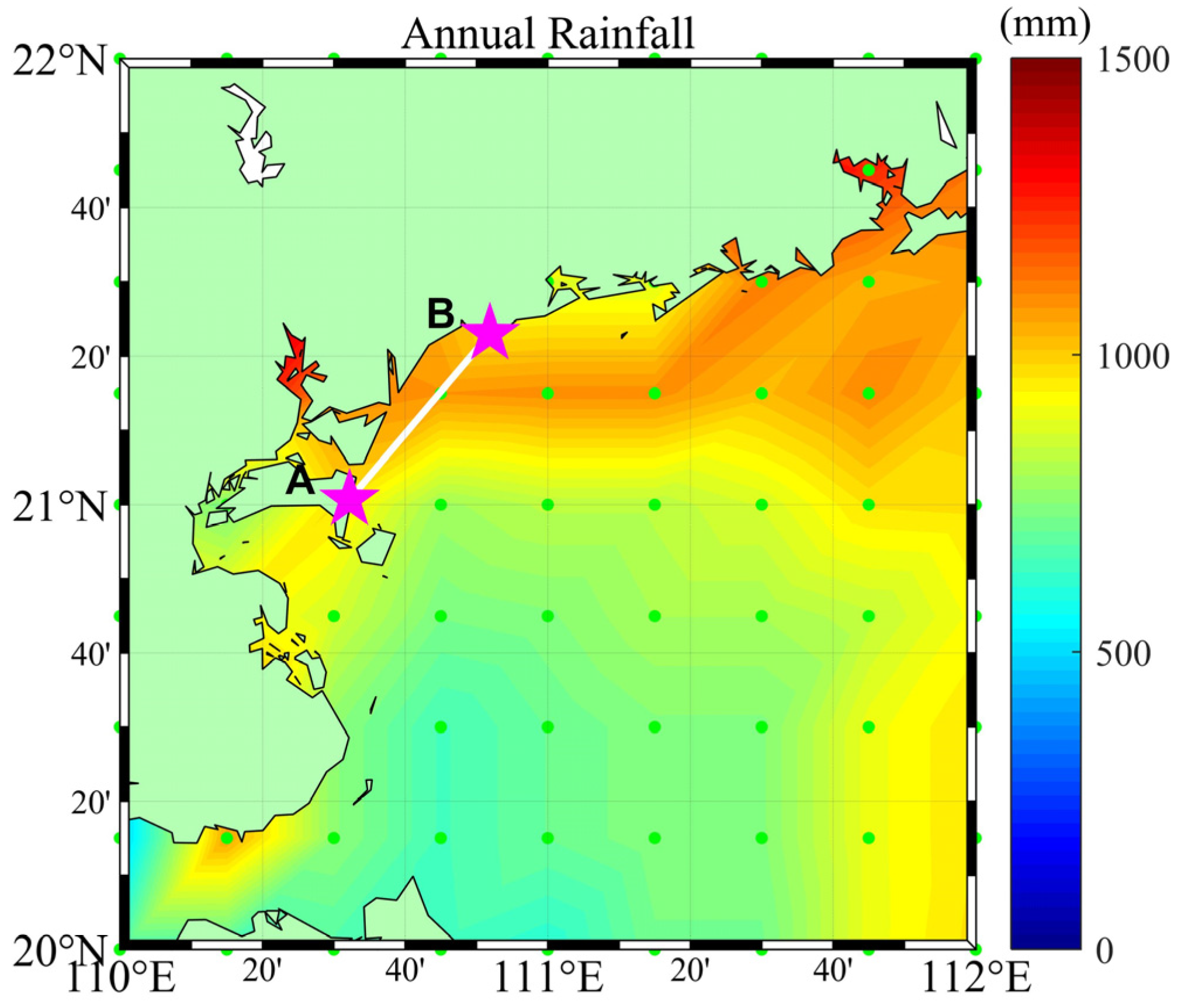
The annual RR in 2021 in the study area is shown in
Figure 9. Owing to monsoons [
67] and typhoons [
68], the RR was relatively high in the study area and the annual rainfall was more than 500 mm in the most areas. The monsoon from the ocean is more likely to result in rain at the coast. In particular, at latitudes above 21°N, the annual rainfall reached up to 1500 mm. Rainfall causes changes in the atmospheric environment and ocean parameters such as AT, SST, RH and WS [
69,
70].
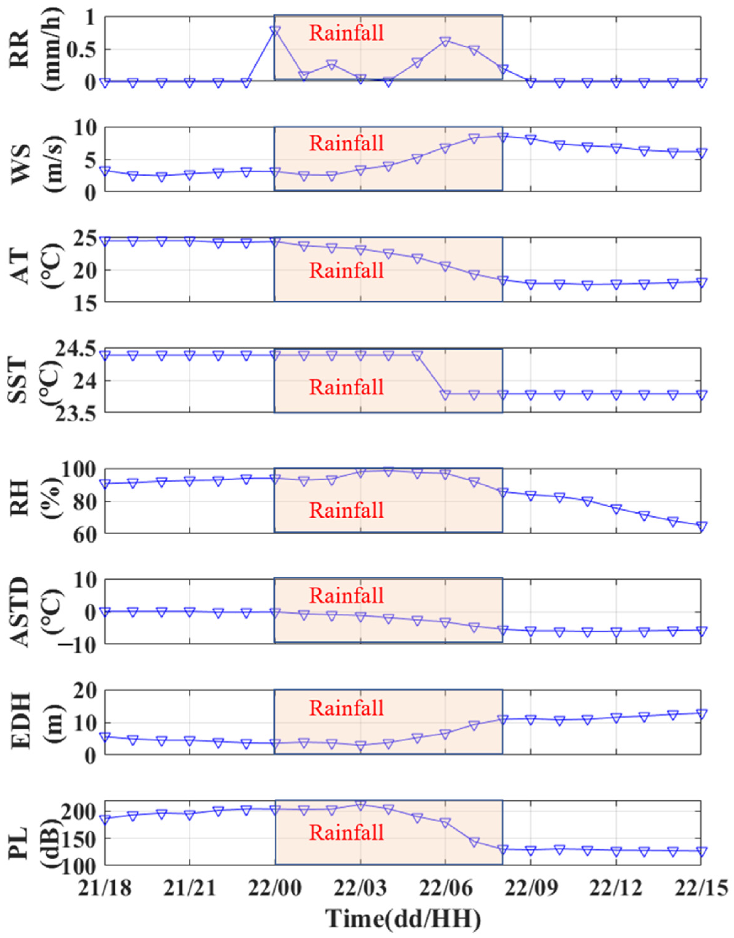
The study period from 18:00 on 21 November 2021 to 16:00 on 22 November 2021 (UTC+8) was divided into three parts, including the period before, during and after the rainfall. The rainfall lasted for a total of 9 h, causing changes in WS, AT, SST, RH, ASTD, EDH and PL, according to the records. At the beginning, the rainfall density reached the maximum of 0.79 mm s−1 at 0:00 on 22 November 2021. Then, the rainfall density decreased to 0.01 mm s−1 at 4:00 on 22 November 2021. After that, the rainfall density increased to 0.63 mm s−1 at 6:00 on 22 November 2021 and began to decrease till disappeared after 8:00 on 22 November 2021.
3.2. Atmospheric Parameters
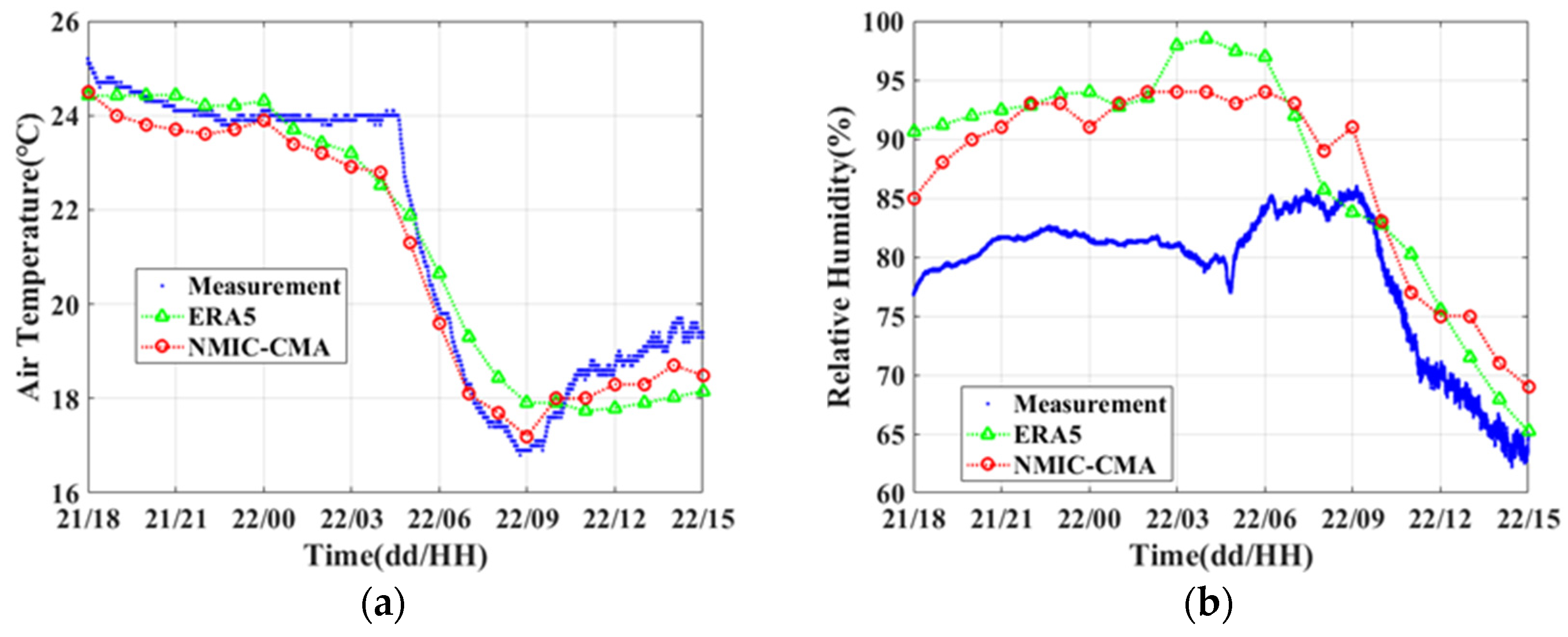
Figure 10 shows the evolution of the RR, WS, AT, SST, RH, ASTD, EDH and PL during the study period at position C. The rainfall period is indicated by a light pink box from 0:00 to 08:00 on 22 November 2021. The units of these parameters are the same as in
Table 1. In general, the EDH is insensitive to the changes in SP [
71], thus, the SP is not mentioned in the rest of this article.
Before the rainfall, the WS was lower than 3.4 m s−1, the AT was higher than 24.2 °C and the SST was steady at 24.38 °C. The RH was over 91% and had been increasing from 18:00 on 21 November. The ASTD decreased from 0.03 °C to −0.17 °C, which means that the atmospheric stability changed from stable conditions to unstable conditions.
During the rainfall, the RR decreased to nearly 0 mm s−1 at 04:00 and then increased to 0.6 mm h−1 at 06:00. The WS increased from 3.1 m s−1 to 8.5 m s−1. The AT decreased to 18.4 °C. The SST dropped by 0.59 °C between 05:00 and 06:00. The RH first increased to a maximum value of 98.53% at 04:00 and then began to decrease. The ASTD decreased to −5.4 °C.
After the rainfall, the WS remained at a high level and slowly decreased to 6.0 m s−1 at 16:00. The AT remained at a low level, around 18 °C. The SST remained steady at 23.79 °C. The RH dropped from 85.7% to 63.7%. The ASTD remained at a low level, around −5.8 °C.
For the whole study period, the WS increased after the rainfall compared with that before the rainfall. The RH had been close to saturation before the rainfall. The RH, AT, SST and ASTD decreased after rainfall compared with that before rainfall. Unlike over land, there is no evidence for a decreasing precipitation event duration with increasing SST [
72]. As the specific volume of seawater is higher than that of the air, changes in the SST are slighter and slower than the changes in the AT when rainfall occurs. Furthermore, the correlation between evaporation and the ASTD is much stronger than that with SST [
73]. Hence, the AT and SST are combined into ASTD in the rest of this article.
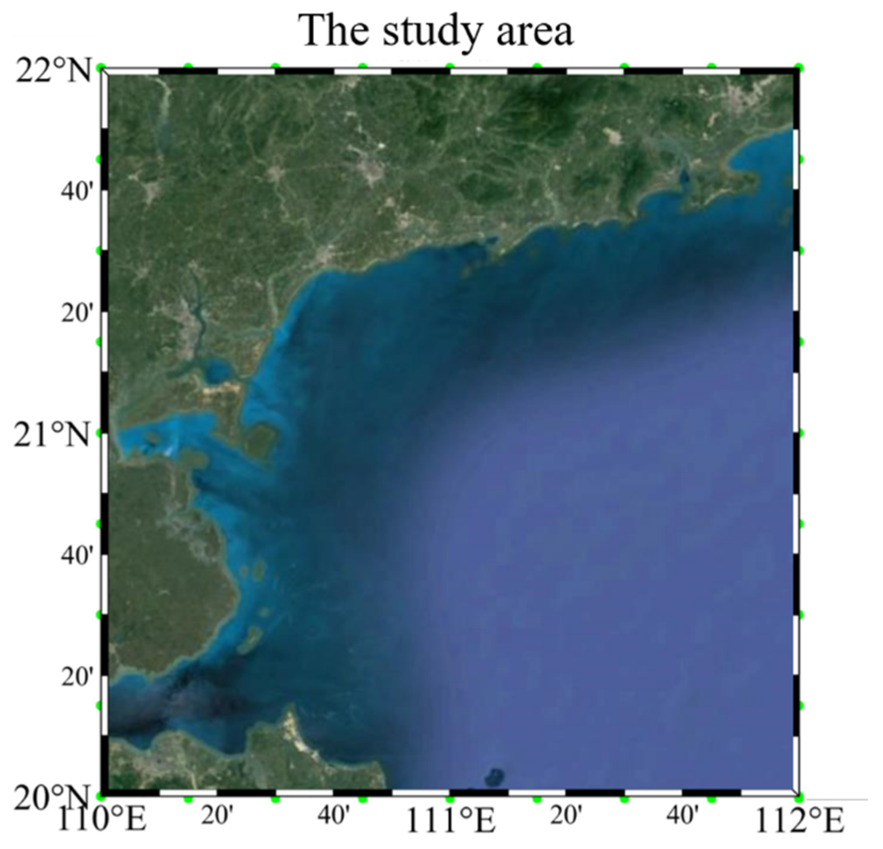
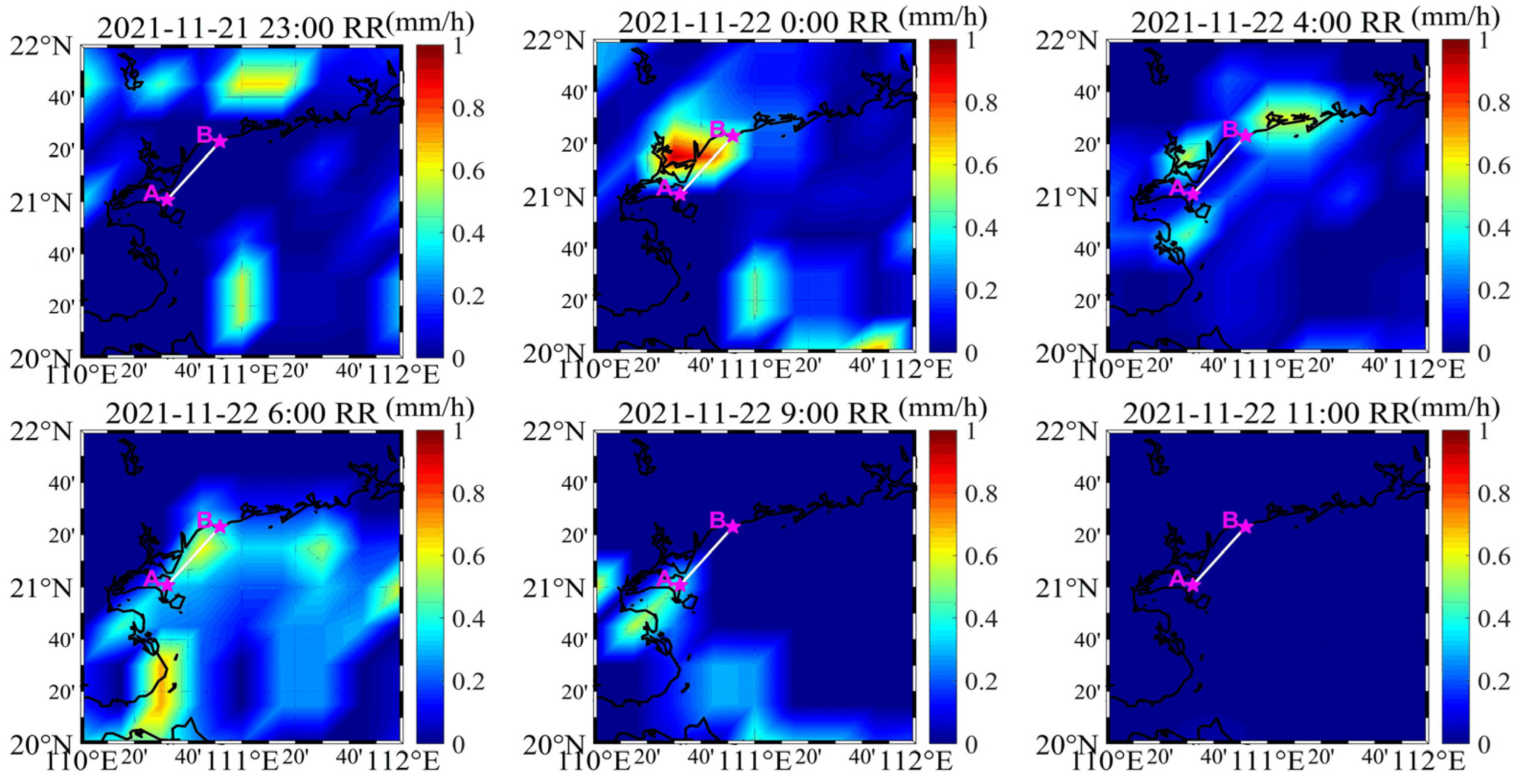
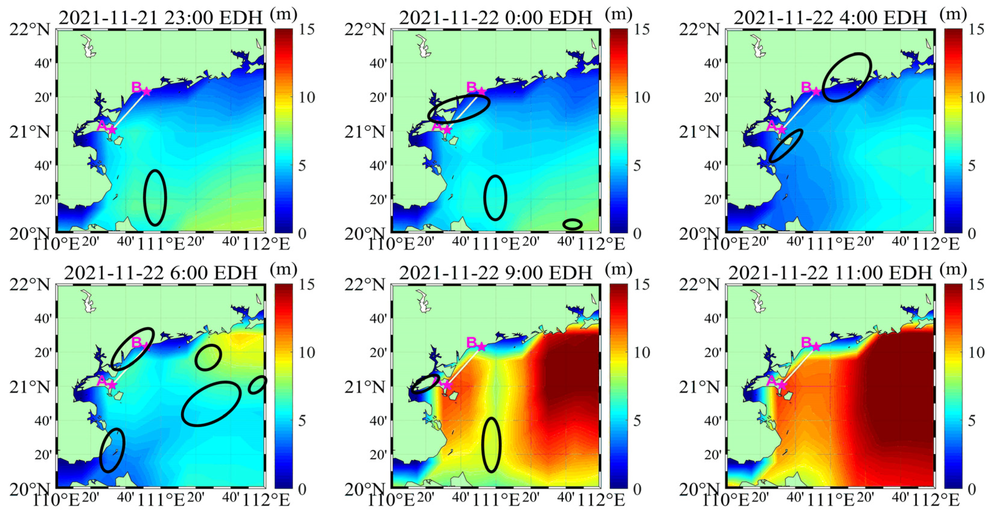
Rainfall often occurs over a large area, and the meteorological changes at a single location cannot accurately reflect the effects of rainfall. In addition, the ED distribution over a large area of the sea is also needed for the OTH propagation link. Therefore, six typical time points (23:00 on 21 November, and 00:00, 04:00, 06:00, 09:00 and 11:00 on 22 November) were selected to analyze the evolution of the regional meteorological parameters. The data were downloaded from the ERA5.
Figure 11 shows the spatial distribution of RR in the study area at the six times. The rainfall area almost covered the OTH propagation link between positions A and B at 00:00 and 06:00 on 22 November. There was a little rainfall around position B at 04:00 on 22 November and position A at 09:00 on 22 November.
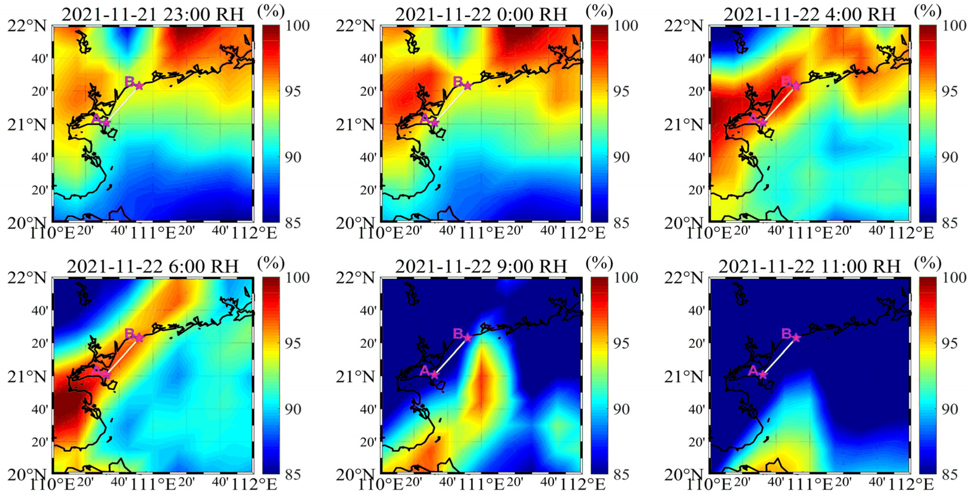
Figure 12 shows the spatial distribution of RH in the study area at the six times. The RH was relatively high around the coast before 06:00. The moist patches moved along the coastline from west to east at first, then moved towards the south.
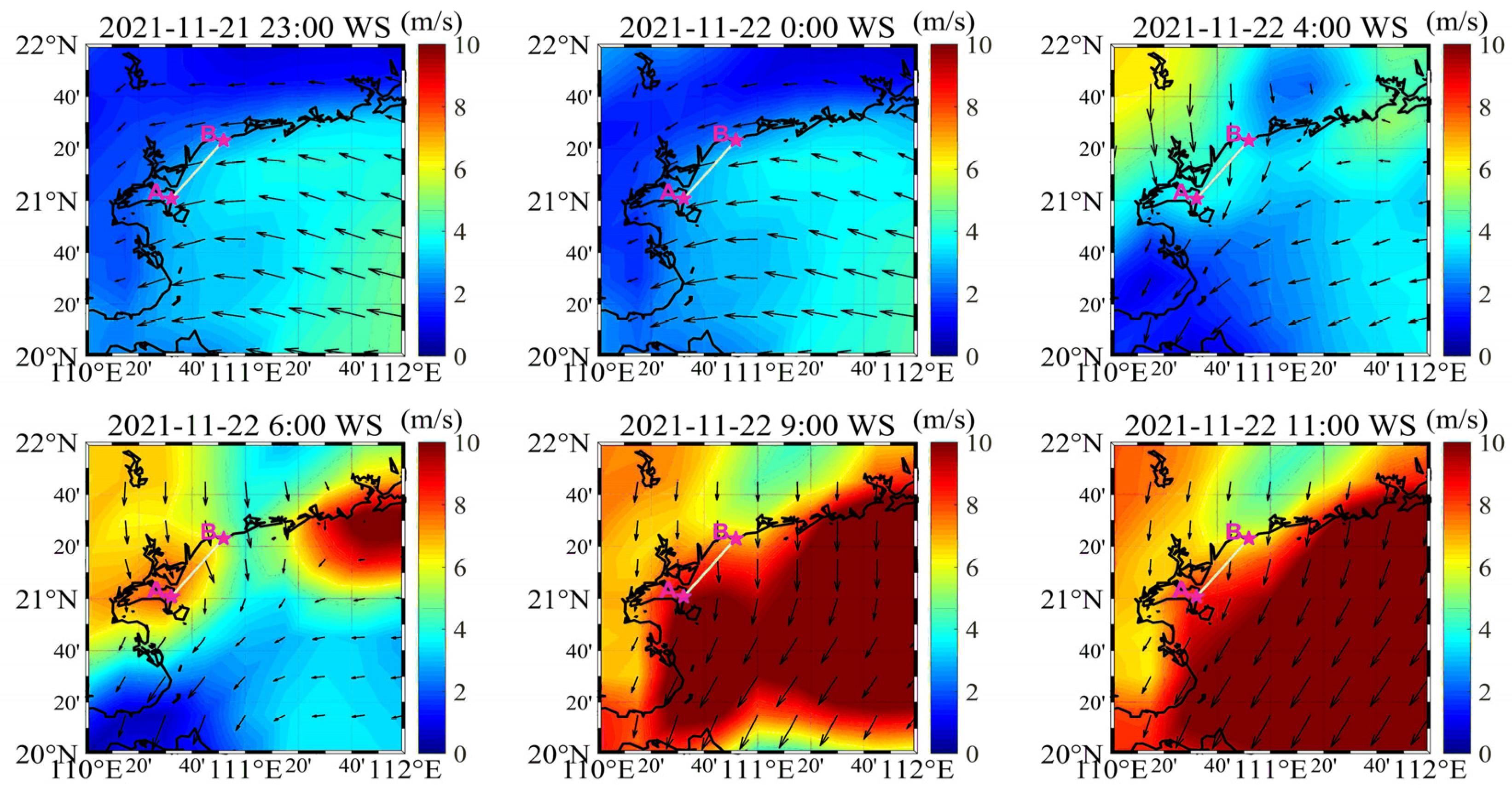
Figure 13 shows the spatial distribution of the WS and wind direction in the study area at the six times. The WS was less than 5 m s
−1 at the start. Then, strong winds over 10 m s
−1 appeared from the west coast and the east coast in the study area at 06:00 on 22 November and eventually met in the middle of the study area. The whole area was covered by strong winds after 9:00 on 22 November.
The wind came from the east and moved to the west, and the moisture from the evaporation of seawater was transported to the edge of the land by the wind, creating strong RH at the coast (
Figure 12). From 04:00 on 22 November, the wind turned toward the south, and the moist patches were transported to the south at the same time (
Figure 12).
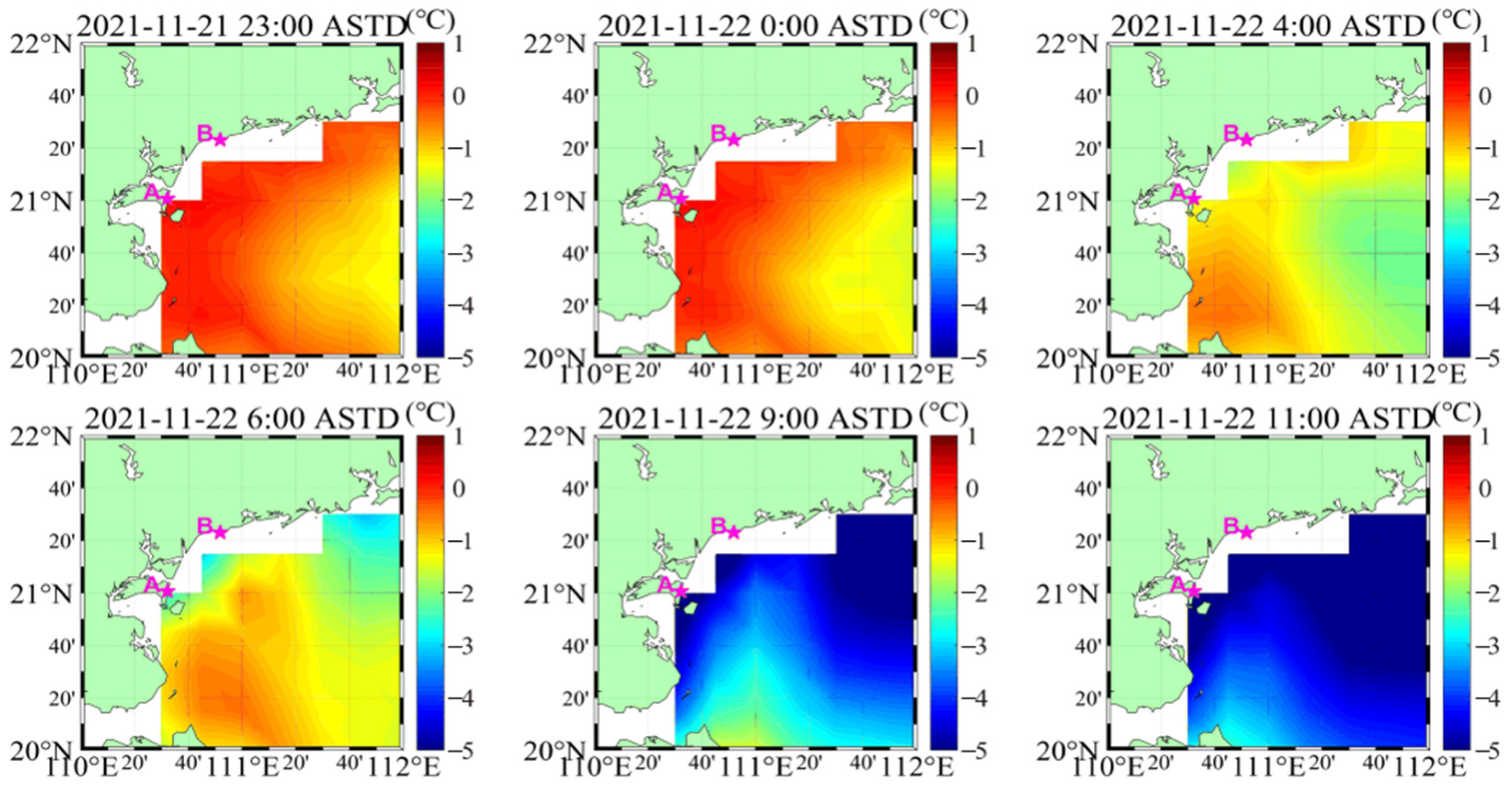
Figure 14 shows the spatial distribution of the ASTD in the study area at the six times. As shown in
Figure 14, the ASTD was higher than zero before 04:00 on 22 November in the areas close to the coast and lower than zero after 04:00 on 22 November. The ASTD became increasingly lower in the study area, especially after 04:00 on 22 November. An interesting find is that the atmospheric conditions were more unstable where the WS was stronger and vice versa. When the ASTD close to land was considered as the difference of land air and sea surface, the changes in the ASTD caused a sea–land breeze that eventually affected the wind direction.
In summary, rainfall occurred with a series of atmospheric processes. Under the effects of the sea–land breeze, the wind direction and WS changed immediately. Strong WS and the change in wind direction caused the moist patches to move during the rainfall, which eventually affected the RH. The RH at position C was almost saturated before the rainfall and unexpectedly decreased during the rainfall. The WS after rainfall was higher than that before rainfall and changed its direction during rainfall. The ASTD values changed from positive to negative near the coast under the effects of rainfall.
3.3. EDH Analysis
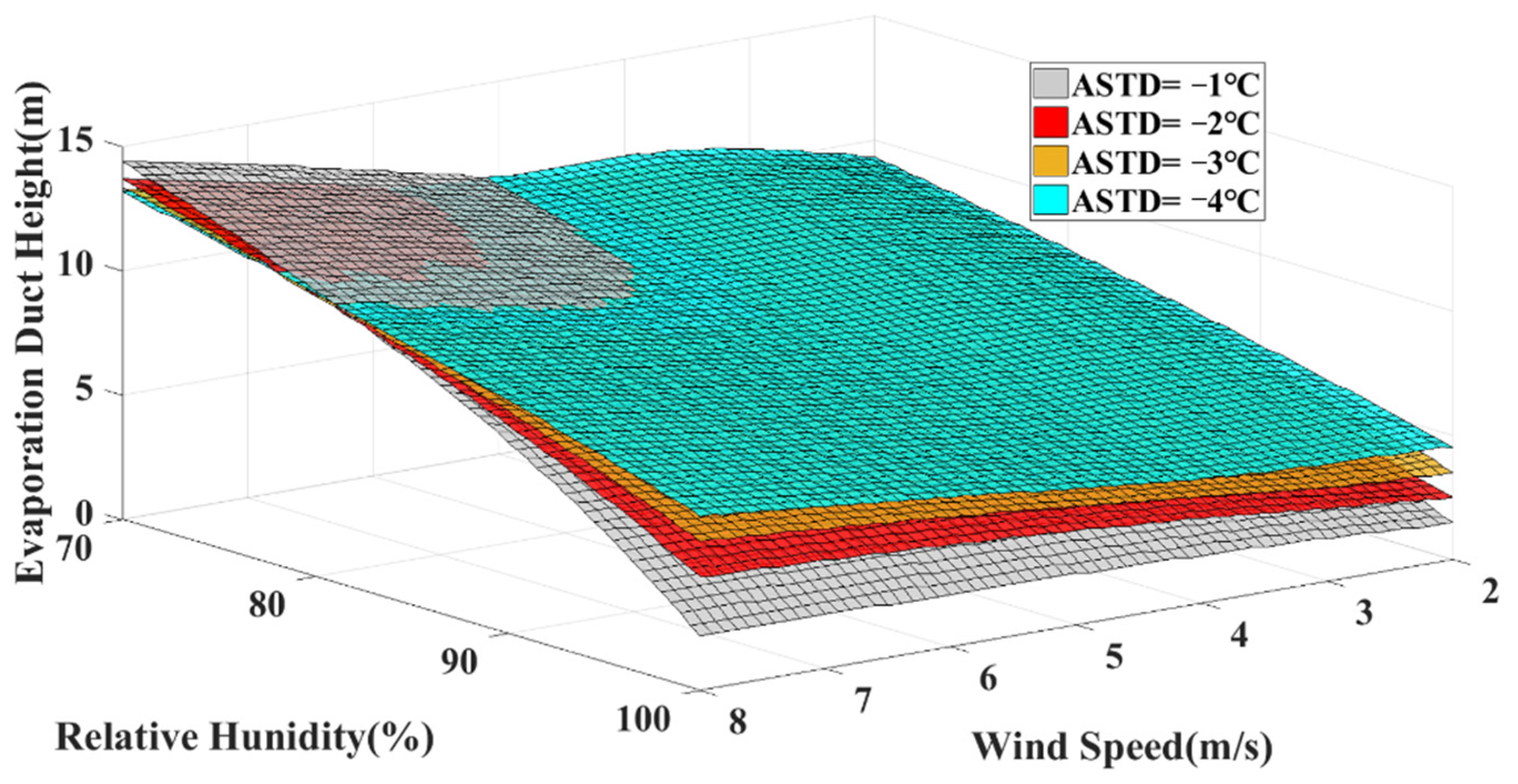
The NAVSLaM was used to study the sensitivity of the EDH to the ASTD, WS and RH (
Figure 15). The SST was 24 °C and the pressure was 1015 hPa, which are the average values in the study area. As seen in
Figure 15, a high EDH is usually accompanied by low RH and strong WS. Using the data in
Figure 15, the ranges of the EDH under different ASTD values are shown in
Table 3. The gradient of the EDH decreased with decreasing ASTD. When the RH was over 85% or the WS was under 5 m s
−1, the decrease in ASTD accelerated the changes in the EDH. Therefore, the increasing WS accompanied with the decreasing RH led to an increase of the EDH during rainfall; the growth rate of the EDH was inversely proportional to the value of the ASTD under this condition.
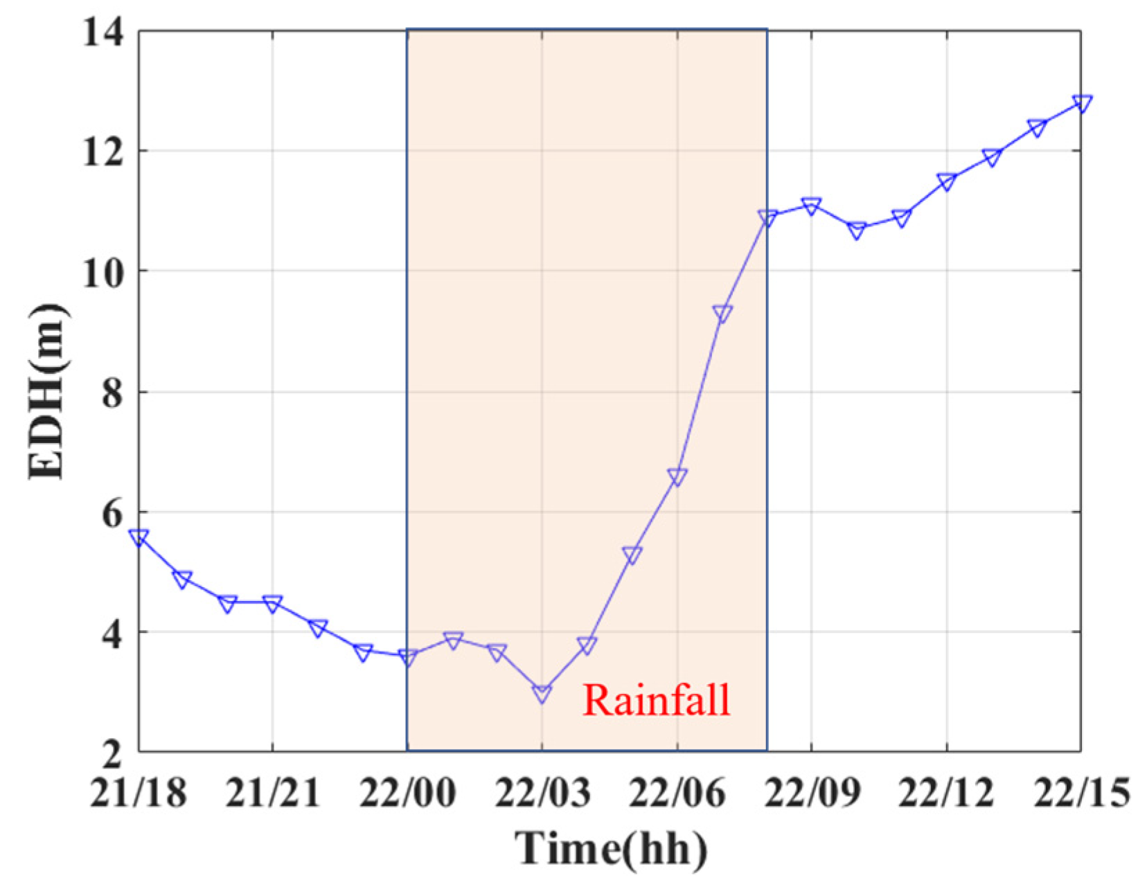
Figure 16 shows the evolution of the EDH during the study period at position C. The rainfall period is indicated by the light pink box from 00:00 to 08:00 on 22 November.
Before the rainfall, the EDH was at a low value and decreased in this period. The wind had already brought some moist patches into the area, leading to a high RH value.
During the rainfall, the EDH decreased before 03:00 on 22 November owing to the increasing RH. After that, the EDH increased for two reasons: the increasing WS and almost constant RH between 03:00 and 04:00 on 22 November and the decreasing RH accompanied by increasing WS after 04:00 on 22 November.
After the rainfall, the EDH continued to increase for a period of time. This is because the RH continued to decrease after the rainfall, and the WS was much higher than before the rainfall.
Figure 17 shows the spatial distribution of EDH in the study area at the six time points. In most ellipses, the EDH was significantly lower than that in the surrounding areas without rainfall. Moist patches can apparently affect the distribution of the EDH. In particular, at 09:00 on 22 November, the high RH caused a low-EDH region around 111°E during rainfall.
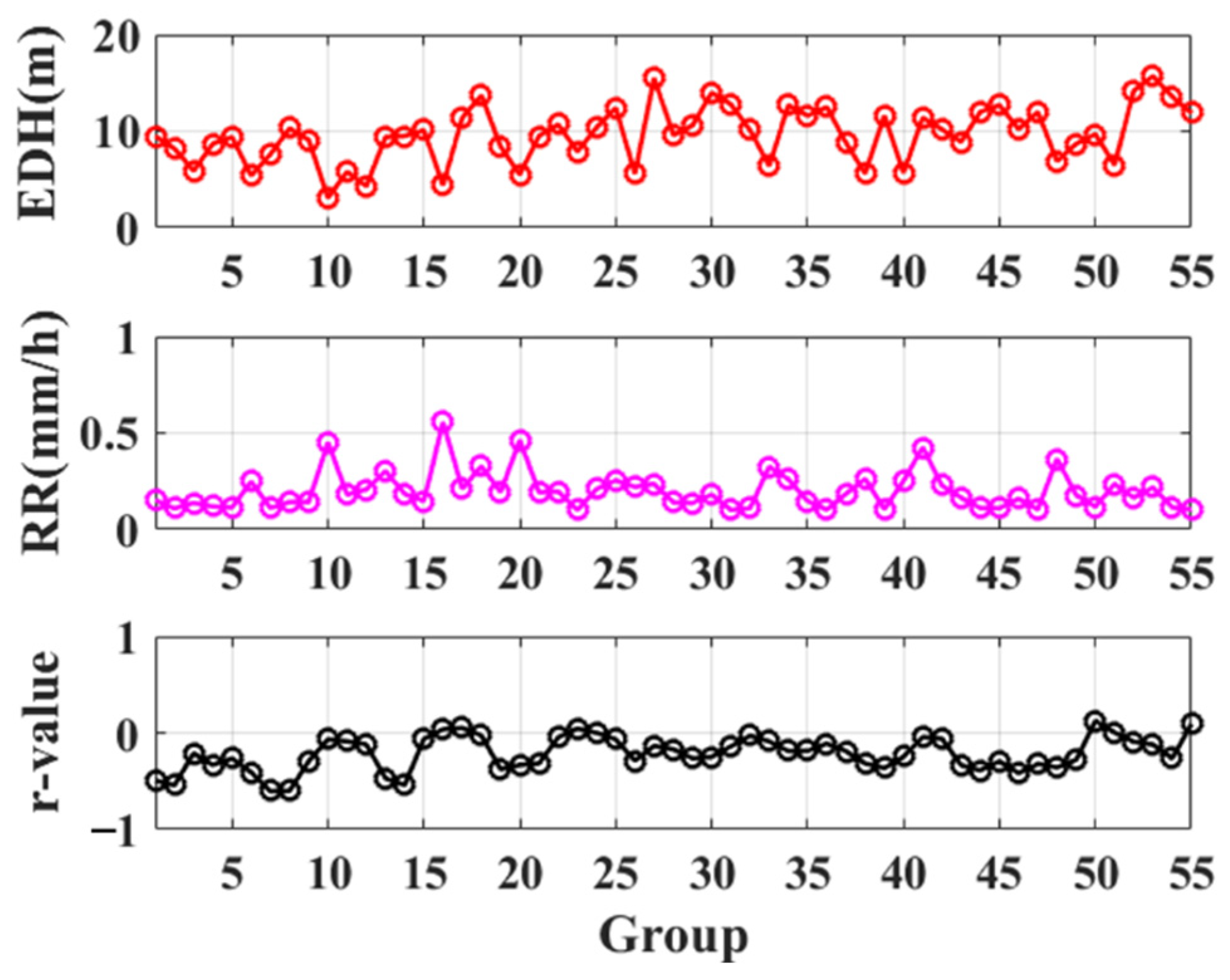
The Pearson correlation coefficients of the EDH and RR are shown in
Figure 18. After removing the data on land and the data without rainfall, there were 833 samples. The preprocessed data was divided into 55 groups. Every 16 samples were formed in one group. The last group with insufficient data was supplemented by the samples of the previous group. It can be seen from
Figure 18 that there is a negative correlation between RR and EDH. Most of the correlation coefficients are lower than 0. A small number of points close to 0 may be affected by other complex marine environments, such as the sea–land breeze. The average Pearson correlation coefficient of the EDH and RR is −0.18, which shows a weak negative correlation.
In summary, rainfall causes changes in the atmospheric environment and ocean parameters that eventually affect the EDH. In the study area, the EDH decreased during rainfall in most cases. In the study period, the EDH was low before and during rainfall owing to the high RH and low WS. However, the EDH increased during rainfall when the WS was becoming stronger, and the moist patches brought by rainfall were moved. The EDH remained higher after the rainfall owing to the lower RH.
3.4. PL Analysis
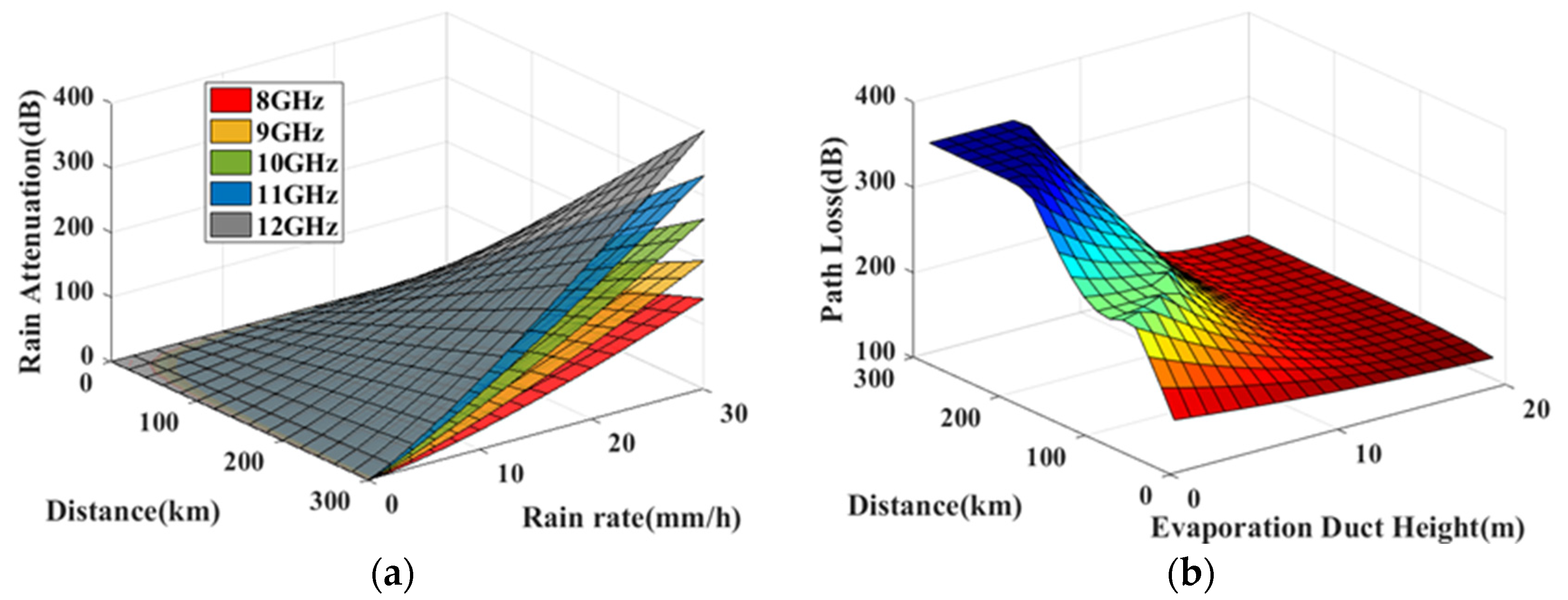
In this section, RA and PL are estimated by the ITU calculation model and the PE model, respectively. The simulation parameters used in the PE model are shown in
Table 4. The effects of the ED and RA on the propagation of EM waves at sea is shown
Figure 19.
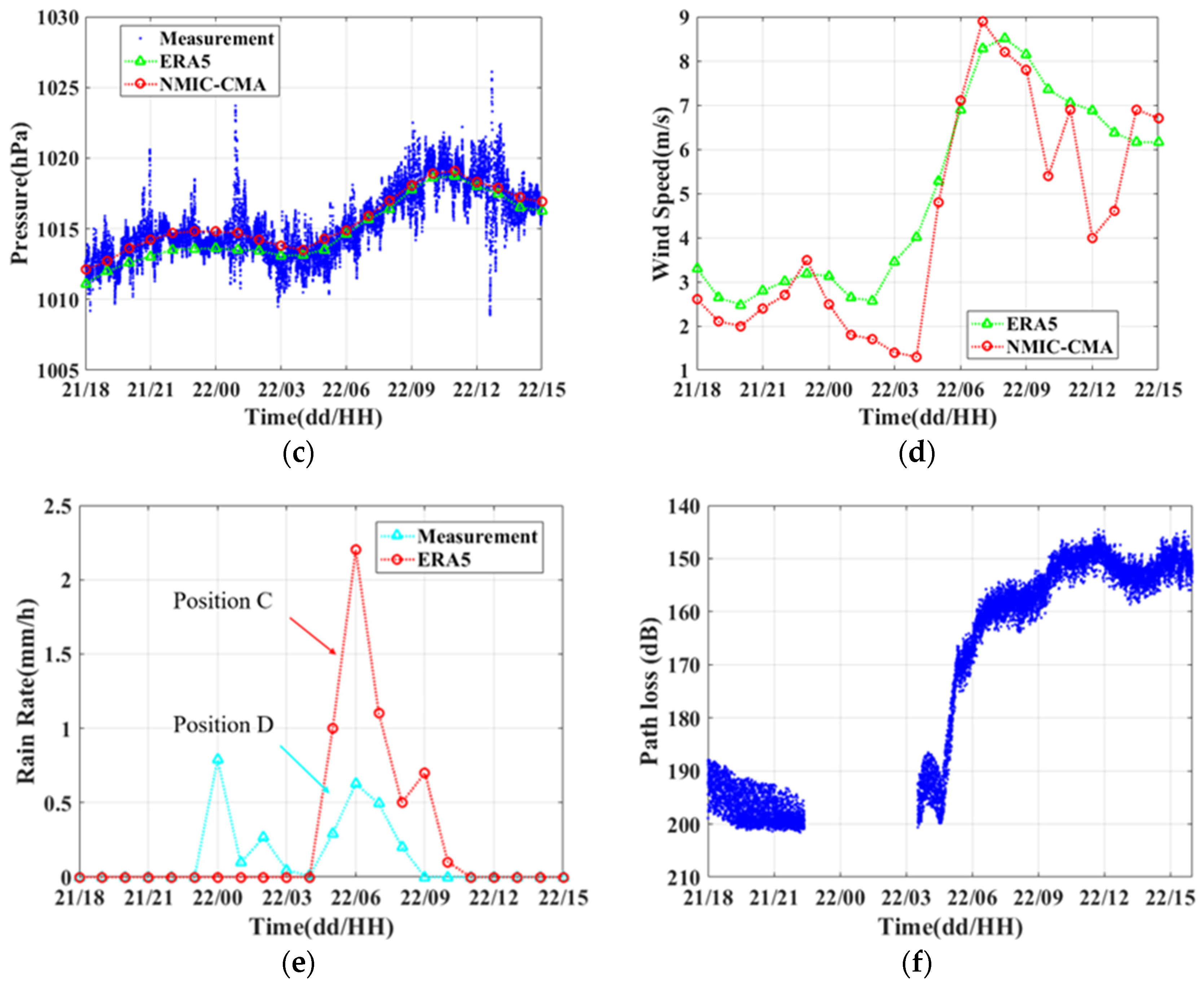
As shown in
Figure 19a, RA is a function of EM-wave frequency, distance through the rain region and rainfall intensity (equal to RR in an hour), according to the ITU model. It is evident that when the frequency is constant, RA generally increases with increasing distance and RR. When the frequency changes, a decrease in frequency leads to a marked decrease in RA. When RR is less than 5 mm h
−1, the maximum attenuation of the EM waves in the range of 8–12 GHz caused by the rainfall is 0.16 dB km
−1.
Using several samples of ED profiles generated by the NAVSLaM, the PL within 300 km in
Figure 19b shows an origami-crane-like structure. The peak of the PL difference for the mean distance surpasses 0.69 dB km
−1. When the EDH is less than 5 m and the distance is below 50 km, the PL is less than 180 dB. However, once the distance reaches 60 km with an EDH less than 5 m, the PL exceeds 200 dB. In contrast, when the EDH is more than 11 m, the PL of the EM-wave propagation to 300 km does not exceed 200 dB.
Furthermore, the effect of the ED on PL reaches 0.69 dB km−1 on average, which is 4.3 times stronger than the maximum RA (0.16 dB km−1), when the rainfall is less than 5 mm h−1. The propagation of EM waves over the sea is still mainly affected by the ED. Thus, the marine EM-wave systems should be suitable for using the optimal frequency band for the best ED during rainfall under 5 mm s−1.
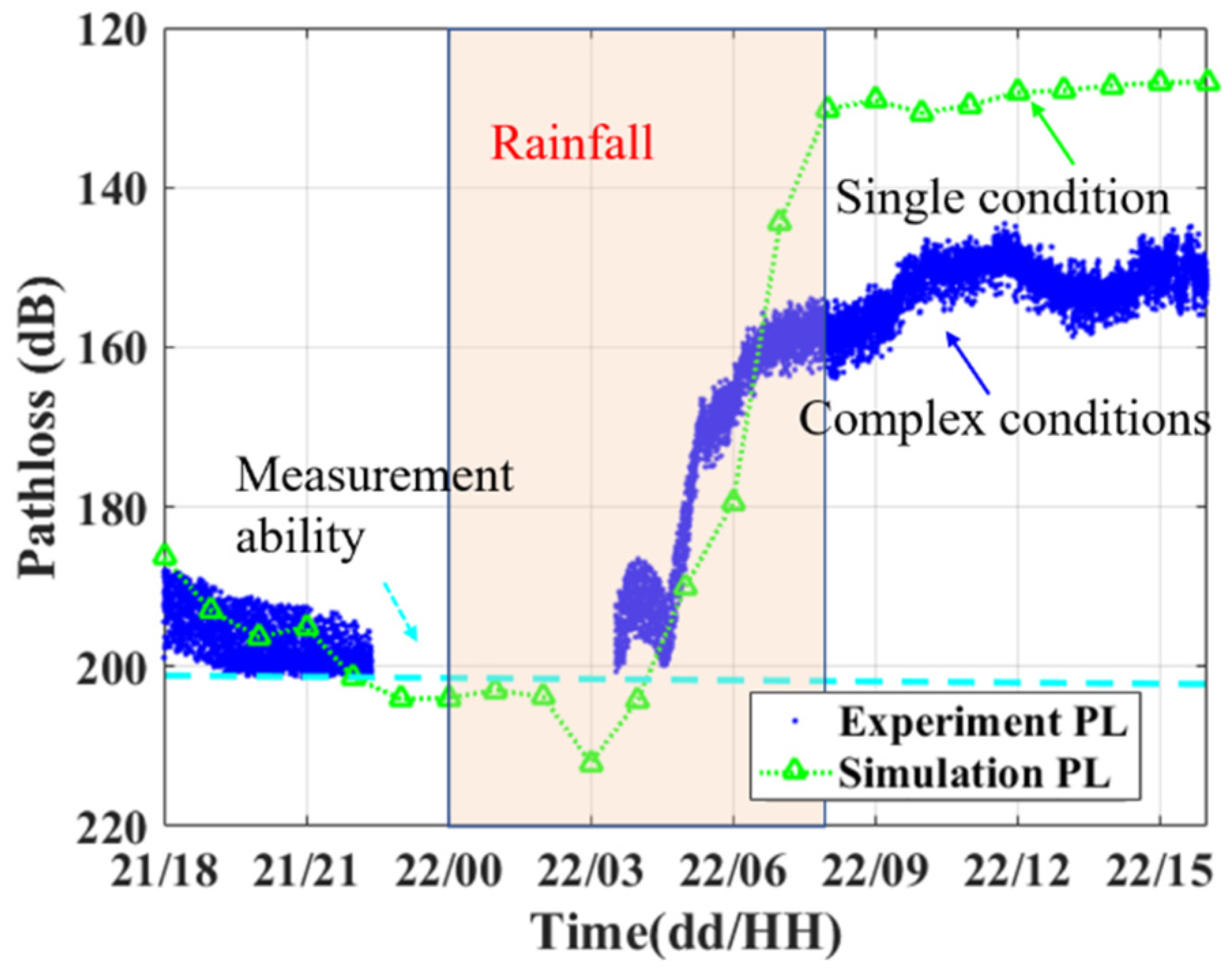
Figure 20 shows the simulation and measurement curves of the EM-wave PL in the ED during rainfall. The EM wave was transmitted from Jizhao Bay and was received at Donghai Island after propagating 53 km. The received signal level was recorded every four seconds by a computer. The experimental configurations are shown in
Table 5. The frequency of the EM wave is 8.0005 GHz. Although the simulation PL included the RA during rainfall, the RA according to the ITU is less than 5 dB. In fact, the PL difference in
Figure 20 is over 50 dB and rapidly changes within an hour.
It can be seen in
Figure 20 that the simulated PL is strongly consistent with the measured PL, and their trends are similar. The simulated PL shows the opposite trend to the EDH (
Figure 16). The simulated PL increased to a maximum value of 212.1 dB at 03:00 on 22 November. After that, the increase in the EDH resulted a decrease of the simulated PL, until the simulated PL decreased to 130.1 dB at 08:00 on 22 November during rainfall. The measured PL gradually decreased to 157.6 dB at 08:00 on 22 November and decreased slowly for a period of time after rainfall. The movement of moist patches caused by a sea–land breeze brought a 7.1 m increase of EDH and a 42.4 dB decrease of PL, which was an abnormal phenomenon during rainfall.
The difference between the measured PL and the simulation PL after 07:00 on 22 November was mainly produced by the OTH link, where only one grid point at the position C was used, rather than the range-dependent modified refractivity profiles along the OTH link. Moreover, complex conditions such as inhomogeneous ED, waves and surface roughness would affect the simulation PL.
In summary, the effect of RA on OTH propagation owing to rainfall is much less than the effect of the ED when the RR is under 5 mm s−1. The PL is at a high value before and during rainfall but decreases during rainfall when the WS increases and the RH decreases. Furthermore, the PL decreases after rainfall when the RH continues to decrease.
4. Discussion
Both the RR and total rainfall can produce a great influence on the meteorological factors over the sea. Therefore, this section discusses the effects of RR and total rainfall on OTH propagation and verifies the results in
Section 3.
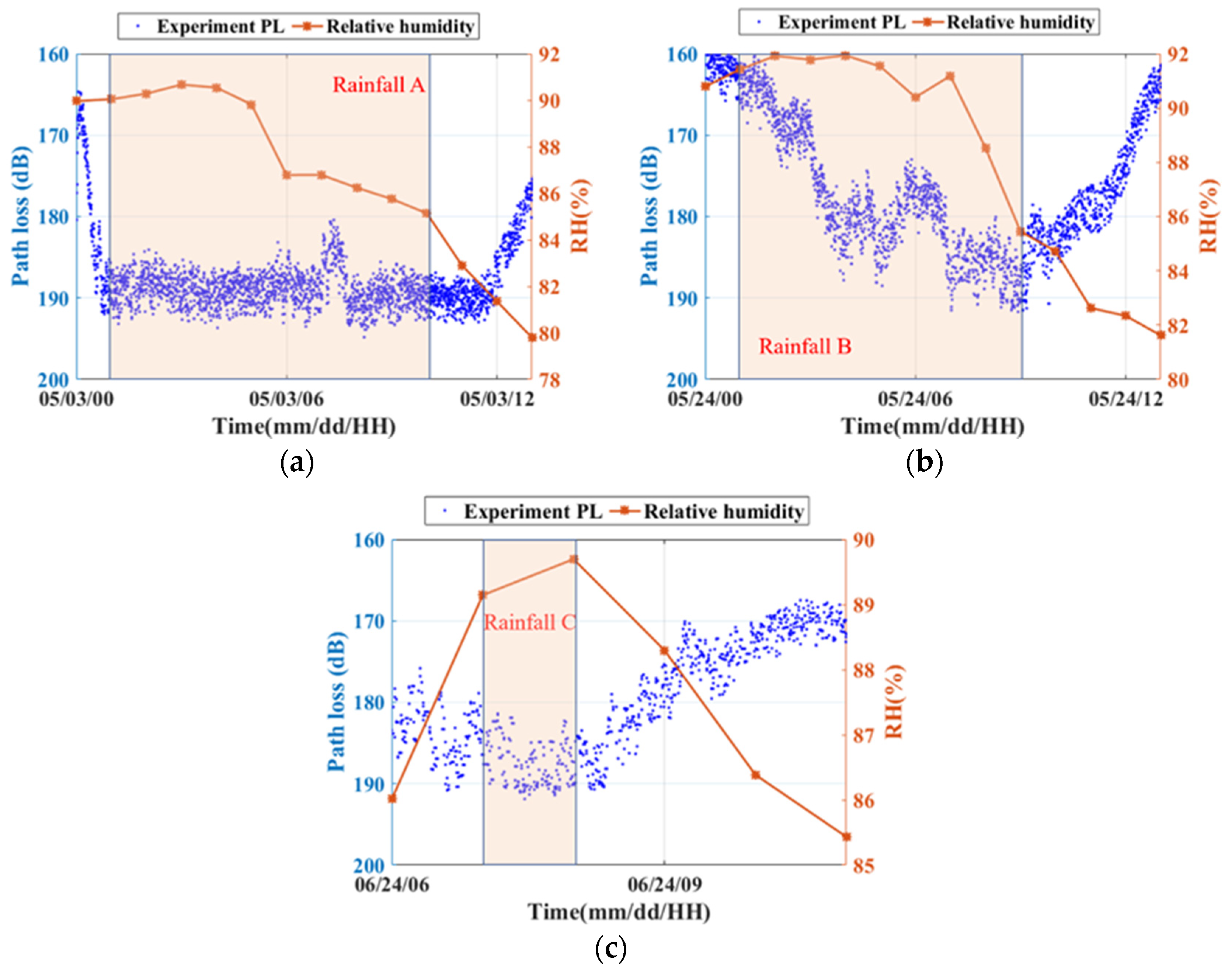
To further verify the conclusions, the three additional experiment results are given in
Figure 21. The experiment was also held in the SCS in 2021 with different equipment of an omnidirectional antenna at the receiver. The three rainfall events are chronologically labeled as Rainfall A, Rainfall B and Rainfall C.
The rainfall brought the near-saturated humidity in
Figure 21a and an increasing RH in
Figure 21b, causing a higher PL. The lower RH after rainfall caused PL below 180 dB. However, these three observations did not show a decreasing PL during rainfall due to the absence of the direction change of the sea–land breeze. It is worth noting that the rainfall intensity during all three rainfall periods did not exceed 5 mm h
−1, which means the EDH was still the main impact factor of the OTH propagation link, rather than the RA.
In summary, these three additional experiment results showed that the PL decreased to a lower value with the high humidity, which is consistent with the results of
Section 3.
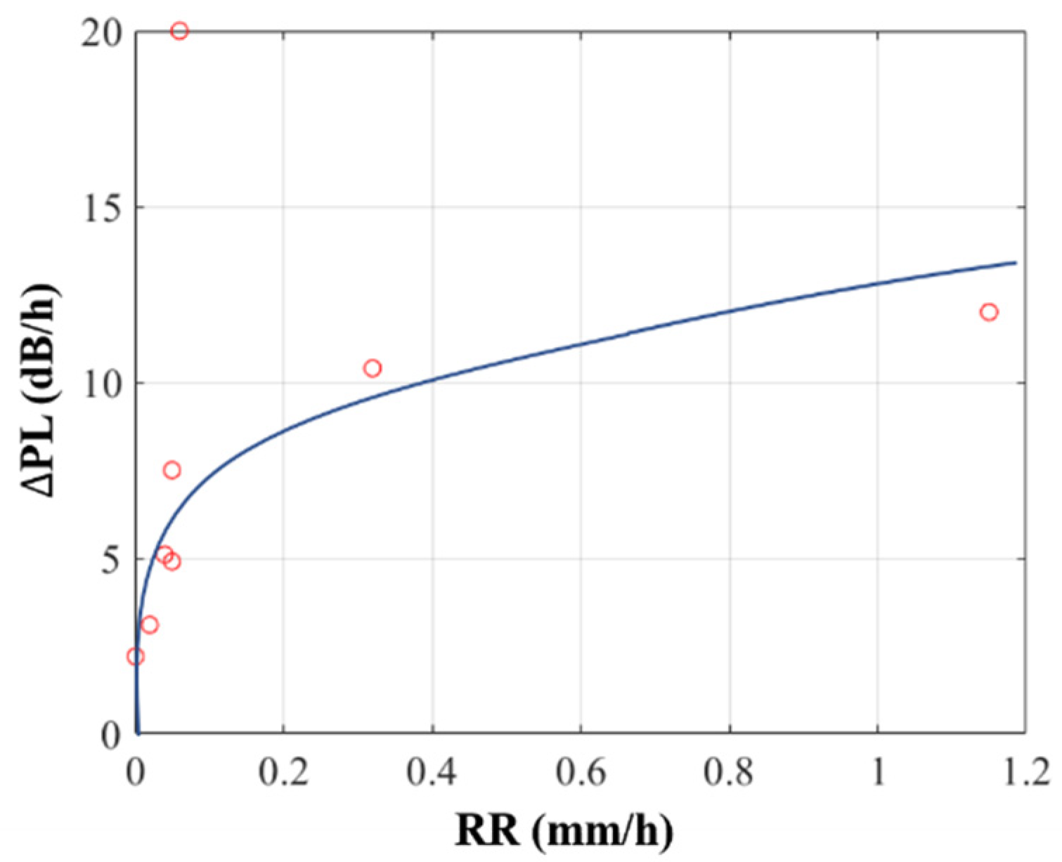
With the data of RR and PL from the additional experiment results,
Figure 22 shows the relationship between RR and ∆
PL. The ∆
PL is the hourly increased value of PL and is calculated by:
where
represents the hourly averaged PL, and
represents the hourly averaged PL one hour before
.
As
Figure 22 shows, the fitting curve is a logarithmic function of ∆
PL and RR. When the RR is over 0.5 mm h
−1, the ∆
PL exceeds 10 dB h
−1. According to this trend, ∆
PL will eventually increase to about 18 dB h
−1 and no longer change with RR, which needs to be verified by more observations.
To discuss the effects of total rainfall on OTH propagation, the parameters of the additional experiment results during rainfall are given in
Table 6. The total rainfall during Rainfall A is 2.3 mm, which is the highest rainfall of the three experiments with the highest average PL (189 dB). The total rainfall during Rainfall B is 0.7 mm, which is the lowest rainfall of the three experiments with the lowest average PL (178 dB). Although the duration of the rainfall is different, the average PL is higher when the total rainfall is higher. This means total rainfall can be an influential factor of PL on OTH propagation.
In summary, both RR and total rainfall can be the influential factors of PL on OTH propagation. The fitting curve of ∆PL and RR is a logarithmic function. According to the trend of the curve, the maximum of the ∆PL will be about 18 dB h−1, which needs to be verified by more observations. The total rainfall also shows a negative influence on average PL during rainfall in which the average PL is higher when the total rainfall is higher.


 ,
, 


