Blind Restoration of Atmospheric Turbulence-Degraded Images Based on Curriculum Learning

Abstract

Atmospheric turbulence-degraded images in typical practical application scenarios are always disturbed by severe additive noise. Severe additive noise corrupts the prior assumptions of most baseline deconvolution methods. Existing methods either ignore the additive noise term during optimization or perform denoising and deblurring completely independently. However, their performances are not high because they do not conform to the prior that multiple degradation factors are tightly coupled. This paper proposes a Noise Suppression-based Restoration Network (NSRN) for turbulence-degraded images, in which the noise suppression module is designed to learn low-rank subspaces from turbulence-degraded images, the attention-based asymmetric U-NET module is designed for blurred-image deconvolution, and the Fine Deep Back-Projection (FDBP) module is used for multi-level feature fusion to reconstruct a sharp image. Furthermore, an improved curriculum learning strategy is proposed, which trains the network gradually to achieve superior performance through a local-to-global, easy-to-difficult learning method. Based on NSRN, we achieve state-of-the-art performance with PSNR of 30.1 dB and SSIM of 0.9 on the simulated dataset and better visual results on the real images.

1. Introduction

Under long-range imaging conditions such as ground-based space-target imaging and long-range air-to-air and air-to-ground military reconnaissance imaging, the captured images are always affected by atmospheric turbulence [1]. Restoration of these degraded images into sharp images requires efficient post-processing. It is generally believed that due to the long distance and the uncontrollable imaging environment, atmospheric turbulence degradation is a coupled degradation process with multiple factors [2]. Imaging is not only affected by turbulence blur caused by atmospheric turbulence [2,3,4,5,6,7], but also by motion blur caused by the relative motion of the camera [8,9] and defocus blur caused by lens aberration [10] during exposure. Moreover, the images are also disturbed by severe additive noise [2]. Therefore, the core problem of the restoration of images degraded by atmospheric turbulence is image deblurring in the case of noise interference.

Image deblurring, which is essentially the process of obtaining a potentially sharp image, has been addressed in several ways. Deblurring methods can be classified into blind deblurring [11,12] and non-blind deblurring [13,14] depending on whether the blur kernel is known. Non-blind deblurring requires prior knowledge of the blur kernel (point spread function) and blur parameters. However, in practical applications, the point spread function (PSF) cannot be obtained, and a single blurred image is usually the only input data obtainable. Therefore, in practical applications, blind deblurring is much more common than non-blind deblurring.

Traditional blind deblurring methods usually represent the blurring of the entire image as a single, unified model. The standard procedure for these methods is to estimate the blur kernel before non-blind deconvolution. Regularization priors [15,16] need to be introduced in this process due to the ill-posed nature of the problem. A popular approach is to add image priors such as sparse priors [17,18,19,20], Principal Component Analysis (PCA) [21], and gradient priors [22,23,24] in a MAximum Posterior framework (MAP). This method usually uses iterative alternating steps to complete the optimal solution of the equation. The first step estimates blur kernels, and the second step estimates potentially sharp images. Since the assumption based on traditional methods has deviated from the actual scene prior, these methods can only be applied to the restoration of single-mechanism-degraded and less degraded images (such as motion blur). In practical applications, images, especially turbulence-degraded images, are often affected by various degradation factors. Therefore, the above methods have difficulty achieving the expected effect.

It is difficult to design a regularization prior that is suitable for practical application scenarios and that can be optimally solved. Therefore, the use of deep neural networks to learn the intrinsic features of images from degraded images and to use these features to reconstruct sharp images has become a research hotspot in recent years, with gratifying results in practical application scenarios [2,25,26]. Such methods usually require designing an End-to-End (E2E) deep neural network model, which can be divided into two parts. The first part is an encoder for learning features from degradation, while the second part is a decoder for reconstructing sharp images [27,28]. Most existing neural network-based methods can only deal with a single mode of degradation, such as image de-moiré [29], denoising [30,31], JPEG artifact removal [32], deblurring [33,34,35], etc., or use only one model to complete the restoration of multiple single-mode degraded images [26]. However, degraded images in atmospheric turbulence environments are often affected by the coupling of various degradation factors, especially severe additive random noise, which greatly increases the sample space dimension of the input data. As the intensity of the noise increases, the performance of the above neural network-based methods decreases. Therefore, the impact of noise on the model has received more and more attention in the industry [36,37,38]. The denoiser prior [36,37] is an efficient solution to this problem and is split into two independent subtasks: denoising and deblurring.

We consider turbulence degradation to be a coupled degradation of multiple factors that are difficult to be decoupled individually [38]. Based on this idea, we propose a Noise Suppression-based Restoration Network (NSRN) for turbulence-degraded images that consists of a shallow feature extraction module, a noise reduction module, an asymmetric U-NET network, and a sub-network for image reconstruction. The noise suppression module is designed to learn low-rank subspaces from turbulence-degraded images. The attention-based Asymmetric U-NET (AU-NET) module is designed for blurred image deconvolution, and the FDBP is designed to fuse multi-level features for degraded-image reconstruction. The NSRN is based on the prior that additive noise and blur are tightly coupled and that the entire network is inseparable. To make the noise suppression module pay more attention to the removal of additive noise and to overcome the problem that the model is difficult to train in the case of heavy noise, a curriculum learning strategy (i.e., local-to-global and easy-to-difficult) is introduced into the NSRN. Therefore, the proposed method has the advantage of being robust to noise when used for blind deblurring of atmospheric turbulence-degraded images. The main contributions of this paper are as follows:

(1)

For the tightly coupled priors of additive noise and blur, a noise suppression-based neural network model is designed for restoration of turbulence-degraded images. It achieves image deconvolution while suppressing additive noise to benefit the restoration of turbulence-degraded images.

(2)

A local-to-global and easy-to-difficult curriculum learning strategy is proposed to ensure that the proposed neural network first focuses on noise suppression and then removes blur to achieve the reconstruction of turbulence-degraded images.

(3)

A multi-scale fusion module and a non-local attention-based noise suppression module are designed and used in the NSRN so that the proposed network denoises through multi-scale and multi-level non-local information fusion while preserving the image’s intrinsic information.

(4)

The back-projection idea [39] is introduced and combined with the U-NET for the final refined reconstruction of the image.

The remainder of this paper is organized as follows. Research related to this paper is introduced in Section 2. In Section 3, the motivation and rationality of this method are analyzed from the physical meaning, and the detailed design process of NSRN is given. In Section 4, the construction protocol of the experimental data and the training method of the model are introduced, and a comparative experimental analysis of the model is carried out. Finally, Section 5 summarizes the conclusions of this study.

2. Related Work

Atmospheric turbulence-degraded images have severe noise and random blurring. The restoration of such degraded images is still a very difficult problem [40,41]. In this section, we introduce previous work related to the solving of this problem.

2.1. Model-Based Image Restoration

A model-based method regards image restoration as the inverse problem of image degradation and then designs the restoration and optimization objective function through the degradation model of the image. To obtain the objective function, these methods guide the maximum a posteriori probability through some assumed priors, such as incident light and reflectance regularizer [15], sparsity and gradients [16,17,18,22,23,24], group sparsity, and low-rank priors [42]. In particular, the method proposed in [43] simultaneously considers both internal and external non-local self-similarity priors to offer mutually complementary information. Plug-and-Play (PnP) regularization [44,45,46] has been a hot research topic in recent years. In PnP regularization, proximal mapping of the Alternating Direction Method of the Multiplier (ADMM) algorithm can be regarded as a single denoising step and used as an off-the-shelf denoiser [47] for image reconstruction [44]. In [45], a tuning-free PnP approximation algorithm is proposed that can automatically determine internal parameters such as penalty parameters, denoising strength, and termination time. PnP has achieved great empirical success; however, its theoretical convergence is not fully understood even for the simple linear denoiser [46].

2.2. End-to-End CNN-Based Methods

The powerful representation learning ability of a Convolutional Neural Network (CNN) can be exploited to learn intrinsic features in degraded images, and then the restored images can be reconstructed by these intrinsic features [2,25,26,27,28,30,48,49,50]. Gao et al. [2] developed a stacked encoder–decoder for single-frame image restoration and adopted a curriculum learning strategy to ensure the convergence of the network. Chen et al. [28,38] developed a noise suppression module to address the restoration of images disturbed by severe noise. In [30], residual learning was used to remove multiple types of noise and to obtain more detailed information. In [48], CNN was used for text-image deblurring for the first time. An encoder–decoder network with symmetric skip connections proposed for image restoration in [49]. Based on regional similarity, a region-based restoration algorithm named path-restore was proposed in [27]. An Attention-guided Denoising convolutional neural Network (ADNet) [31] is a model that can be used for the restoration of images degraded by multiple factors. MemNet [50] is an extended memory model that effectively utilizes multi-layer features for image restoration. Attention mechanisms have also been successfully applied to image restoration [25,26].

2.3. Plug-and-Play with Deep CNN Denoiser

Recent work reports the state-of-the-art performance of PnP-based algorithms using pre-trained deep neural networks as denoisers in many imaging applications. Zhang et al. trained a set of fast and efficient CNN denoisers and integrated them into a model-based optimization method to solve other inverse problems [37]. They further trained a highly flexible and efficient CNN denoiser and plugged it in as a module in an iterative algorithm based on semi-quadratic splitting to solve various image restoration problems [36]. In the Multiple Self-Similarity Network (MSSN) model [51], a recurrent neural network-based PnP denoising prior is designed, and self-similar matching is performed using a multi-head attention mechanism. A prior-based deep generative network was proposed in [52] for nonlinear blind image deconvolution. The Denoising Prior-driven Deep Neural Network (DPDNN) [53] is a denoising-based image restoration algorithm whose iterative process is expanded into a deep neural network consisting of multiple denoising modules interleaved with back-projection modules to ensure consistency of observations.

Traditional PnP-based algorithms have high computational and memory requirements and are not suitable for large-scale environments. Thus, an incremental variant of the widely used PnP-ADMM algorithm was proposed in [54]; it can be used in environments involving a large number of measurements. To ensure the convergence of the resulting iterative scheme obtained by PnP-based methods, an enhanced convergent PnP algorithm [55] has been proposed. Moreover, the rank-one network [56] is an efficient image restoration framework that combines traditional rank-one decomposition and neural networks. Although PnP ADMM has proven effective in many applications, it requires manual tuning of some parameters and a large number of iterations to converge [57]. Furthermore, PnP is a non-convex framework for which current theoretical analysis is insufficient even for the most basic problems such as convergence [58].

3. Proposed Method

3.1. Motivation

Most of the existing reconstruction algorithms for turbulence-degraded images are based on an ideal image degradation model for which the image is degraded by blur and additive noise, expressed as:

$$f(x,y)=g(x,y)\ast h(x,y)+n(x,y),$$

(1)

where $g(x,y)$ is the original image before degradation, $f(x,y)$ is the observed image, ∗ is the convolution, $h(x,y)$ is the PSF of atmospheric turbulence, and $n(x,y)$ is the noise function and is usually set to be Gaussian white noise. However, real-space target images are affected by various degradation factors such as turbulence blur, out-of-focus blur, and atmospheric noise. This multi-factor coupling degradation can be expressed as [2]:

$$f(x,y)=O\left(g\right(x,y)\ast h(x,y)\ast k(x,y)+\zeta (x,y\left)\right)+n(x,y),$$

(2)

where $\zeta (x,y)$ is the noise during the transmission of a given target image in space, $h(x,y)$ is the PSF of atmospheric turbulence, $k(x,y)$ is the PSF of the disturbance, $n(x,y)$ is the sensor system noise, and $O(·)$ is adaptive optics correction. It can be seen that the space target image is affected by atmospheric turbulence blur and various noises. These factors are overlapping and coupled and cannot be simply expressed as a linear combination relationship. Therefore, the degradation of the coupling of multiple factors is the most important feature of the spatial target image, which makes restoration of the spatial target image more difficult.

The PnP method considers that the degradation factors of the image include noise-free degradation and additive noise [36]. The restored model is expressed as:

$$\widehat{g}=\underset{g}{argmin}\frac{1}{2}{∥f-\tau \left(g\right)∥}^2+\lambda R\left(z\right)+\frac{\mu }{2}{∥z-g∥}^2.$$

(3)

The solution of this equation can be decomposed into the following two alternate iterative steps by half-quadratic splitting [59]:

$$\begin{array}{l}{g}_k=\underset{g}{argmin}{∥f-\tau \left(g\right)∥}^2+\mu {∥g-z_{k-1}∥}^2\hfill \\ z_k=\underset{z}{argmin}\frac{\mu }{2}{∥z-g_k∥}^2+\lambda R\left(z\right),\end{array}$$

(4)

where $\tau (·)$ represents a two-dimensional convolution, z is the auxiliary variable, and $\mu$ and $\lambda$ are the penalty parameters, respectively. Thus, in Equation (4), the first term is deblurring, and the second term is additive noise removal. Therefore, the preconditions for this method to be effective are that the degradation process of the image conforms to Equation (1), and the noise level in each iteration is known. Directly training an E2E deep neural network is an easy solution to solve the image restoration problem of the degraded model described by Equation (2). However, for this type of method, our studies [2,28,38,60] and related studies [61] all show that E2E-based methods have great difficulty in model training, and the restored images are visually unnatural and prone to artifacts.

Our motivation is to solve the multi-factor-coupled degraded image restoration problem by combining these two ideas and exploiting their advantages. We tried training deep deblurring neural networks with multi-task regularization and achieved good restoration results, as reported in [62]. In this paper, we design a deep neural network with two modules of denoising and reconstruction to restore severely degraded images. Our method incorporates the task decomposition idea of PnP and reduces the difficulty of the problem by decomposing complex tasks into sub-tasks, which makes the proposed method both have the advantages of E2E and avoid the assumption that multiple degeneracy factors need to be linearly separable. Further, multi-factor weak decoupling is achieved through regularization constraints to better restore complex degraded images.

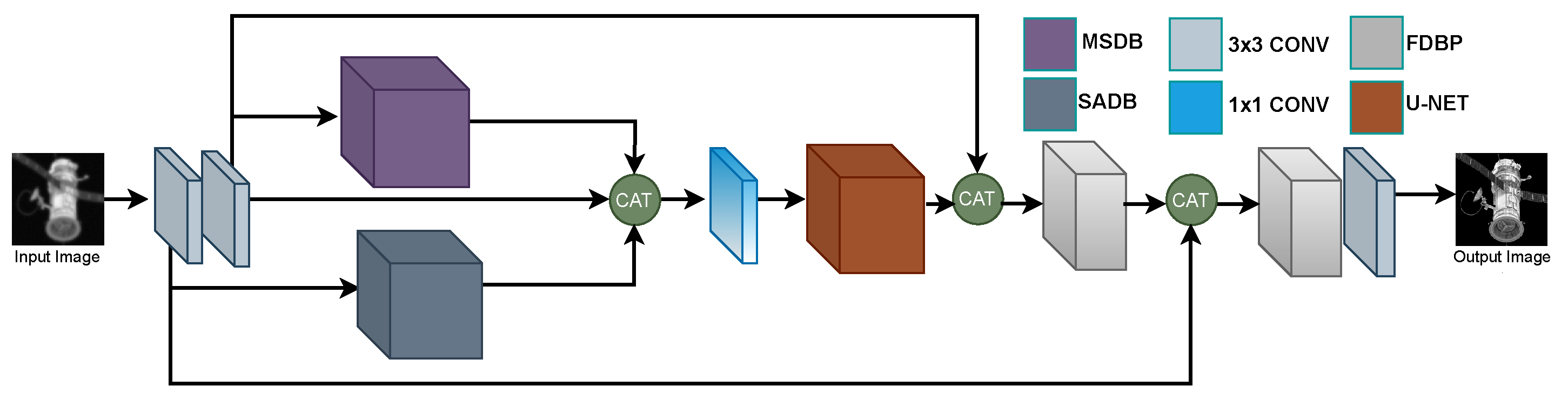
3.2. Proposed Network Model

Instead of trying to express the reconstruction of blur-degraded images as an analytical expression, we design a network model for turbulence-degraded image reconstruction based on the fact that the degradation of multi-factor coupling is inseparable, as shown in Figure 1. The main components of the proposed model include a Multi-Scale Denoising Block (MSDB), a Self-Attention Dense connection Block (SADB) for suppressing noise and preserving more detailed information, and an attention-based asymmetric U-NET module. In this way, the intrinsic features of the image can be extracted from the coupled degraded image by the model, and the image can be reconstructed using these intrinsic features. Further, two FDBPs are used to fuse these intrinsic features and reconstruct sharp images. The proposed restoration reconstruction model can be expressed as:

$$\widehat{f}=F_2(F_1(R(S_M\left(f_p\right)\oplus S_A\left(f_p\right)\oplus f_p)+f_p)+f_p)$$

(5)

Here, $\widehat{f}$ is the reconstructed sharp image, $f_p$ represents the result of the front-end preprocessing of the input-degraded image, $S_M(·)$ represents MSDB, $S_A(·)$ represents SADB, $R(·)$ is for AU-NET, and $F(·)$ is for FDBP. The proposed model first performs shallow feature extraction and denoising on the input image, and then the fused features are used as the input of U-Net. To ensure the reconstructed image has the same information distribution as the original one, this paper uses long skip connections to pass shallow features to the refined reconstruction layer. Thus, the entire model is still an E2E deep convolutional neural network. To make MSDB and SADB in the model mainly focus on removing image noise while the rest of the modules focus on image deblurring, a curriculum learning strategy from local-to-global learning is introduced. For details, see Section 3.3.

3.2.1. MSDB

The main task of this module is to achieve noise suppression by extracting multi-degree features from noisy images and reconstructing noise-free image features. As shown in Figure 2, the encoder of MSDB consists of two multi-scale convolutional layers, each of which consists of three-scale convolutions with kernels of $3\times 3$, $5\times 5$, and $7\times 7$, respectively. The extracted multi-scale features are connected and then passed through a dimensionality reduction fusion layer with a convolution kernel of $1\times 1$ to obtain the high-level features of the degraded image. The decoder of MSDB consists of four dilated convolutional layers, and each dilated convolution is followed by ReLU activation and batch normalization. Dilated convolution has shown good performance in image denoising [62] because it is more beneficial to use contextual information to reconstruct sharp images, and it can increase the receptive field while avoiding the loss of downsampling information. The scale factors of the four dilated convolutional layers of MSDB are 1, 2, 2, and 1, respectively.

3.2.2. SADB

The idea of non-local was used in image denoising in BM3D [47] with remarkable success. To this day, the latest state-of-the-art methods still use non-local as a basic strategy [37,51]. The randomness of noise makes it easier to achieve noise removal by collaborative filtering of correlated regions. In our designed SADB, the self-attention mechanism [63,64] is introduced to realize non-locality. As shown in Figure 3, given an input tensor $X=(H,W,C)$, two 1 × 1 convolutions in parallel are used to change its shape to $(HW,C)$ and $(C,HW)$. Then, multiply these two matrices to get the $(HW,HW)$ matrix and use the softmax activation to get the weighted $(HW,HW)$ matrix. Then, multiply the feature $(C,HW)$ matrix with the weighted $(HW,HW)$ matrix to get the $(C,HW)$ matrix. After changing its shape to $(H,W,C)$, it is added to the initial feature map, and finally, the feature map with weight redistribution is obtained. Non-local attention can be expressed as:

$${\widehat{x}}_i=w\mathrm{softmax}(<w{x}_i·w{x}_j>)\left(w{x}_i\right)+x_i$$

(6)

where x is the input feature, $\widehat{x}$ is the feature after non-local attention processing, and <·> represents the inner product; $wx$ represents a one-dimensional linear embedding, implemented in this work by a convolution of $1\times 1$.

Almost all denoising methods are based on the prior assumption that noise is high-frequency and sparse. Therefore, these algorithms tend to blur the image while removing noise. In the proposed SADB, the dense connection is adopted to solve this problem. SADB takes the weighted feature map as an input and passes it to each subsequent convolutional layer in turn, and dense transmission is also performed between the convolutional layers. This allows the feature map information to flow efficiently, which not only avoids the vanishing gradient but also reduces the depth of the network and allows the network to converge faster. The proposed SADB can better utilize the context information of each layer and retain more image details while removing noise.

3.2.3. AU-NET

Noise-suppressed feature maps are obtained after MSDB and SADB. To further extract effective features from degraded images and reconstruct a sharp image, an attention-based asymmetric U-Net is designed. It uses dilated convolution and batch normalization techniques in the first two layers of encoders to further suppress high-frequency noise in feature maps. Further, under the constraint of the loss function, the encoder has greater modeling ability, which means that its encoding efficiency is higher, and the encoded features are beneficial to the output of the decoder. Further, we use a channel attention mechanism to assign weights to the outputs of the encoder and decoder so that the features of the outputs are more beneficial to the subsequent reconstruction work.

To reduce the information loss caused by fixed downsampling and upsampling, a convolution with stride two is used for downsampling, and a transposed convolution is used for upsampling. Compared with the widely used pooling and interpolation, convolution not only achieves the same downsampling and upsampling effect but also makes the whole process learnable, especially when using the backpropagation algorithm to learn more accurate parameters. Furthermore, the corresponding encoders and decoders are connected by skipping to make the information flow better from shallow layers to deep layers, avoiding a vanishing gradient. Due to the use of noise-reduction processing in the encoding stage and the channel attention mechanism used at the end of encoding and decoding, the entire structure is no longer symmetric, so it is called an attention-based asymmetric U-Net, as shown in Figure 4.

3.2.4. FDBP

The reconstruction of AU-Net is based on high-level features, and there is a potential risk of insufficient reconstruction of detailed texture information. To enhance the presentation ability of the network and restore clearer images, an FDBP is designed. Back-projection has been successfully applied in image super-resolution tasks [39], where it has been shown to have good reconstruction capabilities for texture details. Inspired by it, we design FDBP, which projects high-resolution features into low-resolution space through a downsampling unit, then projects low-resolution features into high-resolution space through an upsampling module, and finally guides network learning by the error between the old and new high-resolution features. The main operations in our designed FDBP are defined as:

$$upsample:x_l=(x_{l-1}\ast k_l){\uparrow }_s,$$

(7)

$$downsample:x_l=(x_{l-1}\ast k_l){\downarrow }_s,$$

(8)

$$residual:e_l=x_1-x_{l-1},$$

(9)

$$upresidualsample:x_l=(x_{l-1}\ast k_l){\uparrow }_s,$$

(10)

$$output:x_l=x_0+x_l,$$

(11)

where $x_0$ represents the feature after convolution of the input, and $x\ast k$ is the convolution of $3\times 3$. To enhance the flow of information and keep the reconstructed features consistent, we use two FDBP operations. The FDBP module we designed is shown in Figure 5 and can capture multi-scale context information well and downsample the feature map to a small space to save memory and speed up network training.

3.3. Curriculum Learning Strategy

Due to the randomness of various types of noise, the spatial dimension of the samples of multi-factor-coupled degraded images is very large, and its representation learning is very difficult. Therefore, a complex neural network needs to be designed to achieve its restoration. In such cases, due to the complexity of the problem and the scale of the parameters, the learning difficulty of the neural network is increased. Curriculum learning [65,66,67] is considered an effective way to address this problem. Aiming at the difficulty of multi-factor-coupled image restoration, a systematic curriculum learning strategy from local-to-global network and from easy-to-difficult data learning is designed.

3.3.1. Local-to-Global Network Learning

Multi-task decomposition is helpful to reduce the difficulty of the restoration of multi-factor-coupled images. Although the restoration of turbulence-degraded images is difficult to simply decompose into multiple independent tasks [60], we design the NSTR neural network based on the weak assumption that images are mainly affected by additive noise and turbulence blur. Since MSDB and SADB are primarily good at noise suppression, these two modules are trained separately. First, a new training set is constructed by adding Gaussian noise and Poisson noise to the blurred images, and the blurred images without noise are used as labels. Then, the output components are plugged into MSDB and SADB, respectively. Finally, MSDB and SADB are pre-trained to obtain weight parameters.

After completing the training of MSDB and SADB, their weights are transferred to the overall network model. This transfer learning strategy enables NSRN to have a certain ability to suppress noise from the beginning. To preserve the noise suppression ability of MSDB and SADB in the overall training of NSRN, the learning rate should be set to a small value. In our experiments, the overall learning rate is set to 0.1. By fine-tuning the learning rate, the proposed network not only maintains noise suppression effectively but also focuses a lot of attention on image deconvolution reconstruction. This kind of curriculum learning strategy of first local and then global features not only reduces the learning difficulty of the whole model but also avoids strict task decomposition.

3.3.2. Easy-to-Difficult Data Curriculum Learning

The main reason for the difficulty in restoring turbulence-blurred images is the high dynamics of turbulent flow, which results in a large spatial distribution of samples. We find it extremely difficult to train the network directly with severely turbulence-degraded images. Therefore, the easy-to-difficult learning strategy is used to train the NSRN network. By setting the value of the atmospheric coherence length r, data with different degrees of blur can be obtained. In this paper, three r values are used to obtain data with mild, moderate, and severe blur, respectively. First, initial network training is performed via the weight initialization method provided by He [68], and then the network is sequentially trained using datasets with varying degrees of blur from mild to severe. After the mild set converges, its weights are saved and used for weight initialization for training on the blurrier datasets. Through this easy-to-difficult training strategy, the proposed network can eventually learn more complex mappings and achieve better results.

NSRN uses the $L1$ loss function for training. The inputs to train the local modules MSDB and SADB are noisy blurred images, and the labels are blurred images without noise. The input to train the entire model is degraded images, and the labels are sharp images. The loss function in the network can be formulated as:

$$L\left(\mathsf{\Theta }\right)=\frac{1}{N}\sum _{i=1}^N{∥\widehat{y}-y∥}_1,$$

(12)

where ${∥·∥}_1$ can restore better texture information. PyTorch was used to implement the proposed network model, and the whole network was trained using GTX 1080Ti under Ubuntu 16. The image block size used for training is $32\times 32$, and the default setting for the batch size is 64. Since the input and output images of the network have the same resolution, any image resolution can be used in testing. To make the network converge faster, a learning-rate decay strategy is used; that is, the initial learning rate is set to 0.001 and decays to 0.5 times the previous learning rate every 50 epochs. Overall training used 250 epochs. A Mean Squared Error loss function (MSE) is used, and the Adam optimizer is used to constrain gradient descent. The learning algorithm of the proposed NSRN is shown in Algorithm 1. The experimental convergence curve of Algorithm 1 is shown in Figure 6. The restoration of mildly degraded images is less difficult, and the model converges well. As shown in Figure 6a, both training accuracy and validation accuracy converge to better positions. Both moderate degradation and severe degradation converge to low error levels due to the curriculum learning strategy (see Figure 6b,c). In moderate degradation, the validation curve indicates slight overfitting. In severe degradation, the validation curve indicates oscillation at the beginning and convergence after 125 epochs. The training time is 8.5 min/per epoch. When the test image size is 384 × 384 pixels, the inference time is 0.24 s/frame.

Algorithm 1 Systematic curriculum learning algorithm for NSRN
Require:
		B: number of MSDB and SADB training;
		$D=\{D_1,D_2,D_n\}$: NSRN training set;
		$w_0$: weight initialization.
Ensure:
		NSRN(w): parameters of NSRN.
	1:	Begin:
		/* local-to-global learning */
	2:	MSDB learning: $s_m\left(w_s\right)=S_m\left(f_p\left(B\right)\right)$, where $w_s$ is the parameter of MSDB
	3:	SADB learning: $s_A\left(w_A\right)=S_A\left(f_p\left(B\right)\right)$, where $w_A$ is the parameter of SADB
		/* easy-to-difficult learning */
	4:	Initialize MSDB in NSRN with $w_s$
	5:	Initialize SADB in NSRN with $w_A$
	6:	for each $D_i$ do
	7:	NSRN learning: NSRN $\left(w_i\right)=F_2(F_1(R(S_M\left(f_p\right)\oplus S_A\left(f_p\right)\oplus f_p)+f_p)+f_p)$
	8:	end for
	9:	Initialize NSRN with $w_n$
	10:	Train NSRN with all training data D
	11:	Output: NSRN

4. Experiments and Discussions

4.1. Dataset

There are few public real-space target images, and ground-truth labels of degraded images are also difficult to obtain. Therefore, degraded image simulation is used to obtain training data to verify the effectiveness of the proposed method. The 3D models used to obtain images of simulated space objects are from STK (Satellite Tool Kit) [69], which provides various satellite models and turbulence degradation models. The reflected sunlight of space objects is refracted by atmospheric turbulence, which makes the images observed by ground-based telescopes blurred. This turbulence blur can be represented by the following model [28].

$$h(u,v)=e^{\{-3.44{\left(\frac{\lambda fU}{r}\right)}^{5/3}\}}$$

(13)

where $U=\sqrt{u^2+v^2}$ is the frequency, $(u,v)$ is the unit pulse, $\lambda$ is the wavelength, f is the optical focal length, and r is the atmosphere coherence length. It can be seen that the larger the r, the stronger the atmospheric motion and the blurrier the image. Therefore, different degrees of turbulence blurred images can be generated by changing the size of r.

To obtain more diverse training data, clear satellite images with different attitude angles are obtained by rotating the 3D satellite model from STK. The acquired images are data-enhanced, including rotating 90, 180, and 270 degrees and flipping horizontally and vertically. Images are then blurred using the atmospheric turbulence long-exposure degradation function shown in Equation (13). By setting different r values in [0, 0.02], blurred image datasets with three levels contained in three subsets—mildly degraded (r ∈ [0.005, 0.01)), moderately degraded (r ∈ [0.005, 0.015)), and severely degraded (r ∈ [0.005, 0.02])—can be obtained. During atmospheric turbulence imaging, the turbulence blurring is also mixed with photon noise, dark noise, reset noise, and readout noise. These noises mainly obey Gaussian and Poisson distributions, so we add Gaussian noise and Poisson noise to the blurred image. The value range of the parameter of Gaussian noise is [35, 42], and the value range of the parameter of Poisson noise is [4, 7]. The real degradation model is expressed as:

$$f(x,y)=g(x,y)\ast h(x,y)+n(x,y)+p(x,y),$$

(14)

where f is the observed image, g is the original image, h is the PSF atmospheric turbulence, n represents Gaussian noise, and p represents Poisson noise. To ensure the generalization ability of the model and encourage the restoration model to learn the blur degradation mode and the corresponding restoration mode, we adopt the strategy of training on small images and verifying and testing on large images.

We cut the image at 20-pixel intervals to generate $32\times 32$ image patches and then discarded samples in which more than 90% of the patches were black background area, resulting in 117,300 image patches for training the model. Some of the generated training samples are shown in Figure 7. A total of 56 large images that are not used to for the training set are used as the test set, and some test samples are shown in Figure 8. We also collected 17 real-world turbulence-degraded images from public sources as a test set, as shown in Figure 9. Detailed information about the dataset is show in

Table 1. Composition details of dataset.

		Number of Large Images	Number of Image Patches
Training set	mild	1358	117,300
	moderate	1358	117,300
	severe	1358	117,300
Validation set	mild	100	/
	moderate	100	/
	severe	100	/
Simulated test set	mild	56	/
	moderate	56	/
	severe	56	/
Real test set	/	17	/

. The spatial resolutions of the large images in the table are not uniform, and their ranges is [256 × 256, 1024 × 1024].

4.2. Metrics for Evaluation and Methods for Comparison

The simulated images have labels, so the performance evaluation of the algorithm can be carried out by combining subjective methods and objective metrics. For objective metrics, peak signal-to-noise ratio (PSNR) and structural similarity (SSIM) are used to evaluate the restoration performance of each algorithm. For subjective metrics, the quality of the restored image is evaluated by human vision and the reference images. Moreover, for real images, due to the lack of reference images, only subjective evaluation and no-reference metrics can be used. In this paper, the no-reference evaluation metrics used are Brenner, Laplacian, SMD, Variance, Energy, Vollath, and Entropy. The calculation methods of these no-reference metrics can be found in [70].

Gao [2] conducted extensive analysis on traditional restoration methods for spatial images. The experimental results show that the traditional methods are not ideal for removing turbulence blur, so the proposed method is not compared using traditional methods. To better analyze and evaluate the performance of this method, some representative deep learning methods are selected for comparative experiments, namely Gao [2], Chen [38], Mao-30 [49], MemNet [50], CBDNet [48], ADNet [31], DPDNN [53], and DPIR [36]. For absolute fairness, for all comparison methods, we use the parameters given in the original text and train them with the training set of this paper.

4.3. Ablation Experiment

Our proposed model (Figure 1) uses an asymmetric U-NET as the backbone. To verify the effectiveness of the proposed model, an ablation experiment is performed. In this experiment, the backbone U-NET is named Model1, and Model1 to Model6 are formed by plugging MSDB, SADB, FDBP, and curriculum learning strategy (TNRS) into Model1, as shown in

Table 2. Performance of models with different components (The best results are shown in bold fonts).

		Model1	Model2	Model3	Model4	Model5	Model6
U-Net		√	√	√	√	√	√
MSDB			√		√	√	√
SADB				√	√	√	√
FDBP						√	√
TNRS							√
PSNR	mild	29.2092	29.8803	29.8666	30.0160	30.0587	30.1817
	moderate	27.9264	28.2895	28.0992	28.2989	28.3944	28.6400
	severe	25.9631	27.2224	27.1046	27.6352	27.8129	28.0169
SSIM	mild	0.8889	0.8923	0.8869	0.9001	0.8911	0.9035
	moderate	0.8430	0.8649	0.8757	0.8685	0.8701	0.8732
	severe	0.7052	0.8363	0.8218	0.8325	0.8341	0.8545

. When training models Model1–Model5, three training subsets with different blur degrees are directly merged as the final training set. Model6 is trained using the steps shown in Algorithm 1. The trained model is tested on three different degraded images; the results of the objective evaluation metric are shown in Table 2, and the partially restored images are shown in Figure 10.

It can be seen from Table 2 that: (1) Model1, which only contains the backbone U-NET, lacked sufficient representation power to learn intrinsic features from degraded images and reconstruct images well. (2) The PSNR of Model2 obtained by plugging MSDB into Model1 was significantly improved because MSDB enables U-NET to have better global and local information presentation capabilities. However, the PSNR of Model3 obtained by plugging SADB into Model1 decreased, but the image details are richer. (3) Model4 was obtained by plugging MSDB and SADB into Model1. Compared with Model1, Model2, and Model3, both the PSNR and the SSIM significantly improved in Model4. This is because Model4 has stronger noise suppression performance. (4) Model5, obtained by plugging FBPR into Model4, obtained more consistent results. (5) Model6 (NSRN) added the curriculum learning algorithm to Model5 to train the network. The performance of Model6 was further improved compared to Model5, which proves that the proposed model does have better generalization ability, and it is easier to capture the mapping relationship between sharp images and low-resolution images. Moreover, from the restored images of each model in Figure 10, the results of Model 6 have the best visual effect, and the edges and textures are clearer.

4.4. Experiments and Comparative Analysis of Simulated Images

(1)

Model for mild degradation

We use the trained model for restoration experiments on test data with mild degradation, and the resulting averages of objective evaluation metrics are shown in

Table 3. Average PSNR and SSIM of different state-of-the-art methods on mild degradation (The best results are shown in bold fonts).

Methods	PSNR	SSIM
Gao	27.5423	0.8337
Chen	28.0156	0.8431
Mao	29.3903	0.8387
MemNet	27.8413	0.8295
CBDNet	29.4395	0.8596
ADNet	29.7430	0.8828
DPDNN	30.0122	0.8999
DPIR	29.7316	0.8932
Ours	30.1817	0.9035

. It can be seen that for PSNR, Mao, CBDNet, ADNet, DPDNN, DPIR, and the proposed method all achieve very good results. These methods all have more complex network models, so they have better presentation ability. For SSIM, DPDNN, DPIR, and our method have significantly better performance than the remaining methods, which shows that the method based on noise suppression has a better ability to restore textual details. Compared to the second-ranked method, our method improves PSNR by 0.16 and improves SSIM by 0.036. An example set of restored results is shown in Figure 11. It can be seen that for mildly degraded images, almost all methods achieve better visual effects.

(2)

Model for moderate degradation

The test results of all models on the moderately degraded dataset are shown in

Table 4. Average PSNR and SSIM of different state-of-the-art methods on moderate degradation (The best results are shown in bold fonts).

Methods	PSNR	SSIM
Gao	25.8558	0.7643
Chen	26.9923	0.8297
Mao	28.3321	0.8446
MemNet	26.4702	0.7480
CBDNet	27.7382	0.7817
ADNet	28.1007	0.8472
DPDNN	28.3600	0.8766
DPIR	28.3519	0.8284
Ours	28.6400	0.8732

. It can be seen that for PSNR, DPIR, DPDNN, and Mao achieve competitive results. However, our method has the best performance and is nearly 0.3 higher than the second-ranked method, indicating that the proposed method does have a strong representation of learning ability by introducing modules such as FBPR. On SSIM, the best method is DPDNN, and our method is close to DPDNN. The restoration results of different methods on a typical moderately degraded image are shown in Figure 12. It can be seen that the visual effects of images restored by DPDNN, DPIR, Mao, and our method are similar. However, in contrast, DPDNN has sharper edges in some regions, and our method is more consistent.

(3)

Model for severe degradation

The results of objective evaluation metrics of all restoration models on the severely degraded image test set are shown in

Table 5. Average PSNR and SSIM of different state-of-the-art methods on severe degradation (The best results are shown in bold fonts).

Methods	PSNR	SSIM
Gao	26.7512	0.7934
Chen	27.1416	0.8250
Mao	27.1224	0.8190
MemNet	26.1868	0.7288
CBDNet	27.4253	0.8471
ADNet	27.1676	0.8346
DPDNN	27.8129	0.8431
DPIR	27.6249	0.8376
Ours	28.0169	0.8545

. It can be seen that our method has obvious advantages in this dataset: the PSNR is higher than the second-ranked method by nearly 0.2, and the SSIM is higher than the second-ranked method by 0.007. Further, for PSNR, our method is the only one that exceeds 28. Our method is also the only method that shows the best performance in both metrics, which shows that for severely degraded images with severe noise and severe blur, the method that can specifically deal with the noise is more competitive. The restoration results of different methods on a typical severely degraded image are shown in Figure 13. From the visual effect, our method restores more texture details and has obvious advantages.

In general, the proposed method, DPDNN, and DPIR are the most competitive methods, while the Gao, Mao, and Chen models are too small to represent the huge sample space spanned by severely degraded images. This shows that a network that can restore heavily noisy and blurred severely degraded images not only needs sufficient representation ability but also some mechanism for learning features, such as attention. Moreover, as the model becomes more complex, the generalization ability and restoration ability of the network model can be improved by separately processing blur and noise.

To better compare the performance of each algorithm under different noise levels, an image is randomly selected from the test set and then mixed with different levels of noise for restoration experiments. As seen in Figure 14, DPIR and our method have similar performance on SSIM. DPDNN also has good performance when the noise intensity is greater than 35. Moreover, our method has the best PSNR at almost all noise levels.

4.5. Experiments and Comparative Analysis of Real Images

The results of the non-reference evaluation metrics of the restoration results obtained by all the compared methods on real data are shown in

Table 6. Results of non-reference evaluation metrics on real test data (The best results are shown in bold fonts).

Method	Brenner (xe6)	Laplacian	SMD (xe4)	Variance (xe7)	Energy (xe6)	Vollath (xe7)	Entropy
ADNet	27.36	346.52	53.9847	17.477	19.42	17.05	2.58
CBDNet	23.07	310.00	49.80	17.42	16.85	17.06	2.51
Chen	27.62	419.92	56.31	17.57	19.92	17.13	2.68
Gao	24.45	231.94	52.34	17.41	16.53	17.05	2.61
Mao	16.71	220.832	43.61	16.83	12.48	16.58	2.32
MemNet	21.23	314.55	48.71	16.41	15.96	16.08	2.52
Zhang	19.26	242.84	46.14	17.85	13.90	17.55	2.49
DPDNN	15.65	183.75	42.31	16.31	11.29	16.07	2.57
Ours	32.54	493.77	58.98	18.13	23.47	17.61	2.41

, and the restoration results on real data are shown in Figure 15. There was still a big difference between the simulated training data and the real image distribution, and all methods encountered cross-domain problems. However, under the same conditions, our method is the best in these numerical experiments and these evaluation metrics. Of course, the reliability of the no-reference evaluation and the consistency with human vision require further research [24]. The proposed method has a certain enhancement of texture and edges, so metrics such as upper edge and gradient have weak advantages over other methods. As shown in Figure 15, due to the weak network representation ability of the methods of Gao [2] and Mao [49], the restored image is still blurred. The rest of the methods can provide visually pleasing restoration. The visual effect restored by the method of Chen [38] is close to our method, indicating that our method has excellent performance for the restoration of severely degraded images. This is because it treated additive noise and blur degradation separately and designed special modules to denoise and perform blur deconvolution.

5. Conclusions

Atmospheric turbulence-blurred images are usually observed at long distances and contain severe noise. Therefore, the restoration of atmospheric turbulence-degraded images includes two tasks: deblurring and denoising. Although deblurring and denoising belong to the same underlying visual tasks, their internal principles are different. Denoising removes high-frequency noise in images, while deblurring using deconvolution to obtain high-frequency information from blurred images. Based on this knowledge, we design a deep neural network model for the restoration of atmospheric turbulence-degraded images based on curriculum learning. Noise suppression of degraded images is achieved by designing a dedicated denoiser without enforcing fully decoupled denoising and deblurring. The experimental results demonstrate the effectiveness of our method. However, the restoration of real turbulence-degraded images is still an open problem. The design of a GAN [71] model based on the ideas proposed in this paper to improve the restoration of real images will be the direction and focus of future research.

References

1. Jefferies, S.M.; Hart, M. Deconvolution from wave front sensing using the frozen flow hypothesis. Opt. Express 2011, 19, 1975–1984. [Google Scholar] [CrossRef] [PubMed]
2. Gao, Z.; Shen, C.; Xie, C. Stacked convolutional auto-encoders for single space target image blind deconvolution. Neurocomputing 2018, 313, 295–305. [Google Scholar] [CrossRef]
3. Mourya, R.; Denis, L.; Becker, J.M.; Thiébaut, E. A blind deblurring and image decomposition approach for astronomical image restoration. In Proceedings of the 2015 23rd European Signal Processing Conference (EUSIPCO), Nice, France, 31 August–4 September 2015; IEEE: New York, NY, USA, 2015; pp. 1636–1640. [Google Scholar]
4. Yan, L.; Jin, M.; Fang, H.; Liu, H.; Zhang, T. Atmospheric-turbulence-degraded astronomical image restoration by minimizing second-order central moment. IEEE Geosci. Remote Sens. Lett. 2012, 9, 672–676. [Google Scholar]
5. Zhu, X.; Milanfar, P. Removing atmospheric turbulence via space-invariant deconvolution. IEEE Trans. Pattern Anal. Mach. Intell. 2012, 35, 157–170. [Google Scholar] [CrossRef]
6. Xie, Y.; Zhang, W.; Tao, D.; Hu, W.; Qu, Y.; Wang, H. Removing turbulence effect via hybrid total variation and deformation-guided kernel regression. IEEE Trans. Image Process. 2016, 25, 4943–4958. [Google Scholar] [CrossRef]
7. Gilles, J.; Dagobert, T.; De Franchis, C. Atmospheric Turbulence Restoration by Diffeomorphic Image Registration and Blind Deconvolution. In Advanced Concepts for Intelligent Vision Systems; Springer: Berlin/Heidelberg, Germany, 2008; pp. 400–409. [Google Scholar]
8. Jin, M.; Meishvili, G.; Favaro, P. Learning to extract a video sequence from a single motion-blurred image. In Proceedings of the IEEE Conference on Computer Vision and Pattern Recognition, Salt Lake City, UT, USA, 18–22 June 2018; pp. 6334–6342. [Google Scholar]
9. Xu, X.; Pan, J.; Zhang, Y.J.; Yang, M.H. Motion blur kernel estimation via deep learning. IEEE Trans. Image Process. 2017, 27, 194–205. [Google Scholar] [CrossRef]
10. Zhou, C.; Lin, S.; Nayar, S.K. Coded aperture pairs for depth from defocus and defocus deblurring. Int. J. Comput. Vis. 2011, 93, 53–72. [Google Scholar] [CrossRef]
11. Vasu, S.; Maligireddy, V.R.; Rajagopalan, A. Non-blind deblurring: Handling kernel uncertainty with cnns. In Proceedings of the IEEE Conference on Computer Vision and Pattern Recognition, Salt Lake City, UT, USA, 18–23 June 2018; pp. 3272–3281. [Google Scholar]
12. Zhang, J.; Pan, J.; Lai, W.S.; Lau, R.W.; Yang, M.H. Learning fully convolutional networks for iterative non-blind deconvolution. In Proceedings of the IEEE Conference on Computer Vision and Pattern Recognition, Honolulu, HI, USA, 21–26 July 2017; pp. 3817–3825. [Google Scholar]
13. Schuler, C.J.; Hirsch, M.; Harmeling, S.; Schölkopf, B. Learning to deblur. IEEE Trans. Pattern Anal. Mach. Intell. 2015, 38, 1439–1451. [Google Scholar] [CrossRef]
14. Zhang, Y.; Lau, Y.; Kuo, H.w.; Cheung, S.; Pasupathy, A.; Wright, J. On the global geometry of sphere-constrained sparse blind deconvolution. In Proceedings of the IEEE Conference on Computer Vision and Pattern Recognition, Honolulu, HI, USA, 21–26 July 2017; pp. 4894–4902. [Google Scholar]
15. Dai, C.; Lin, M.; Wu, X.; Zhang, D. Single hazy image restoration using robust atmospheric scattering model. Signal Process. 2020, 166, 107257. [Google Scholar] [CrossRef]
16. Hu, D.; Tan, J.; Zhang, L.; Ge, X.; Liu, J. Image deblurring via enhanced local maximum intensity prior. Signal Process. Image Commun. 2021, 96, 116311. [Google Scholar] [CrossRef]
17. Zhang, H.; Wipf, D.; Zhang, Y. Multi-image blind deblurring using a coupled adaptive sparse prior. In Proceedings of the IEEE Conference on Computer Vision and Pattern Recognition, Portland, OR, USA, 23–28 June 2013; pp. 1051–1058. [Google Scholar]
18. Xu, L.; Zheng, S.; Jia, J. Unnatural l0 sparse representation for natural image deblurring. In Proceedings of the IEEE Conference on Computer Vision and Pattern Recognition, Portland, OR, USA, 23–28 June 2013; pp. 1107–1114. [Google Scholar]
19. Rostami, M.; Michailovich, O.; Wang, Z. Image Deblurring Using Derivative Compressed Sensing for Optical Imaging Application. IEEE Trans. Image Process. 2012, 21, 3139–3149. [Google Scholar] [CrossRef] [PubMed] [Green Version]
20. He, R.; Wang, Z.; Fan, Y.; Fengg, D. Atmospheric turbulence mitigation based on turbulence extraction. In Proceedings of the 2016 IEEE International Conference on Acoustics, Speech and Signal Processing (ICASSP), Shanghai, China, 20–25 March 2016; pp. 1442–1446. [Google Scholar] [CrossRef]
21. Li, D.; Mersereau, R.M.; Simske, S. Atmospheric Turbulence-Degraded Image Restoration Using Principal Components Analysis. IEEE Geosci. Remote Sens. Lett. 2007, 4, 340–344. [Google Scholar] [CrossRef]
22. Krishnan, D.; Fergus, R. Fast image deconvolution using hyper-Laplacian priors. Adv. Neural Inf. Process. Syst. 2009, 22, 1033–1041. [Google Scholar]
23. Perrone, D.; Favaro, P. Total variation blind deconvolution: The devil is in the details. In Proceedings of the IEEE Conference on Computer Vision and Pattern Recognition, Columbus, OH, USA, 23–28 June 2014; pp. 2909–2916. [Google Scholar]
24. Pan, J.; Hu, Z.; Su, Z.; Yang, M.H. Deblurring text images via L0-regularized intensity and gradient prior. In Proceedings of the IEEE Conference on Computer Vision and Pattern Recognition, Columbus, OH, USA, 23–28 June 2014; pp. 2901–2908. [Google Scholar]
25. Mou, C.; Zhang, J. Graph Attention Neural Network for Image Restoration. In Proceedings of the 2021 IEEE International Conference on Multimedia and Expo (ICME), Taipei, Taiwan, 18–22 July 2022; IEEE: New York, NY, USA, 2021; pp. 1–6. [Google Scholar]
26. Anwar, S.; Barnes, N.; Petersson, L. Attention-Based Real Image Restoration. IEEE Trans. Neural Netw. Learn. Syst. 2021, 1–11. [Google Scholar] [CrossRef] [PubMed]
27. Yu, K.; Wang, X.; Dong, C.; Tang, X.; Loy, C.C. Path-restore: Learning network path selection for image restoration. IEEE Trans. Pattern Anal. Mach. Intell. 2021, 44, 7078–7092. [Google Scholar] [CrossRef]
28. Chen, G.; Gao, Z.; Wang, Q.; Luo, Q. U-net like deep autoencoders for deblurring atmospheric turbulence. J. Electron. Imaging 2019, 28, 053024. [Google Scholar] [CrossRef]
29. Liu, B.; Shu, X.; Wu, X. Demoiréing of Camera-Captured Screen Images Using Deep Convolutional Neural Network. arXiv 2018, arXiv:1804.03809. [Google Scholar]
30. Zhang, K.; Zuo, W.; Chen, Y.; Meng, D.; Zhang, L. Beyond a gaussian denoiser: Residual learning of deep cnn for image denoising. IEEE Trans. Image Process. 2017, 26, 3142–3155. [Google Scholar] [CrossRef] [PubMed]
31. Tian, C.; Xu, Y.; Li, Z.; Zuo, W.; Fei, L.; Liu, H. Attention-guided CNN for image denoising. Neural Netw. 2020, 124, 117–129. [Google Scholar] [CrossRef]
32. Retraint, F.; Zitzmann, C. Quality factor estimation of jpeg images using a statistical model. Digit. Signal Process. 2020, 103, 102759. [Google Scholar] [CrossRef]
33. Sim, H.; Kim, M. A deep motion deblurring network based on per-pixel adaptive kernels with residual down-up and up-down modules. In Proceedings of the IEEE/CVF Conference on Computer Vision and Pattern Recognition Workshops, Long Beach, CA, USA, 16–20 June 2019. [Google Scholar]
34. Zhang, H.; Dai, Y.; Li, H.; Koniusz, P. Deep stacked hierarchical multi-patch network for image deblurring. In Proceedings of the IEEE/CVF Conference on Computer Vision and Pattern Recognition, Long Beach, CA, USA, 16–20 June 2019; pp. 5978–5986. [Google Scholar]
35. Mao, Z.; Chimitt, N.; Chan, S.H. Accelerating Atmospheric Turbulence Simulation via Learned Phase-to-Space Transform. In Proceedings of the IEEE/CVF International Conference on Computer Vision, Montreal, QC, Canada, 10–17 October 2021; pp. 14759–14768. [Google Scholar]
36. Zhang, K.; Li, Y.; Zuo, W.; Zhang, L.; Van Gool, L.; Timofte, R. Plug-and-play image restoration with deep denoiser prior. IEEE Trans. Pattern Anal. Mach. Intell. 2021, 44, 6360–6376. [Google Scholar] [CrossRef]
37. Zhang, K.; Zuo, W.; Gu, S.; Zhang, L. Learning deep CNN denoiser prior for image restoration. In Proceedings of the IEEE Conference on Computer Vision and Pattern Recognition, Honolulu, HI, USA, 21–26 July 2017; pp. 3929–3938. [Google Scholar]
38. Chen, G.; Gao, Z.; Wang, Q.; Luo, Q. Blind de-convolution of images degraded by atmospheric turbulence. Appl. Soft Comput. 2020, 89, 106131. [Google Scholar] [CrossRef]
39. Haris, M.; Shakhnarovich, G.; Ukita, N. Deep back-projection networks for super-resolution. In Proceedings of the IEEE Conference on Computer Vision and Pattern Recognition, Salt Lake City, UT, USA, 18–23 June 2018; pp. 1664–1673. [Google Scholar]
40. Chatterjee, M.R.; Mohamed, A.; Almehmadi, F.S. Secure free-space communication, turbulence mitigation, and other applications using acousto-optic chaos. Appl. Opt. 2018, 57, C1–C13. [Google Scholar] [CrossRef] [PubMed]
41. Ramos, A.A.; de la Cruz Rodríguez, J.; Yabar, A.P. Real-time, multiframe, blind deconvolution of solar images. Astron. Astrophys. 2018, 620, A73. [Google Scholar] [CrossRef]
42. Zha, Z.; Wen, B.; Yuan, X.; Zhou, J.; Zhu, C. Image restoration via reconciliation of group sparsity and low-rank models. IEEE Trans. Image Process. 2021, 30, 5223–5238. [Google Scholar] [CrossRef]
43. Zha, Z.; Yuan, X.; Zhou, J.; Zhu, C.; Wen, B. Image restoration via simultaneous nonlocal self-similarity priors. IEEE Trans. Image Process. 2020, 29, 8561–8576. [Google Scholar] [CrossRef] [PubMed]
44. Venkatakrishnan, S.V.; Bouman, C.A.; Wohlberg, B. Plug-and-play priors for model based reconstruction. In Proceedings of the 2013 IEEE Global Conference on Signal and Information Processing, Austin, TX, USA, 3–5 December 2013; IEEE: New York, NY, USA, 2013; pp. 945–948. [Google Scholar]
45. Wei, K.; Aviles-Rivero, A.; Liang, J.; Fu, Y.; Schönlieb, C.B.; Huang, H. Tuning-free plug-and-play proximal algorithm for inverse imaging problems. In Proceedings of the International Conference on Machine Learning, PMLR, Virtual Event, 13–18 July 2020; pp. 10158–10169. [Google Scholar]
46. Nair, P.; Gavaskar, R.G.; Chaudhury, K.N. Fixed-point and objective convergence of plug-and-play algorithms. IEEE Trans. Comput. Imaging 2021, 7, 337–348. [Google Scholar] [CrossRef]
47. Dabov, K.; Foi, A.; Katkovnik, V.; Egiazarian, K. Image denoising by sparse 3-D transform-domain collaborative filtering. IEEE Trans. Image Process. 2007, 16, 2080–2095. [Google Scholar] [CrossRef]
48. Hradiš, M.; Kotera, J.; Zemcık, P.; Šroubek, F. Convolutional neural networks for direct text deblurring. In Proceedings of the BMVC, Swansea, UK, 7–10 September 2015; Volume 10. [Google Scholar]
49. Mao, X.; Shen, C.; Yang, Y.B. Image restoration using very deep convolutional encoder-decoder networks with symmetric skip connections. Adv. Neural Inf. Process. Syst. 2016, 29, 2810–2818. [Google Scholar]
50. Tai, Y.; Yang, J.; Liu, X.; Xu, C. Memnet: A persistent memory network for image restoration. In Proceedings of the IEEE International Conference on Computer Vision, Venice, Italy, 22–29 October 2017; pp. 4539–4547. [Google Scholar]
51. Song, G.; Sun, Y.; Liu, J.; Wang, Z.; Kamilov, U.S. A new recurrent plug-and-play prior based on the multiple self-similarity network. IEEE Signal Process. Lett. 2020, 27, 451–455. [Google Scholar] [CrossRef]
52. Asim, M.; Shamshad, F.; Ahmed, A. Blind image deconvolution using deep generative priors. IEEE Trans. Comput. Imaging 2020, 6, 1493–1506. [Google Scholar] [CrossRef]
53. Dong, W.; Wang, P.; Yin, W.; Shi, G.; Wu, F.; Lu, X. Denoising prior driven deep neural network for image restoration. IEEE Trans. Pattern Anal. Mach. Intell. 2018, 41, 2305–2318. [Google Scholar] [CrossRef]
54. Sun, Y.; Wu, Z.; Xu, X.; Wohlberg, B.; Kamilov, U.S. Scalable plug-and-play ADMM with convergence guarantees. IEEE Trans. Comput. Imaging 2021, 7, 849–863. [Google Scholar] [CrossRef]
55. Terris, M.; Repetti, A.; Pesquet, J.C.; Wiaux, Y. Enhanced convergent pnp algorithms for image restoration. In Proceedings of the 2021 IEEE International Conference on Image Processing (ICIP), Anchorage, AK, USA, 19–22 September 2021; IEEE: New York, NY, USA, 2021; pp. 1684–1688. [Google Scholar]
56. Gao, S.; Zhuang, X. Rank-One Network: An Effective Framework for Image Restoration. IEEE Trans. Pattern Anal. Mach. Intell. 2020, 44, 3224–3238. [Google Scholar] [CrossRef]
57. Jung, H.; Kim, Y.; Min, D.; Jang, H.; Ha, N.; Sohn, K. Learning Deeply Aggregated Alternating Minimization for General Inverse Problems. IEEE Trans. Image Process. 2020, 29, 8012–8027. [Google Scholar] [CrossRef]
58. Ryu, E.; Liu, J.; Wang, S.; Chen, X.; Wang, Z.; Yin, W. Plug-and-play methods provably converge with properly trained denoisers. In Proceedings of the International Conference on Machine Learning, PMLR, Long Beach, CA, USA, 9–15 June 2019; pp. 5546–5557. [Google Scholar]
59. Geman, D.; Yang, C. Nonlinear image recovery with half-quadratic regularization. IEEE Trans. Image Process. 1995, 4, 932–946. [Google Scholar] [CrossRef]
60. Chen, G.; Gao, Z.; Zhou, B.; Zuo, C. Optimization and regularization of complex task decomposition for blind removal of multi-factor degradation. J. Vis. Commun. Image Represent. 2022, 82, 103384. [Google Scholar] [CrossRef]
61. Wu, J.; Di, X. Integrating neural networks into the blind deblurring framework to compete with the end-to-end learning-based methods. IEEE Trans. Image Process. 2020, 29, 6841–6851. [Google Scholar] [CrossRef]
62. Anwar, S.; Barnes, N. Real image denoising with feature attention. In Proceedings of the IEEE/CVF International Conference on Computer Vision, Seoul, Korea, 27 October–2 November 2019; pp. 3155–3164. [Google Scholar]
63. Zhang, Y.; Li, K.; Li, K.; Zhong, B.; Fu, Y. Residual non-local attention networks for image restoration. arXiv 2019, arXiv:1903.10082. [Google Scholar]
64. He, W.; Yao, Q.; Li, C.; Yokoya, N.; Zhao, Q.; Zhang, H.; Zhang, L. Non-local meets global: An integrated paradigm for hyperspectral image restoration. IEEE Trans. Pattern Anal. Mach. Intell. 2020, 44, 2089–2107. [Google Scholar] [CrossRef]
65. Graves, A.; Bellemare, M.G.; Menick, J.; Munos, R.; Kavukcuoglu, K. Automated curriculum learning for neural networks. In Proceedings of the International Conference on Machine Learning, PMLR, Sydney, Australia, 6–11 August 2017; pp. 1311–1320. [Google Scholar]
66. Jiang, L.; Zhou, Z.; Leung, T.; Li, L.J.; Fei-Fei, L. Mentornet: Learning data-driven curriculum for very deep neural networks on corrupted labels. In Proceedings of the International Conference on Machine Learning, PMLR, Stockholm, Sweden, 10–15 July 2018; pp. 2304–2313. [Google Scholar]
67. Yang, L.; Shen, Y.; Mao, Y.; Cai, L. Hybrid Curriculum Learning for Emotion Recognition in Conversation. arXiv 2021, arXiv:2112.11718. [Google Scholar] [CrossRef]
68. He, K.; Zhang, X.; Ren, S.; Sun, J. Delving deep into rectifiers: Surpassing human-level performance on imagenet classification. In Proceedings of the IEEE International Conference on Computer Vision, Santiago, Chile, 7–13 December 2015; pp. 1026–1034. [Google Scholar]
69. Caijuan, Z. STK and its application in satellite sys-tem simulation. Radio Commun. Technol. 2007, 33, 45–46. [Google Scholar]
70. Kuzmin, I.A.; Maksimovskaya, A.I.; Sviderskiy, E.Y.; Bayguzov, D.A.; Efremov, I.V. Defining of the Robust Criteria for Radar Image Focus Measure. In Proceedings of the 2019 IEEE Conference of Russian Young Researchers in Electrical and Electronic Engineering (EIConRus), Saint Petersburg/Moscow, Russia, 28–30 January 2019; IEEE: New York, NY, USA, 2019; pp. 2022–2026. [Google Scholar]
71. Zhu, J.Y.; Park, T.; Isola, P.; Efros, A.A. Unpaired image-to-image translation using cycle-consistent adversarial networks. In Proceedings of the IEEE International Conference on Computer Vision, Venice, Italy, 22–29 October 2017; pp. 2223–2232. [Google Scholar]
Figure 1. The proposed deep neural network model for the reconstruction of turbulence-degraded images.
Remotesensing 14 04797 g001
Figure 2. The MSDB in the NSRN model.
Remotesensing 14 04797 g002
Figure 3. The SADB in the NSRN model (⊗ denotes matrix multiplication, and ⊕ denotes element-wise addition).
Remotesensing 14 04797 g003
Figure 4. The attention-based asymmetric U-Net in the proposed model.
Remotesensing 14 04797 g004
Figure 5. The FDBP for reconstruction in the model.
Remotesensing 14 04797 g005
Figure 6. Convergence curves: (a) mildly degraded; (b) moderately degraded; and (c) severely degraded.
Remotesensing 14 04797 g006
Figure 7. Some training data. From left to right: clear; mildly degraded; moderately degraded; and severely degraded.
Remotesensing 14 04797 g007
Figure 8. Some simulated data for testing. From left to right: clear; mildly degraded; moderately degraded; and severely degraded.
Remotesensing 14 04797 g008
Figure 9. Some real-world turbulence-degraded data for testing.
Remotesensing 14 04797 g009
Figure 10. Restoration of severe turbulence blur using different modules (The red boxes represent the focus region).
Remotesensing 14 04797 g010
Figure 11. Restoration using different state-of-the-art methods on mild turbulence blur (The red boxes represent the focus region).
Remotesensing 14 04797 g011
Figure 12. Restoration using different state-of-the-art methods on moderate turbulence blur (The red boxes represent the focus region).
Remotesensing 14 04797 g012
Figure 13. Restoration using different methods on severe turbulence blur (The red boxes represent the focus region).
Remotesensing 14 04797 g013
Figure 14. Results of different noise levels: (a) Test image; (b) SSIM; (c): PSNR.
Remotesensing 14 04797 g014
Figure 15. Restoration using different methods on real turbulence blur (The red boxes represent the focus region).
Remotesensing 14 04797 g015