LMSD-YOLO: A Lightweight YOLO Algorithm for Multi-Scale SAR Ship Detection

Abstract

At present, deep learning has been widely used in SAR ship target detection, but the accurate and real-time detection of multi-scale targets still faces tough challenges. CNN-based SAR ship detectors are challenged to meet real-time requirements because of a large number of parameters. In this paper, we propose a lightweight, single-stage SAR ship target detection model called YOLO-based lightweight multi-scale ship detector (LMSD-YOLO), with better multi-scale adaptation capabilities. The proposed LMSD-YOLO consists of depthwise separable convolution, batch normalization and activate or not (ACON) activation function (DBA) module, Mobilenet with stem block (S-Mobilenet) backbone module, depthwise adaptively spatial feature fusion (DSASFF) neck module and SCYLLA-IoU (SIoU) loss function. Firstly, the DBA module is proposed as a general lightweight convolution unit to construct the whole lightweight model. Secondly, the improved S-Mobilenet module is designed as the backbone feature extraction network to enhance feature extraction ability without adding additional calculations. Then, the DSASFF module is proposed to achieve adaptive fusion of multi-scale features with fewer parameters. Finally, the SIoU is used as the loss function to accelerate model convergence and improve detection accuracy. The effectiveness of the LMSD-YOLO is validated on the SSDD, HRSID and GFSDD datasets, respectively, and the experimental results show that our proposed model has a smaller model volume and higher detection accuracy, and can accurately detect multi-scale targets in more complex scenes. The model volume of LMSD-YOLO is only 7.6MB (52.77% of model size of YOLOv5s), the detection speed on the NVIDIA AGX Xavier development board reached 68.3 FPS (32.7 FPS higher than YOLOv5s detector), indicating that the LMSD-YOLO can be easily deployed to the mobile platform for real-time application.

1. Introduction

The synthetic aperture radar (SAR) is an active observation system that can transmit microwaves under all-weather, day and night conditions and use the reflected microwaves from objects to generate high-resolution images, while acquiring data from targets in multi-polarization, multi-band and multi-view angles. With the development of detection technology, the application field of SAR ship detection is also expanding. In the military field, it can complete the task of target detection and identification to provide strong protection for the safety of country [1].In the civilian field, it is widely used in marine fisheries management and marine resources exploration [2].

At present, the amount of obtained SAR image data is increasing, and the requirements for the accuracy and real-time performance of the algorithm are further improved. In addition, with the improvement of SAR image resolution and the development of ship size diversification, greater challenges have been posed towards detection methods for multi-scale tasks and high-speed requirements [3]. Currently, the existing methods for SAR ship target detection could be summarized into two categories: traditional methods and deep learning-based methods.

The traditional method in the target detection based on gray features is the constant false alarm rate (CFAR) [4] method. The CFAR completes the detection of the target pixel by comparing the gray value of a single pixel with the discrimination threshold. Under the premise of a certain false alarm rate, the discrimination threshold is determined by the statistical characteristics of the background clutter. Traditional SAR image target detection relies on experts’ priori knowledge and feature mainly through manual design, which makes it difficult to obtain obvious and effective features of the targets, resulting in poor robustness of traditional methods for target detection [5].

The deep learning-based methods can be divided into two types: one is the two-stage detection method based on region proposals, and the representative methods are R-CNN [6], Fast R-CNN [7], Faster R-CNN [8], etc.; the other type is the single-stage detection method based on target regression from the whole image, and the typical methods are SSD [9], YOLO [10] and FCOS [11], etc. Single-stage detection methods are generally faster, but less accurate than two-stage methods.

The multi-scale detection problem of SAR ship targets has always been the focus of research. Li et al. [12] used convolution with different dilation rates to adaptively enhance the detection ability of multi-scale targets. Jimin Yu et al. [13] added a channel attention mechanism in the feature pyramid networks (FPN) structure to enhance the multi-scale information association in different channels. Xi Yang et al. [14] proposed the receptive field increased module (RFIM), which uses pooling operations of different convolution kernel sizes for splicing, and combines the structure of the self-attention mechanism to enhance the expression of multi-scale feature information. Guo et al. [15] proposed a CenterNet++ detection model based on the feature pyramid fusion module (FPFM), which uses deformable convolution in the cross-layer connection and the downsampling part to enhance the extraction of target features. Sun et al. [16] proposed the bi-directional feature fusion module (Bi-DFFM) and is added after backbone based on YOLO. Bi-DFFM uses both top-down and bottom-up paths for feature extraction, which improves the detection performance of multi-scale ship targets. Xiong et al. [17] combined the 2-D singularity power spectrum (SPS) and the 2-D pseudo-Wigner–Ville distribution (PWVD) to enhance spatial information extraction and have high detection accuracy even at low signal–noise ratios (SNR).

In addition, with the increasing real-time requirements in practical scenarios, the lightweight detection model is also an important topic of recent research. Sun et al. [18] proposed a lightweight fully-connected backbone network in the form of channel shuffle and group convolution, which enhanced the connection between different groups while reducing the parameters of the network. Li et al. [12] redesigned the feature extraction network in Faster-RCNN using the inception structure, reducing the depth and parameter amount of the network and increasing the fusion effect of multi-scale features. Miao et al. [19] improved the Resnet-50 by using Ghost Convolution module instead of the standard convolution module to build lightweight backbone. Chen et al. proposed a lightweight ship detector based on YOLOv3 (Tiny YOLO-Lite) and adopted network pruning and knowledge distillation for less model volume [20].

Although deep learning-based methods have better performance when compared to traditional methods, there are still some problems to be solved before it can be better put into practical applications [21]. The main challenges are as follows. Firstly, the detection of ship targets under complex backgrounds has been a difficult problem. Due to the imaging mechanism of SAR, a certain amount of speckle noise will be generated, which has great impact on targets (especially for near-shore ship targets and side-by-side docking targets), resulting in more serious cases of missed detection and false alarms [22]. Secondly, the ship targets in real scenes have multi-scale characteristics due to the volume size factor of the ship itself and the influence of different SAR imaging resolutions. Especially, the detection of small targets is more difficult for the reason that the small targets occupy fewer pixel blocks, and the feature pixels with target information are easily ignored in the down-sampling feature extraction after several times, which eventually leads to high miss detection rate [23]. Thirdly, deep learning-based SAR detection method has become more and more popular, but few works have considered the problem of practical application. Although many scholars have introduced lightweight models based on YOLO, few have tested them on mobile platforms with limited computing power. In real-world scenarios, where computing power is limited, deep learning-based mobile development boards can simulate real-world usage scenarios, so the results of testing with development boards are more meaningful. Our algorithm will run on the mobile development board instead of the high performance server. The complexity of the model directly affects the detection efficiency [24]. Therefore, designing a lightweight detection algorithm with high-performance on mobile development boards is extremely important for solving practical application problems.

Using the above issues into consideration, in this paper a lightweight multi-scale ship detection algorithm (LMSD-YOLO) with excellent performance is proposed. First, the DBA module is designed as a general lightweight unit to build the entire network model. The DBA module has lighter structure and better convergence performance. Second, Mobilenet with stem block (S-Mobilenet) is constructed as an improved backbone better feature extraction with fewer parameters. Meanwhile, the depthwise separable adaptively spatial feature fusion (DSASFF) module is proposed to adaptively calculate the weights of the output feature layer with fewer parameters and enhance the detection of multi-scale targets (especially for small targets). Finally, combined with the regression of angle regression and distance loss, the loss function has been redesigned for better performance.

The main objectives of this paper are summarized as follows:

(1)

We propose a single-stage detection model LMSD-YOLO with smaller model size and better performance in both detection speed and accuracy, and complete the deployment of real-time detection on the NVIDIA Jetson AGX Xavier development board.

(2)

In order to construct a lightweight detection model, we propose the DBA module, as a basic lightweight feature extraction unit, for reducing the amounts of parameters and accelerating model convergence.

(3)

In order to enhance the detection performance of multi-scale ship targets, we propose the DSASFF module for achieving feature fusion between different scale layers with less calculation in convolution operations.

(4)

In order to obtain more accurate regression anchors, we adopt the SIoU as a loss of function for the training of the LMSD-YOLO. A benefit by the improvement of angle regression and distance loss, is that the SIoU has a faster speed and better accuracy in the convergence process of model training.

(5)

We compare the LMSD-YOLO with six state-of-the-art detection models on three datasets of SSDD, HRSID and GFSDD, the experimental results show the proposed model is lighter and more accurate.

The following parts of the article are arranged as follows. Section 2 gives a detailed introduction to our proposed model. Section 3 introduces the experimental detail. Section 4 presents the ablation experiments for each module. Section 5 completes the comparison experiments with other state-of-the-art detection models. Section 6 concludes the paper with a summary.

2. Methodology

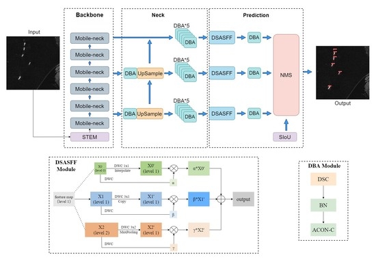
The overview of the proposed LMSD-YOLO is shown in Figure 1 and includes three parts: backbone, neck and prediction. Firstly, the backbone network is composed of Mobile-neck modules and the stem block is placed in front of the backbone. Then, in the neck part, since the path aggregation feature pyramid network (PAFPN) structure can convey the semantic and location information of targets, the extraction ability of multi-scale targets is strengthened. Finally, in order to enhance the multi-scale feature fusion, the DSASFF module is added before the prediction head.

2.1. DBA Module

Traditional convolution blocks usually adopt convolution (Conv) batch normalization (BN) operation and the Leaky Relu (CBL) module for feature extraction, as shown in Figure 2a. In order to obtain a more lightweight network model, we propose a lightweight DBA module as a basic computing unit. The DBA module consists of depthwise separable convolution(DSC)module, BN operation and activate or not (ACON) activation function [25], where the main source of computation is the convolution of the image features, while the BN and activation function have very few parameters. The structure of DBA module is shown in Figure 2b.

We replace the CBL module with the DBA module as a lightweight basic unit in the backbone and neck of the model. Compared with the traditional CBL module, the DBA module proposed in this paper is more lightweight. The DSC module is used to reduce the overall computational load of the module, and the ACON family functions can effectively prevent neuron death in the process of large gradient propagation. The structure of the DSC module is shown in Figure 3.

Compared with the traditional standard convolution operation, the DSC module decomposes the entire convolution operation into two parts: depthwise convolution (DWC) [26] and pointwise convolution (PWC) [27]. The calculation equation of DSC module is denoted as:

$$Output=DSC(input)=PW{C}_{1\times 1}\left\{Conca{t}_{i=1}^{\mathrm{N}}\left[DW{C}_{3\times 3}\left(x_i\right)\right]\right\}$$

(1)

where $x_i$ represents the input features of each channel, $Conca{t}_{i=1}^{\mathrm{N}}$ represents the combination of the feature maps in the channel dimension. Moreover, 3 × 3 and 1 × 1 represent the size of the convolution kernel size used in calculating DWC and PWC, respectively.

In the DWC process, one convolution kernel is responsible for one channel, and one channel is only convolved by one convolution kernel. The number of feature map channels generated by this process is exactly the same as the number of input channels. The operation of PWC is very similar to the traditional convolution operation, using a 1 × 1 × C convolution kernel. Therefore, the PWC operation will perform a weighted summation of the feature map in the depth direction, and compress the feature map in the channel dimension to generate new feature maps.

The Relu [28] activation function is widely used by most neural networks because of its excellent non-saturation and sparsity. However, since the Relu activation function only has a single form, it is difficult to converge the lightweight model during the training stage. In this paper, we adopt a new activation function, ACON activation function, to enhance the fitting and convergence of the model. The classification of ACON family activation functions is shown in Table 1.

Table 1. Summary of the ACON family.

${\mathit{\eta }}_{\mathit{a}}(\mathit{x})$${\mathit{\eta }}_{\mathit{b}}(\mathit{x})$	ACON Family	Function Expression
$x$, 0	ACON-A	$f_{\mathrm{ACON}-\mathrm{A}}(x)=x\cdot \sigma (\beta x)$
$x$$, px$	ACON-B	$f_{\mathrm{ACON}-\mathrm{B}}(x)=(1-p)x\cdot \sigma [\beta (1-p)x]+px$
$p_{1}x$$, p_{2}x$	ACON-C	$f_{\mathrm{ACON}-\mathrm{C}}(x)=\left(p_1-p_2\right)x\cdot \sigma \left[\beta \left(p_1-p_2\right)x\right]+p_{2}x$

Table 1. Summary of the ACON family.

${\mathit{\eta }}_{\mathit{a}}(\mathit{x})$${\mathit{\eta }}_{\mathit{b}}(\mathit{x})$	ACON Family	Function Expression
$x$, 0	ACON-A	$f_{\mathrm{ACON}-\mathrm{A}}(x)=x\cdot \sigma (\beta x)$
$x$$, px$	ACON-B	$f_{\mathrm{ACON}-\mathrm{B}}(x)=(1-p)x\cdot \sigma [\beta (1-p)x]+px$
$p_{1}x$$, p_{2}x$	ACON-C	$f_{\mathrm{ACON}-\mathrm{C}}(x)=\left(p_1-p_2\right)x\cdot \sigma \left[\beta \left(p_1-p_2\right)x\right]+p_{2}x$

• where ${\eta }_a(x)$, ${\eta }_b(x)$ represent the linear function factor. $p$, $p_1$ and $p_2$ represent the change coefficient of the linear function, $\sigma$ denotes the sigmoid activation function and $\beta$ denotes the connection coefficient of the two linear function factors.

In order to accurately describe the linear and nonlinear control of neurons in the ACON activation function, the linear parameters $p_1$ and $p_2$, and the connection coefficient $\beta$ are added as learnable parameters to adaptively learn and update the activation function. ACON-C avoids preventing neuronal necrosis by controlling the upper and lower bounds of the activation function. The first derivative of $f_{\mathrm{ACON}-\mathrm{C}}(x)$ is:

$$\frac{d}{dx}\left[f_{\mathrm{ACON}-\mathrm{C}}(x)\right]=\frac{\left(p_1-p_2\right)\left(1+e^{-\beta \left(p_{1}x-p_{2}x\right)}\right)+\beta {\left(p_1-p_2\right)}^2{e}^{\left.-\beta \left(p_{1}x-p_{2}x\right)\right)}x}{{\left(1+e^{-\beta \left(p_{1}x-p_{2}x\right)}\right)}^2}+p_2$$

(2)

$$\begin{array}{l}\underset{x\to \infty }{lim}\frac{d{f}_{\mathrm{ACON}-\mathrm{C}}(x)}{dx}=p_1\\ \underset{x\to -\infty }{lim}\frac{d{f}_{\mathrm{ACON}-\mathrm{C}}(x)}{dx}=p_2\end{array}$$

(3)

Equation (3) calculates the magnitude of the upper and lower bounds of the first-order derivative of ACON-C. When $x$ tends to positive infinity, the gradient is $p_1$. While x tends to negative infinity, the gradient is $p_2$.

Then, calculating the second derivative of $f_{\mathrm{ACON}-\mathrm{C}}(x)$ is shown as follows:

$$\frac{d^2}{d{x}^2}\left[f_{\mathrm{ACON}-\mathrm{C}}(x)\right]=\frac{\beta {\left(p_2-p_1\right)}^2{\mathrm{e}}^{\beta \left(p_1-p_2\right)x}\left(\left(\beta \left(p_2-p_1\right)x+2\right){\mathrm{e}}^{\beta \left(p_1-p_2\right)x}+\beta \left(p_1-p_2\right)x+2\right)}{{\left({\mathrm{e}}^{\beta \left(p_1-p_2\right)x}+1\right)}^3}$$

(4)

By making Equation (4) equal to 0, the upper and lower bounds of the first derivative are calculated as follows:

$$\begin{array}{l}max\left(\frac{d}{dx}\left[f_{\mathrm{ACON}-\mathrm{C}}(x)\right]\right)\approx 1.0998p_1-0.0998p_2\\ min\left(\frac{d}{dx}\left[f_{\mathrm{ACON}-\mathrm{C}}(x)\right]\right)\approx 1.0998p_2-0.0998p_1\end{array}$$

(5)

As can be seen by Equation (5), the upper and lower bounds for ACON are both related to $p_1$ and $p_2$. Since $p_1$ and $p_2$ are the learnable parameters, a better performing activation function can be obtained during network learning. In this paper, ACON-C is adopted as the activation function, and the implementation process is shown in

Table 2. ACON-C activation function implementation process.

ACON-C Activation Function Implementation Process

Create learnable parameter vectors and randomly initialize $p_1, p_2$; Calculate the mean value of the input features in the channel dimension and the width dimension at the same time; Send the output from the Step 2 through two convolution layers, all pixels in each channel share their weights; Use the sigmoid activation function to activate the output from the Step 3 to obtain $\beta$; Calculate the ACON-C activate function according to Table 1.

:

2.2. Improved Mobilenetv3 Network

In LMSD-YOLO, the backbone of CSPDarknet53 [29] in standard YOLOv5s is replaced by S-Mobilenet. Compared with the CSPdarknet53, the S-Mobilenet has fewer parameters (only 6.2% parameters of the CSPdarknet53) and better feature extraction performance. The structure and parameter settings of S-Mobilenet are shown in

Table 3. The detailed structure of S-Mobilenet, where SE means the squeeze-and-excitation module, NL stands for the type of activation function.

Input	Mod	Stride	Kernel	Hidden	Output	SE	NL
640 × 640 × 3	Stem block	2	3	-	16	×	ACON-C
320 × 320 × 16	Mobile-neck	2	3	16	32	√	Relu
160 × 160 × 32	Mobile-neck	2	3	72	128	×	Relu
80 × 80 × 128	Mobile-neck	2	5	96	64	√	ACON-C
40 × 40 × 64	Mobile-neck	1	5	240	128	√	ACON-C
40 × 40 × 128	Mobile-neck	2	3	120	256	√	ACON-C
40 × 40 × 256	Mobile-neck	2	3	288	512	√	ACON-C

.

The detailed structure of the stem block consists of maxpooling and convolution operations, shown as Figure 4. Convolution operation can only obtain the local feature information of the target, which reduces the description of the input global features. Therefore, a new branch of maxpooling (the kernel size and the stride are both set to 2) is added to enhance the extraction of global feature information without producing new parameters. In order to completely retain the global and local information, the feature maps of the two branches are concatenated in the channel dimension, meanwhile 1 × 1 Conv is adopted to fuse the spatial information and adjust the output channels.

The MobileNet network is a popular lightweight network proposed by Google in 2017 [30], which has been widely used in the field of computer vision as a mainstream lightweight network, and has achieved excellent results. Mobilenetv3 [31] was proposed by A. G. Howard et al. in 2019. The Mobilenetv3 network consists of a stacked set of block modules, and the structure of the Mobile-neck block is shown in Figure 5.

In Figure 5, the DSC module is adopted to reduce the computational complexity of the model, so that the number of groups in the network is equal to the number of channels. Mobilenetv3 adopts an inverted residual structure after the depthwise filter structure. Since the SE structure introduces a certain number of parameters and increases the detection time, Howard et al. [31] reduced the channel of the expansion layer to 1/4 of its original size. In this way, the authors of Mobilenetv3 found the accuracy is improved without increasing the time consumption. In the last layer of the block, 1 × 1 Conv is used to fuse the feature layers of different channels to enhance the utilization of feature information in the spatial dimension. At the same time, ACON-C is used instead of the h-swish function, which further reduces the computational cost.

2.3. DSASFF Module

Generally, the detection performance of the target is improved by constructing complex fusion mechanisms and strategies, such as the dense structure, but the complex structure also brings more parameters, resulting in low detection efficiency [32]. In addition, feature layers of different scales have different contribution weights during fusion. At present, most multi-scale feature fusion strategies are 1:1 fusion according to the output, thus ignoring the difference of target features at different scales, and increasing unnecessary computational overhead.

In order to improve the detection ability of multi-scale targets, the DSASFF module is introduced to enhance the feature expression ability of multi-scale targets. The structure of the DSASFF module is shown in the Figure 6.

The DSASFF module is embedded between the neck and prediction part, and the three scale feature outputs of the neck part are used as the input of the module. The input feature map is set to level $l$$(l\in 0,1,2)$ according to the scale, and its corresponding feature layer is named $x^l$. In this paper, according to the size of input images and the SAR ship targets, level 0, level 1 and level 2 are set to 128, 256 and 512, respectively. For the up-sampling operation on $x^0$, first we use the DSC operation with a kernel size 1 × 1 to compress the number of feature map channels to the same as $x^1$, and then double the size of the feature map by interpolation. A downsampling operation is performed on the feature layer of $x^2$, using a two-dimensional maximum pooling (MaxPool2d) operation, and then the number of channels is unified by adopting a DSC operation with the kernel size 3 × 3 and the stride 2. The output of DSASFF module is denoted as:

$$out={\alpha }^l\cdot x^{0\to l}+{\beta }^l\cdot x^{1\to l}+{\gamma }^l\cdot x^{2\to l}$$

(6)

where $out$ represents the output feature map of the $l$ level, $\alpha$, $\beta$, $\gamma$ correspond to the learnable weight parameters in the feature maps of the $l-1$, $l$ and $l+1$ layers, respectively, which are obtained by applying DSC module as follows.

$$[\alpha ,\beta ,\gamma ]=D\mathrm{S}C[x^0,x^1,x^2]$$

(7)

The range of these parameters is compressed between [0, 1] by SoftMax, and the relationship between the three parameters is satisfied by Equations (8) and (9):

$${\alpha }^l+{\beta }^l+{\gamma }^l=1$$

(8)

$${\alpha }^l=\frac{e^{{\lambda }_{\alpha }^l}}{e^{{\lambda }_{\alpha }^l}+e^{{\lambda }_{\beta }^l}+e^{{\lambda }_{\gamma }^l}}$$

(9)

The definitions of three parameters ${\lambda }_{\alpha }$, ${\lambda }_{\beta }$ and ${\lambda }_{\gamma }$ in Equation (9) can be obtained by computing the parameters in SoftMax when updating the network by back propagation method. The strategy of the DSC module makes the convolution process more efficient. Meanwhile, the DSASFF module not only has multi-scale feature extraction capability, but also reduces a lot of repeated redundant computation.

2.4. Loss Function

SCYLLA-IoU (SIoU) [33] is used as the loss function for bounding box regression. Compared with CIoU, DIoU and GIoU, SIoU considers the matching angle direction and it makes the box regress to the nearest axis (x or y) faster. SIoU loss is defined as:

$$L=W_{box}{L}_{box}+W_{cls}{L}_{cls}$$

(10)

where $L_{box}$ is box regression loss, $L_{cls}$ is focal loss, and $W_{box}$, $W_{cls}$ represent box and classification loss weights respectively.

The $L_{box}$ is further defined as:

$$L_{box}=1-IoU+\frac{L_{\mathrm{dis}}+L_{\mathrm{shape}}}{2}$$

(11)

where $IoU$ represents intersection over union loss, $L_{\mathrm{dis}}$ and $L_{\mathrm{shape}}$ denote distance loss and shape loss, respectively. The $IoU$ loss represents the intersection ratio of the predicted box and the ground truth, which is defined by:

$$IoU=\frac{\left|B\cap B^{GT}\right|}{\left|B\cup B^{GT}\right|}$$

(12)

The mechanism of angle regression is introduced in SIoU and the schematic diagram of border regression is shown in Figure 7.

Where $B$ and $B^{GT}$ are the predicted bounding box and ground-truth box. $\alpha$, $\beta$ are the angles with the horizontal and vertical directions, respectively. $\sigma$ represents the distance between the center of $B$ and $B^{GT}$. $C_w$ and $C_h$ denotes the length and width.

The direction of the regression of the prediction box is determined by the size of the angles. In order to achieve this purpose, we adopt the following strategy for optimizing the angle parameter $\theta$,

$$\theta =\left\{\begin{array}{l}\alpha ,\hspace{1em}\hspace{1em}\hspace{1em}\alpha \le \pi /4\\ \pi /2-\beta , \hspace{1em}\hspace{1em}\mathrm{else}\end{array}\right.$$

(13)

The angle loss ($L_{\mathrm{angle}}$) is calculated by Equations (14)–(17):

$$L_{\mathrm{angle}}=1-2\ast {\sin }^2\left(\arcsin (x)-\pi /4\right)$$

(14)

$$x=\frac{c_h}{\sigma }=\sin (\theta )$$

(15)

$$\sigma =\sqrt{{\left(b_{c_x}^{gt}-b_{c_x}\right)}^2+{\left(b_{c_y}^{gt}-b_{c_y}\right)}^2}$$

(16)

$$c_h=\max \left(b_{c_y}^{gt},b_{c_y}\right)-\min \left(b_{c_y}^{gt},b_{c_y}\right)$$

(17)

Combined with the $L_{\mathrm{angle}}$ above, the distance loss $L_{\mathrm{dis}}$ is redefined and calculated by Equations (18)–(21):

$$L_{\mathrm{dis}}={\displaystyle \sum _{t=x,y}\left(1-e^{-\gamma {\rho }_t}\right)}$$

(18)

$${\rho }_x={\left(\frac{b_{c_x}^{gt}-b_{c_x}}{c_w}\right)}^2$$

(19)

$${\rho }_y={\left(\frac{b_{c_y}^{gt}-b_{c_y}}{c_h}\right)}^2$$

(20)

$$\gamma =2-L_{\mathrm{angle}}$$

(21)

where ${\rho }_x$, ${\rho }_y$ represent the normalized distance errors in the x or y directions respectively. $L_{\mathrm{dis}}$ is also positively related to the size of $\theta$. Considering that the shape of the prediction box also affects the accuracy of the matching, $L_{\mathrm{shape}}$ is calculated as:

$$L_{\mathrm{shape}}={\displaystyle \sum _{t=w,h}{\left(1-e^{-{\omega }_t}\right)}^{\theta }}$$

(22)

$${\omega }_w=\frac{\left|w-w^{gt}\right|}{\max \left(w,w^{gt}\right)}$$

(23)

$${\omega }_h=\frac{\left|h-h^{gt}\right|}{\max \left(h,h^{gt}\right)}$$

(24)

where ${\omega }_w$, ${\omega }_h$ represent the normalization coefficients in the horizontal and vertical directions, respectively, and their definition is expressed as Equations (23) and (24). θ is used to control how much attention is paid in the shape cost. In this paper, θ is set as 4 on three datasets by referring to Gevorgyan’s suggestion [33] and our own experimental analysis results.

2.5. Network Complexity Analysis

Time complexity and space complexity can be used to evaluate and analyze the network model. Time complexity represents the time cost to run the model and is usually measured in floating point operations ($FLOPs$).

The time complexity of the convolutional neural network ($FLOP{\mathrm{s}}_{\mathrm{net} }$) can be obtained by:

$$FLOP{\mathrm{s}}_{\mathrm{net} }={\displaystyle \sum _{l=1}^N{M}_l^2}\cdot K_l^2\cdot C_{l-1}\cdot C_l$$

(25)

where $M_l$ represents the size of the output feature map of the $l–\mathrm{th}$ layer, and $K_l^{}$ represents the area of the convolution kernel. $N$ is the depth of the network, and $l$ is the number of current convolutional layers. $C_l$ represents the number of output channels of the $l–\mathrm{th}$ layer.

The time complexity determines the training and testing time of the model and is the main factor for the real-time performance. Space complexity refers to the total amount of forward propagation and memory exchange completed by the network model, which can be measured by the total number of model parameters ($\mathit{Model}\_\mathit{Params}$). The space complexity of the network model can be divided into two parts: the weight parameters ($\mathit{Weight}\_\mathit{Params}$) and the output feature parameters ($\mathit{Feature}\_\mathit{Params}$) by each layer, i.e.,

$$\mathit{Model}\_\mathit{Params}=\mathit{Weight}\_\mathit{Params}+\mathit{Feature}\_\mathit{Params}$$

(26)

The $Weight\_Params$ represents the sum of the weight parameters corresponding to each layer in the model. The $Feature\_Params$ refers to the computational parameters caused by the input feature map. The calculation process of $Weight\_Params$ and $Feature\_Params$ are shown in Equations (27) and (28).

$$Feature\_Params={\displaystyle \sum _{l=1}^N{M}^2}\cdot C_l$$

(27)

$$Weight\_Params={\displaystyle \sum _{l=1}^N{K}_l^2}\cdot C_{l-1}\cdot C_l$$

(28)

Convolution is an essential operation for the network to complete feature extraction, and the calculation amount ($FLOP{s}_{\mathrm{CONV} }$) of the standard convolution module can be expressed as:

$$FLOP{s}_{\mathrm{CONV} }=C_{in}\cdot C_{out}\cdot K^2\cdot M^2$$

(29)

where $C_{in}$ is the number of input channels and $C_{out}$ is the number of convolution output by the module. DSC can reduce parameters compared with standard convolution operation, especially in the backbone network that uses a large number of standard convolution, the effect of reducing parameters is more obvious. The calculation amount of the DSC ($FLOP{s}_{\mathrm{DSC} }$) operation can be calculated by Equation (30):

$$FLOP{s}_{\mathrm{DSC} }={\mathrm{C}}_{in}\cdot K^2\cdot M^2+{\mathrm{C}}_{in}\cdot {\mathrm{C}}_{out}\cdot K^2$$

(30)

The ratio of the computational effort of DSC operation and standard convolution is calculated by Equation (31):

$$\frac{FLOP{s}_{\mathrm{DSC} }}{FLOP{s}_{\mathrm{CONV}}}=\frac{{\mathrm{C}}_{in}\cdot K^2\cdot M^2+{\mathrm{C}}_{in}\cdot {\mathrm{C}}_{out}\cdot K^2}{C_{in}\cdot C_{out}\cdot K^2\cdot M^2}=\frac{1}{C_{in}}+\frac{1}{K^2}$$

(31)

When we process the input image, the number of input channels ($C_{in}$) is generally relatively much larger than kernel size ($K$), so the ratio of the $FLOP{s}_{\mathrm{DSC} }$ and $FLOP{s}_{\mathrm{CONV}}$ is further reduced. In addition, we perform a computational analysis of the proposed DSASFF module. Two convolution operations are used for the input features to complete the feature extraction and the corresponding weight value calculation respectively. Then the input feature map is multiplied with the weight values to obtain the output features. Therefore, the calculation amount of DSASFF module (only considering the complex calculation effect brought by the convolution operation) can be expressed as

$$FLOP{s}_{\mathrm{DWASFF}}=FLOP{s}_{\mathrm{feature}}\cdot FLOP{s}_{\mathrm{weight}}={\left({\mathrm{C}}_{in}\cdot K^2\cdot M_l{}^2+{\mathrm{C}}_{in}\cdot {\mathrm{C}}_{out}\cdot K^2\right)}^2$$

(32)

where $FLOP{s}_{\mathrm{feature}}$ and $FLOP{s}_{\mathrm{weight}}$ represent the calculation amount of feature extraction and the calculation amount of weight value, respectively, and both of are calculated by the DSC module.

Compared with the standard ASFF module [34], the DSASFF module proposed in this paper can reduce the calculation amount of each layer when the convolution kernel size remains unchanged, which greatly reduces the overall calculation complexity of the model.

3. Experiments

In order to truly reflect on the scenarios of model deployment and operation, we set up a training platform and a testing platform to complete the training and testing tasks for multiple sets of datasets. In the training platform, we used a high-performance graphics host with 1080ti GPU to complete training on different datasets. Then we used the NVIDIA Jetson AGX Xavier mobile development board as the platform to deploy the model and make an accurate evaluation [35].

3.1. Experimental Platform

3.1.1. Training Platform

The experimental training platform is based on the high performance host with Intel Core I7-8700K CPU, 32GB RAM for DDR4 3200MHz, NVIDIA GTX1080ti (11GB) GPU and the operating system is Ubuntu 20.04 LTS. PyTorch 1.8.0 based on Python 3.7 was used as the development language; moreover, CUDA 10.2 and cuDNN 7.6.5 were adopted to accelerate training on the GPU device. The trained model was transplanted to the NVIDIA Jetson AGX Xavier development board for the detection speed test.

3.1.2. Testing Platform

For the testing part of the experiment, we used NVIDIA Jetson AGX Xavier as the development board to achieve ship detection on the mobile device. NVIDIA Jetson AGX Xavier has 512 CUDA processors based on Volta architecture for accelerated visual image processing calculations, 8-core CPU and 32G LPDDR4x memory. Meanwhile, NVIDIA Jetson AGX Xavier features the characteristics of high performance, low power consumption, large memory bandwidth, etc., which is very suitable for mobile equipment to complete the analysis and processing of a large volume of data. We adopted the NVIDIA JetPack SDK based on the ARM architecture as the development environment to install necessary dependencies such as PyTorch, OpenCV and CUDA10.1.

3.2. Datasets

In order to verify the reliability and robustness of the proposed model in this paper, test and verification experiments were carried out on three datasets (SSDD, HRSID and GFSSD) with different slice resolutions. The detailed parameters of the datasets are shown in

Table 4. Partial details of three datasets.

Datasets	SSDD	HRSID	GFSSD
Image numbers	1160	5604	1238
Ship Numbers	2551	16,965	3302
Image Size	500 × 500	800 × 800	1000 × 1000
Scenes	in_shore, off_shore, multi_scale targets, different levels of noise

.

In our experiments, the label files of the original datasets based on VOC format were converted to the txt label files required by YOLOv5, which is convenient for subsequent training and testing. Inspired by relevant research [12,13,23], the training set and testing set of the three datasets were randomly divided with a ratio 8:2.

3.2.1. SSDD

The SAR ship detection dataset (SSDD) [36] is widely used for testing of the detection model, and it mainly consists of 1160 images and a total of 2456 ship targets, provided by Sentinel-1, TerraSAR-X and RadarSat-2 satellites. The image size in the dataset was 500 × 500, the distance resolution was 1~15m, and multiple polarization modes and many complex sea scenes were included. Figure 8a shows the distribution of ship target length and width information on SSDD.

3.2.2. HRSID

The high-resolution SAR images dataset (HRSID) [37] is a public dataset released by Su Hao from the University of Electronic Science and Technology of China in January 2020, and it is mainly used for ship detection, semantic segmentation and instance segmentation tasks in high-resolution SAR images. The dataset was collected by Sentinel-1 and TerraSAR-X, satellites, with a total of 5604 images and 16,965 targets. The resolution of the images in the HRSID dataset was 800 × 800. The ship target information in HRSID is depicted in Figure 8b.

3.2.3. GFSSD

In this paper, we established a multi-scale SAR ship dataset with a more balanced data distribution-GaoFen3 SAR-ship Detection Dataset (GFSDD). GFSDD was collected from the GaoFen3 satellite. The imaging mode was the Sliding Spotlight (SL), and the distance resolution was between 1.7 m and 3 m. The dataset contains many scenarios such as near shore, far sea, multi-scale targets and high noise. There are a total of 1238 images in GFSDD (containing a total of 3302 ship targets) and the size of each image is 1000 × 1000. Figure 8c shows the distribution statistics of ship target length and width information in GFSDD.

Compared with the other two public datasets, it can be seen from Figure 8 that the GFSDD dataset has a more balanced distribution of ship targets with different scales.

3.3. Experimental Details

Since the structure of LMSD-YOLO is based on YOLOv5s, we adopted the experimental results of YOLOv5s as the baseline. In the training stage, the initial learning rate was set to 0.01, and the optimization method was stochastic gradient descent (SGD). The batch size was set to 16, and the k-means clustering was used to obtain multi-scale anchors which match the different datasets. In the testing stage, the threshold of NMS was set to 0.45, and the confidence threshold was set to 0.25. We also set the input image size as 800 × 800 in HRSID, 512 × 512 in SSDD, and 1024 × 1024 in GFSSD, respectively.

3.4. Evaluation Indices

In this paper, precision ($P$), recall ($R$) and mean average precision ($AP$) were used as the evaluation indicators of our proposed model. The precision represents the percentage of ships detected correctly in all detection results, and the recall represents the percentage of ships detected correctly in the ground truth. The calculation of precision and recall are as follows:

$$P=\frac{TP}{TP+FP}$$

(33)

$$R=\frac{TP}{TP+FN}$$

(34)

where $TP$ (true positive) is the number of ship targets detected correctly, $FP$ (false positive) is the number of ship targets detected incorrectly, and $FN$ (false negative) is the number of ship targets that were missed. The AP is the average of the accuracies obtained for IoU at 0.05 intervals between 0.5 and 0.95 and can be calculated by using both precision and recall:

$$AP={\displaystyle {\mathrm{\int }}_0^{1}P}(R)dR$$

(35)

where $P$ denotes the precision, and $R$ denotes the recall. In order to better evaluate the performance of the model on the development board, we also calculate frames per second (FPS), model parameters and floating-point operations per second ($\mathrm{FLOPs}$). The $\mathrm{FPS}$ is defined as:

$$\mathrm{FPS}=1/T$$

(36)

where $T$ is the detection time for a single image. $\mathrm{FPS}$ represents the number of detected images per second on the test platform (the average frame rate in the validation datasets). Both model parameters and $\mathrm{FLOPs}$ reflect the complexity of the model.

4. Results

4.1. Effect of DBA Module

The DBA module maintains the structure of the traditional convolutional feature extraction unit, and reduces the number of module parameters while ensuring good feature extraction capability.

Table 5. Parameters for DBA module and CBL module in backbone and neck parts.

Module Type	Backbone Params (M)	Neck Params (M)
CBL	4.73	2.85
DBA	3.86	1.93

shows the comparison results of parameter amounts using DBA and CBL under different input conditions.

The training process on three datasets using the DBA module is also analyzed, as shown in Figure 9.

From Figure 9, it is seen that using the DBA module can speed up the lightweight model convergence. The experiments were completed by using YOLOv5s and LMSD-YOLO respectively, and the results show that the use of the DBA module accelerated the convergence of the model to a certain extent. The AP tends to be flat and stable in about 100 epochs on the SSDD and HRSID datasets and about 110 epochs on the GFSDD dataset when the DBA module is involved. By contrast, after using the DBA module, the AP starts to converge in 40 epochs (speed up about 60%) on the SSDD and HRSID datasets, while 80 epochs (speed up 28%) on the GFSDD dataset.

Table 6. The test performance for YOLOv5s and LMSD with and without DBA module on SSDD.

Modules	P	R	AP	Params (M)	FLOPs (G)
YOLOv5s	95.3	94.6	96.3	7.2	16.7
YOLOv5s-DBA	94.9	94.3	96.1	6.5	13.8
LMSD	95.8	92.4	97.2	5.3	7.9
LMSD-DBA	96.5	94.1	98.0	3.5	6.6

shows the results of the test performance with and without DBA module. From Table 6, it can be found that YOLOv5s with DBA module can achieve a lighter model with 6.5 M Params and 13.8 G FLOPs (0.7 M reduce of Params and 2.9 G decrease of FLOPs when compared with YOLOv5s without the DBA module).

4.2. Effect of S-Mobilments Module

Table 7. The performance comparison of different backbone structures. All tests use YOLOv5s as the test framework on the SSDD dataset.

Backbone	P	R	AP	Params (M)	FLOPs (G)
Darknet53	93.2	95.8	94.5	61.9	156.3
CspDarknet53	95.3	94.6	97.4	7.2	16.5
Mobilenetv3	94.8	95.2	96.7	3.7	6.4
S-Mobilenet	95.1	94.3	97.8	2.9	5.5

shows the experimental results under different backbone networks based on YOLOv5s. In this paper, compared with the three mainstream backbone networks of Darknet53, CspDarknet53 and Mobilenetv3, the proposed S-Mobilenet has the fewest model parameters (reducing 95.3% compared to Darknet53 and 58.7% with CspDarknet53), and the computational FLOPs is only 5.5 G. Meanwhile, the S-Mobilenet has approximately improved by 0.4% in precision and makes a 0.9% improvement in AP over Mobilenetv3 with fewer parameters. It also confirms that the ability to extract feature from the target is enhanced.

4.3. Effect of DSASFF Module

Table 8. The performance comparison of different feature fusion structures (all tested in SSDD). Weight volume (M) denotes the size of the model weights after training. FPS is used to describe the detection speed, measured in the NVIDIA Jetson AGX Xavier development board.

Neck Method	P	R	AP	Params (M)	FLOPs (G)	Weight Volume (M)	FPS
FPN	95.0	91.8	95.3	7.2	15.9	12.1	36.3
BiFPN	96.7	93.6	96.5	8.7	18.9	17.6	32.1
PANet	96.3	92.0	96.1	7.8	16.5	14.4	35.6
FPN + ASFF	97.5	92.4	97.4	12.6	25.0	25.4	30.7
FPN + DSASFF	96.9	94.1	97.2	8.0	16.9	14.9	34.8

shows the performance of different feature fusion structures. We mainly selected the mainstream feature fusion modules of FPN, BiFPN, PANet and ASFF for comparison.

The DSASFF module can be seen to have lighter model parameters (with 8.0 M Params and 16.9 G FLOPs), which means that a reduction of 36.5% in Params and 32.4% in FLOPs is achieved when compared with the ASFF on YOLOv5s directly. Through the demonstration of experiments, the DSASFF module can reduce the parameters’ expansion as much as possible (reduced 10% compared with BiFPN and 54% compared with ASFF), while enhancing the detection accuracy, indicating the effectiveness of the lightweight network structure of the designed DSASFF module.

5. Discussion

In order to evaluate the performance of LMSD-YOLO, the six indicators: Params, FLOPs, FPS, P, R, AP, were considered on three datasets: SSDD, HRSID and GFSSD. The input images of three datasets were adjusted to 640 × 640. The Params and FLOPs were obtained on the computer with 1080ti GPU, while FPS can be calculated on the NVIDIA Jetson AGX Xavier development board.

Table 9. Comparison of experimental results with six other state-of-the-art methods on SSDD, HRSID and GFSSD. The best result is marked in bold.

Method	Params (M)	FLOPs (G)	FPS	Weight Volume (M)	SSDD			HRSID			GFSSD
					P	R	AP	P	R	AP	P	R	AP
Faster R-CNN [10]	41.4	134.4	6.9	320.2	78.8	92.3	89.1	67.2	90.5	67.6	87.2	80.5	85.6
FCOS [24]	32.1	126.0	15.8	127.8	84.2	92.6	89.5	62.9	86.1	72.7	87.6	82.3	86.8
CenterNet [25]	16.5	72.5	20.9	88.3	83.3	94.3	89.1	65.3	91.3	68.6	86.5	81.1	84.7
SSD-512 [11]	24.3	87.72	18.1	97.2	92.9	88.0	94.1	80.1	83.0	81.5	88.4	85.7	89.2
YOLOv3 [14]	61.9	156.3	16.4	123.6	91.2	92.4	92.5	83.7	83.5	84.3	89.5	84.4	88.6
YOLOv5s	7.2	16.7	35.6	14.4	95.3	94.6	96.3	94.7	89.4	92.6	89.8	87.3	89.0
LMSD-YOLO	3.5	6.6	68.3	7.6	96.5	94.1	98.0	92.7	86.6	93.9	92.3	87.5	91.7

compared the experience results of LMSD-YOLO with six other state-of-the-art methods.

As shown in Table 9, the proposed LMSD-YOLO method has the least model parameters and weight volume and obtains the fastest detection speed (reached 68.3 FPS) in real-time detection. Compared with the baseline method, the LMSD-YOLO has a great improvement in AP (from 96.3% to 98.0% on SSDD, from 92.6% to 93.9% on HRSID and from 89.0% to 91.7% on GFSSD) while the model parameters are only half of the YOLOv5s. The improvement in detection accuracy is attributed to the stem block and DSASFF module in LMSD-YOLO, which strengthen the extraction of multi-scale ship target features and reduce a large number of false alarm rates.

The effectiveness of the proposed LMSD-YOLO for small and multi-scale ship targets in real scenes is verified on SSDD and HRSID datasets. We conducted comparison experiments with the three methods: Faster-RCNN, SSD and YOLOv5s, and the results are shown in Figure 10 and Figure 11.

Figure 10 shows the detection results in two scenarios selected from the SSDD dataset, where scenario 1 contains inshore ship targets and scenario 2 includes small ship targets. The green anchors represent the ground truth of ship targets, the purple anchors denote the results by Faster-RCNN, the yellow anchors represent the results by SSD, the blue anchors represent the results by YOLOv5s and the red anchors indicate the detection results by LMSD-YOLO.

As shown in scenario 1 (a1) of Figure 10, compared with other models, the LMSD-YOLO can accurately detect inshore and small ship targets which are hidden between ships with a higher confidence. In scenario 2 (a2) of Figure 10, the detection results based on Fast-RCNN (b2) and SSD (c2) cannot accurately detect the multi-scale ship targets and produce false alarm targets at the edge of the land. In the detection results of YOLOv5s (d2), although the targets are accurately detected, the method proposed in this paper (e2) has higher confidence in all targets, with an average improvement of 6% and a maximum improvement of 10%.

Figure 11 shows the detection results in two scenarios selected from the HRSID dataset, where scenario 3 consists of multi-scale offshore ship targets with pure sea background and scenario 4 includes small inshore ship targets in river course.

In scenario 3 (a1) of Figure 11, the results show our proposed model can detect all targets accurately, while all the other three models have missed detections for small targets. In scenario 4, because of complex background and small ship targets, one ship target is missed at the edge of the whole image and one small ship target failed detection in Figure 11(b2,c2,d2). The confidence of the detected targets is low using the other three methods (including Fast-RCNN, Fast-RCNN and YOLOv5s). However, the proposed model in this paper has no missed or failed detection and has higher confidence than other methods.

6. Conclusions

In order to solve problems of multi-scale SAR ship target detection and inefficient operation of deployment on the mobile devices, this paper proposed a lightweight algorithm for the fast and accurate detection of multi-scale ship targets. The proposed algorithm was deployed on the NVIDIA Jetson AGX Xavier development board and the ability of real-time detection was also evaluated. Specifically, the DBA module is used as the basic unit of the model to construct the entire model structure, and strengthen the convergence capabilities of the lightweight model with fewer parameters. Meanwhile, the S-Mobilenet module is proposed as the backbone to compress the amount of model parameters and improve the feature extraction ability. In view of the multi-scale characteristics of ship targets, the DSASFF module was proposed and added before the prediction head to learn the different scale features’ information adaptively with fewer parameters. Experiment results on SSDD, HRSID and GFSSD datasets show that the LMSD-YOLO can achieve the highest accuracy with the smallest model parameters when compared with other state-of-the-art methods. In addition, the LMSD-YOLO can meet the requirements of real-time detection.

Our algorithm is currently tested on small scene slices, and there are still difficulties in implementing target detection directly from large-scale SAR images. In the future, an end-to-end lightweight target detection algorithm will be designed in combination with the SAR image segmentation algorithm to enhance the applicability.

References

1. Cerutti-Maori, D.; Klare, J.; Brenner, A.R.; Ender, J.H.G. Wide-Area Traffic Monitoring With the SAR/GMTI System PAMIR. IEEE Trans. Geosci. Remote Sens. 2008, 46, 3019–3030. [Google Scholar] [CrossRef]
2. El-Darymli, K.; Gill, E.W.; Mcguire, P.; Power, D.; Moloney, C. Automatic Target Recognition in Synthetic Aperture Radar Imagery: A State-of-the-Art Review. IEEE Access 2016, 4, 6014–6058. [Google Scholar] [CrossRef]
3. Wang, X.; Cheng, P.; Liu, X.; Uzochukwu, B. Fast and accurate, convolutional neural network based approach for object detection from UAV. In Proceedings of the 44th Annual Conference of the IEEE Industrial Electronics Society, IECON 2018, Washington, DC, USA, 20–23 October 2018; pp. 3171–3175. [Google Scholar]
4. Leng, X.; Ji, K.; Yang, K.; Zou, H. A Bilateral CFAR Algorithm for Ship Detection in SAR Images. IEEE Geosci. Remote Sens. Lett. 2015, 12, 1536–1540. [Google Scholar] [CrossRef]
5. Gong, B.; Wang, Y.; Cui, L.; Xu, L.; Tao, M.; Wang, H.; Hou, Y. On the Ship Wake Simulation for Multi-Frequncy and Mutli-Polarization SAR Imaging. In Proceedings of the 2018 China International SAR Symposium (CISS), Shanghai, China, 10–12 October 2018; pp. 1–6. [Google Scholar]
6. Girshick, R.; Donahue, J.; Darrell, T.; Malik, J. Rich feature hierarchies for accurate object detection and semantic segmentation. In Proceedings of the 27th IEEE Conference on Computer Vision and Pattern Recognition, CVPR 2014, Columbus, OH, USA, 23–28 June 2014; pp. 580–587. [Google Scholar]
7. Girshick, R. Fast R-CNN. In Proceedings of the 2015 IEEE International Conference on Computer Vision (ICCV), Washington, DC, USA, 7–13 December 2015; pp. 1440–1448. [Google Scholar]
8. Ren, S.; He, K.; Girshick, R.; Sun, J. Faster R-CNN: Towards Real-Time Object Detection with Region Proposal Networks. IEEE Trans. Pattern Anal. Mach. Intell. 2017, 39, 1137–1149. [Google Scholar] [CrossRef] [PubMed]
9. Liu, W.; Anguelov, D.; Erhan, D.; Szegedy, C.; Reed, S.; Fu, C.-Y.; Berg, A.C. SSD: Single shot multibox detector. In Proceedings of the 14th European Conference on Computer Vision, ECCV 2016, Amsterdam, The Netherlands, 8–16 October 2016; pp. 21–37. [Google Scholar]
10. Redmon, J.; Divvala, S.; Girshick, R.; Farhadi, A. You only look once: Unified, real-time object detection. In Proceedings of the 29th IEEE Conference on Computer Vision and Pattern Recognition, CVPR 2016, Las Vegas, NV, USA, 26 June–1 July 2016; pp. 779–788. [Google Scholar]
11. Tian, Z.; Shen, C.; Chen, H.; He, T. FCOS: Fully convolutional one-stage object detection. In Proceedings of the 17th IEEE/CVF International Conference on Computer Vision, ICCV 2019, Seoul, Korea, 27 October–2 November 2019; pp. 9626–9635. [Google Scholar]
12. Li, P.; Che, C. SeMo-YOLO: A Multiscale Object Detection Network in Satellite Remote Sensing Images. In Proceedings of the 2021 International Joint Conference on Neural Networks (IJCNN), Shenzhen, China, 18–22 July 2021; pp. 1–8. [Google Scholar]
13. Yu, J.; Wu, T.; Zhang, X.; Zhang, W. An Efficient Lightweight SAR Ship Target Detection Network with Improved Regression Loss Function and Enhanced Feature Information Expression. Sensors 2022, 22, 3447. [Google Scholar] [CrossRef] [PubMed]
14. Yang, X.; Zhang, X.; Wang, N.; Gao, X. A Robust One-Stage Detector for Multiscale Ship Detection with Complex Background in Massive SAR Images. IEEE Trans. Geosci. Remote Sens. 2022, 60, 5217712. [Google Scholar] [CrossRef]
15. Guo, H.; Yang, X.; Wang, N.; Gao, X. A CenterNet++ model for ship detection in SAR images. Pattern Recognit. 2021, 112, 107787. [Google Scholar] [CrossRef]
16. Sun, Z.; Leng, X.; Lei, Y.; Xiong, B.; Ji, K.; Kuang, G. BiFA-YOLO: A Novel YOLO-Based Method for Arbitrary-Oriented Ship Detection in High-Resolution SAR Images. Remote Sens. 2021, 13, 4209. [Google Scholar] [CrossRef]
17. Xiong, G.; Wang, F.; Yu, W.; Truong, T.-K. Spatial Singularity-Exponent-Domain Multiresolution Imaging-Based SAR Ship Target Detection Method. IEEE Trans. Geosci. Remote Sens. 2022, 60, 5215212. [Google Scholar] [CrossRef]
18. Sun, K.; Liang, Y.; Ma, X.; Huai, Y.; Xing, M. DSDet: A Lightweight Densely Connected Sparsely Activated Detector for Ship Target Detection in High-Resolution SAR Images. Remote Sens. 2021, 13, 2743. [Google Scholar] [CrossRef]
19. Miao, T.; Zeng, H.; Yang, W.; Chu, B.; Zou, F.; Ren, W.; Chen, J. An Improved Lightweight RetinaNet for Ship Detection in SAR Images. IEEE J. Sel. Top. Appl. Earth Obs. Remote Sens. 2022, 15, 4667–4679. [Google Scholar] [CrossRef]
20. Chen, S.; Zhan, R.; Wang, W.; Zhang, J. Learning Slimming SAR Ship Object Detector Through Network Pruning and Knowledge Distillation. IEEE J. Sel. Top. Appl. Earth Obs. Remote Sens. 2021, 14, 1267–1282. [Google Scholar] [CrossRef]
21. Fu, Z.; Cao, W.; Li, S. A Lightweight SAR Image Recognition Algorithm Based on Deep Convolutional Neural Network. In Proceedings of the 2022 2nd International Conference on Consumer Electronics and Computer Engineering (ICCECE), Guangzhou, China, 14–16 January 2022; pp. 937–940. [Google Scholar]
22. Huang, Y.; Wang, Z.; Wang, Z.; Zheng, Y.; Jiao, M. Target feature extraction algorithm for SAR images of complex background based on corner estimation. In Proceedings of the 2021 2nd China International SAR Symposium (CISS), Shanghai, China, 3–5 November 2021; pp. 1–4. [Google Scholar]
23. Wen, G.; Cao, P.; Wang, H.; Chen, H.; Liu, X.; Xu, J.; Zaiane, O. MS-SSD: Multi-scale single shot detector for ship detection in remote sensing images. Appl. Intell. 2022, 1–19. [Google Scholar] [CrossRef]
24. Zheng, X.; Feng, Y.; Shi, H.; Zhang, B.; Chen, L. Lightweight convolutional neural network for false alarm elimination in SAR ship detection. In Proceedings of IET International Radar Conference (IET IRC 2020), Chongqing, China, 4–6 November 2020; pp. 287–291. [Google Scholar]
25. Knauss, A.; Damian, D.; Franch, X.; Rook, A.; Müller, H.A.; Thomo, A. ACon: A learning-based approach to deal with uncertainty in contextual requirements at runtime. Inf. Softw. Technol. 2016, 70, 85–99. [Google Scholar] [CrossRef]
26. Ioannou, Y.; Robertson, D.; Cipolla, R.; Criminisi, A. Deep Roots: Improving CNN Efficiency with Hierarchical Filter Groups. In Proceedings of 2017 IEEE Conference on Computer Vision and Pattern Recognition (CVPR), Honolulu, Hawaii, 21–26 July 2017; pp. 5977–5986. [Google Scholar]
27. Song, W.; Liu, Z.; Tian, Y.; Fong, S. Pointwise CNN for 3D Object Classification on Point Cloud. J. Inf. Process. Syst. 2021, 17, 787–800. [Google Scholar] [CrossRef]
28. Khalid, M.; Baber, J.; Kasi, M.K.; Bakhtyar, M.; Devi, V.; Sheikh, N. Empirical Evaluation of Activation Functions in Deep Convolution Neural Network for Facial Expression Recognition. In In Proceedings of the 43rd International Conference on Telecommunications and Signal Processing (TSP), Milan, Italy, 7–9 July 2020; pp. 204–207. [Google Scholar]
29. Zhu, H.; Xie, Y.; Huang, H.; Jing, C.; Rong, Y.; Wang, C. DB-YOLO: A Duplicate Bilateral YOLO Network for Multi-Scale Ship Detection in SAR Images. Sensors 2021, 21, 8146. [Google Scholar] [CrossRef] [PubMed]
30. Howard, A.G.; Zhu, M.; Chen, B.; Kalenichenko, D.; Wang, W.; Weyand, T.; Andreetto, M.; Adam, H. MobileNets: Efficient convolutional neural networks for mobile vision applications. arXiv 2017. Available online: https://arxiv.org/abs/1704.04861 (accessed on 17 April 2017).
31. Howard, A.; Sandler, M.; Chen, B.; Wang, W.; Chen, L.-C.; Tan, M.; Chu, G.; Vasudevan, V.; Zhu, Y.; Pang, R.; et al. Searching for mobileNetV3. In Proceedings of the 17th IEEE/CVF International Conference on Computer Vision, ICCV 2019, Seoul, Korea, 27 October–2 November 2019; pp. 1314–1324. [Google Scholar]
32. Yu, J.; Zhou, G.; Zhou, S.; Qin, M. A Fast and Lightweight Detection Network for Multi-Scale SAR Ship Detection under Complex Backgrounds. Remote Sens. 2021, 14, 31. [Google Scholar] [CrossRef]
33. Gevorgyan, Z. SIoU Loss: More Powerful Learning for Bounding Box Regression. arXiv 2022. [Google Scholar] [CrossRef]
34. Liu, S.; Huang, D.; Wang, Y. Learning spatial fusion for single-shot object detection. arXiv 2019. Available online: https://arxiv.org/abs/1911.09516 (accessed on 25 November 2019).
35. Xu, X.; Zhang, X.; Zhang, T. Lite-YOLOv5: A Lightweight Deep Learning Detector for On-Board Ship Detection in Large-Scene Sentinel-1 SAR Images. Remote Sens. 2022, 14, 1018. [Google Scholar] [CrossRef]
36. Zhang, T.; Zhang, X.; Li, J.; Xu, X.; Wang, B.; Zhan, X.; Xu, Y.; Ke, X.; Zeng, T.; Su, H.; et al. SAR Ship Detection Dataset (SSDD): Official Release and Comprehensive Data Analysis. Remote Sens. 2021, 13, 3690. [Google Scholar] [CrossRef]
37. Wei, S.; Zeng, X.; Qu, Q.; Wang, M.; Su, H.; Shi, J. HRSID: A High-Resolution SAR Images Dataset for Ship Detection and Instance Segmentation. IEEE Access 2020, 8, 120234–120254. [Google Scholar] [CrossRef]
Figure 1. Overall architecture of the proposed LMSD-YOLO.
Remotesensing 14 04801 g001
Figure 2. The detailed structure of the CBL module and DBA module: (a) structure of CBL module; (b) structure of DBA module.
Remotesensing 14 04801 g002
Figure 3. The structure of DSC module.
Remotesensing 14 04801 g003
Figure 4. The structure of stem block.
Remotesensing 14 04801 g004
Figure 5. The structure of Mobile-neck in Mobilenetv3.
Remotesensing 14 04801 g005
Figure 6. The detailed structure of DSASFF module.
Remotesensing 14 04801 g006
Figure 7. Bounding box regression model.
Remotesensing 14 04801 g007
Figure 8. Ship scale information on three datasets: (a) distribution of ship targets ship on SSDD; (b) distribution of ship targets on HRSID; (c) distribution of ship targets on GFSSD.
Remotesensing 14 04801 g008
Figure 9. The training process of the four methods (YOLOv5s, YOLOv5s-DBA, LMSD and LMSD-DBA) on three datasets: (a) training results on SSDD dataset; (b) training results on HRSID dataset; (c) training results on GFSSD dataset.
Remotesensing 14 04801 g009
Figure 10. Visual detection results on SSDD datasets, (a1) and (a2) denote ground truth of targets, (b1) and (b2) are detection results on Faster-RCNN, (c1) and (c2) are detection results on SSD, (d1) and (d2) are detection results on YOLOv5s, (e1) and (e2) represent detection results on LMSD-YOLO, respectively.
Remotesensing 14 04801 g010
Figure 11. Visual detection results on HRSID datasets. (a1) and (a2) denote ground truth of targets, (b1) and (b2) denote detection results on Faster-RCNN, (c2) and (c2) are detection results on SSD, (d1) and (d2) are detection results on YOLOv5s, (e1) and (e2) represent detection results on LMSD-YOLO.
Remotesensing 14 04801 g011