Abstract
We present a novel method for underground cavity detection using cross-borehole ground-penetrating radar (GPR). Modeling the soil-cavity system as a filter allows us to estimate the group dispersion of the GPR signal induced by propagation through a cavity. We adopt a hypothesis-testing approach based on the observed group dispersion and propose a method which allows us to detect cavities with high probability. The proposed method is validated on both simulated and real measurements. Geologic clutter that causes conventional methods to fail has negligible impact on the efficacy of the proposed method, and the proposed method may be combined with conventional methods to provide a more robust and effective cavity-detection solution.
1. Introduction
In this paper, we present a novel method to detect underground cavities using cross-borehole ground-penetrating radar (GPR). The problem of detecting underground cavities has been considered since before the Common Era, yet it remains relevant to this day [1]. Electromagnetic methods, and ground-penetrating radar in particular, have been shown to perform particularly well on this problem [2,3]. Cross-borehole GPR has been used since at least the 1980s [4,5] and continues to be an effective cavity-detection solution today [6].
Cross-borehole GPR measurements generally fall into one of two classes. In zero-offset profiling (ZOP), the transmitter and receiver are raised or lowered through the boreholes together, such that while measurements are taken over a variety of depths, the transmitter and receiver are always at equal depths. In multiple-offset gathers (MOG), the transmitter and receiver sample every pair of depths—for each depth at which the transmitter transmits, the receiver measures the received signal at every depth. In this paper, we focus on cavity detection using ZOP measurements. Note, however, that features which are successful for detection using ZOP measurements are often adapted to compute tomographic inversions on MOG measurements (for instance, the traveltime used on the ZOP problem in, e.g., [4] is used to compute tomographic inversions in [7]; the authors of [8], among others, consider using for tomography the attenuation considered in, e.g., [4]).
The vast majority of cavity-detection methods appear to be based around traveltime (e.g., [4,7,9,10,11]). An earlier arrival of the signal at the receiver suggests that the signal passed through a cavity, as an electromagnetic (EM) wave propagates more quickly in air than it propagates in soil.
Other cavity-detection methods are based upon the total electric field or its magnitude at the receiver. Examples of such cavity-detection methods can be found in [4,12,13,14]. An EM wave is not attenuated while propagating through a cavity as it is while propagating through soil—as is well known (see, e.g., [15]), the attenuation constant vanishes in media with zero conductivity. However, energy will generally be lost when a portion of the wave is reflected away from the receiver at the soil-cavity interface, and in practice this effect tends to dominate. The fact that these two effects influence the total received energy in opposing directions may render this feature more difficult to use effectively. In many cases it is also difficult to accurately measure the received energy [8].
Full-waveform inversions (FWI) [16,17,18,19,20] and machine learning techniques [21,22] have both been increasingly applied to GPR problems in recent years.
When GPR is applied from the surface, it is sometimes possible to detect cavities using the phase reversal of the reflected wave, as shown in [23,24]. This technique cannot be used effectively in cross-borehole GPR, as the measurements received consist predominantly of the transmitted wave, rather than the reflected wave. When the suspected cavity is shallow, surface GPR may have the advantage of not requiring boreholes. Deeper cavities, however, are generally not detectable by surface GPR; in these cases it may be necessary to use borehole GPR [25].
The use of time-frequency methods is proposed in [26,27]. Similarly, Kim and Kim [28] use simulations to exhibit the dispersion induced in a GPR signal by propagation through a cavity. While different sources use the word “dispersion” to refer to a variety of phenomena, in this paper the word “dispersion” is always taken to mean the dependence of wave velocity on frequency.
Propagation through soil has a low-pass filter effect on the spectrum of EM waves. This low-pass effect was used for general cross-borehole GPR problems in [8] and was applied specifically to the cavity-detection problem in [29]. In this paper, we use a model of the soil-cavity system equivalent to that used in [29] to find the low-pass effect and show that this model also predicts group dispersion. Additionally, the technique used in this paper to find the “background” dispersion is similar to that used in [29] to find the background magnitude spectrum.
One especially intriguing cavity-detection method is proposed in [30]. They attempted to detect an underground cavity using ZOP measurements by searching for depths where the wave exhibits an anomalously low traveltime, but found the traveltime anomaly at the depth of the cavity to be small and difficult to detect. When, however, they applied the short-time Fourier transform (STFT) to the signal received at each depth, they found that the early arrival of the components of the signal centered at 40 MHz at the depth of the cavity was easily discernable. The partial explanation of this phenomenon offered by [30] is that at 40 MHz, the half-wavelength in the background medium is approximately equal to the width of the cavity, though it is still unclear exactly how this leads to the effect observed.
In the following section we model the propagation of an EM wave through the soil-cavity system and show how the cavity induces group dispersion. Significantly, we show that in the soil-cavity system studied by [30], the group delay will have a minimum almost exactly at 40 MHz, possibly providing a more complete explanation for the phenomenon they observed. We also demonstrate the efficacy of dispersion-based cavity detection. In Section 4, we motivate and describe our cavity-detection method, and in Section 5 we validate our method on both simulated and real GPR measurements. In Section 6, we discuss our method and show it to be robust to the effects of borehole drift. Finally, we conclude and offer directions for future research.
The problem of detecting cavities in general is overly broad. In this paper, we limit our treatment to cavities which are significantly extended in the direction perpendicular to the line connecting the two boreholes and which have a width of around a meter or two. These are the types of cavities which have been considered in [4,9,13,27,28,30,31,32], among many others. We do not expect our treatment to be valid for detecting small fractures, where diffraction effects might dominate, or for detecting large caverns. These types of cavity-detection problems require their own treatment, which is beyond the scope of this paper.
2. Modeling the Group Delay
Let us assume that the GPR signal can be modeled as a plane wave, and that diffraction at the edges of the cavity can be neglected. Then at a depth at which a cavity exists, the situation is as shown in Figure 1. The wave travels a distance from the transmitter to the soil-air interface, the portion of the wave transmitted across the interface travels a further distance to the air-soil interface, and the portion of the wave transmitted across the interface travels a further distance before arriving at the receiver. At each interface a portion of the wave is also reflected. Note that the transmitter and receiver boreholes themselves are not modelled, as the diameters of the boreholes are assumed to be much smaller than the smallest non-negligible wavelength of the GPR signal; additionally, at the depth of the measurement the transmitter and receiver boreholes are mostly filled not with air but rather by the antennae themselves. In [29], equations were written for the waves and , allowing them to solve that if , then
where is the wave at the receiver borehole, is the propagation constant, is the wavenumber of the wave in free space, is the distance between the boreholes, and are the coefficients of transmission from soil to air and from air to soil, respectively, is the coefficient of reflection from air to soil, and is the imaginary unit. A perhaps simpler way to arrive at the transfer function is to model the soil-cavity system of Figure 1 as a filter, as in Figure 2. Note that the transfer function of this linear system is defined to be the ratio of the frequency-domain signal measured at the receiver borehole to the frequency-domain signal applied at the transmitter borehole. It can be seen that the transfer function of the “Cavity” filter is given by
where is the transfer function modeling the effect of propagation through the distance of soil and is the transfer function modeling the effect of propagation through the distance of soil. If we substitute in and multiply by the assumed applied signal of , we recover (1), showing that (2) is a slight generalization of (1).
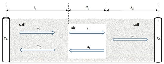
Figure 1.
An EM wave propagates across a cavity between two boreholes. The wave is reflected at every interface.
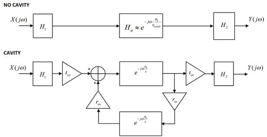
Figure 2.
The propagation of an EM wave across soil that either does or does not contain a cavity, modeled as one of two filters.
Note that (2) does not assume any dispersive properties of the soil, and certainly not of the cavity. Rather, assuming only that the wave is delayed by propagation across the cavity (modeled by the terms) and that the wave is reflected at the air-soil interfaces (modeled by the terms and the feedback), (2) shows that the soil-cavity system will have dispersive properties.
It will be convenient for us to rewrite (2) in terms of , the transfer function modeling propagation of the wave through the soil when no cavity is present. Assuming that the possible cavity has small width, we approximate —that is, we assume that the wave propagates through the distance of soil at the speed regardless of frequency and suffers only negligible attenuation while doing so. This approximation allows us to rewrite (2) as
We now consider the group delay contributed by propagation through the cavity
Approximating the Fresnel coefficients and as real constants independent of frequency, and setting , we can plot for a two-meter-wide cavity, which was the width of the cavity studied in [30]. The resulting plot is shown as Figure 3. Note that the group delay has a minimum almost exactly at 40 MHz. This may better explain the result found in [30], where using the STFT to examine the components of the GPR signal centered at 40 MHz rendered it possible to detect the early arrival of the GPR signal at the depth of the cavity.
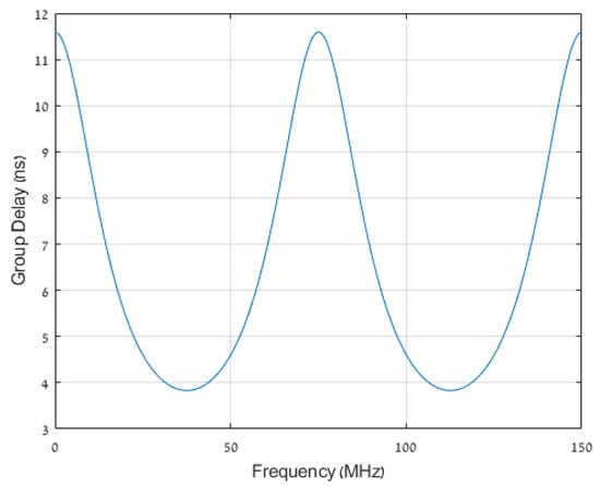
Figure 3.
The group delay contributed by propagation through a two-meter-wide cavity when , as predicted by our model.
In practice, the transmitter and receiver must be close to one another, otherwise the GPR signal will be too attenuated by the time it arrives at the receiver to be detectable. The possible cavity may also be close to the transmitter or receiver. This being the case, it is not clear that it is valid to treat the wave as a plane wave.
To check the validity of (4) in realistic scenarios, we used GPRmax [33,34] to twice simulate GPR measurements in homogeneous soil with a relative permittivity of 10 and conductivity of 0.002 S/m—the parameters given by [35] for both “Dry, sandy coastal land” and “Rocky land, steep hills”. In one of the simulations we added a two-meter-wide cavity, containing only free space, which was both long and tall enough to prevent diffraction of the wave around the cavity. The wave impinged on the cavity at normal incidence. In both cases the transmitter and receiver were separated by 6.8 m and the source wavelet was a derivative of the Gaussian function centered at 30 MHz.
Taking the refractive index n of the soil to be and then applying the Fresnel equations to find the coefficient of reflection between free space and the soil, we find , so our model predicts that the cavity will induce the group delay shown in Figure 3. To find the group delay induced in the measured signal, we measure , where is the Fourier transform of the signal which propagated through the cavity, and is the Fourier transform of the signal which did not pass through a cavity. Measured in this manner, we would expect agreement only up to an additive constant; this is not problematic as we in any event intend to measure only the dispersion induced by the cavity and not its effect on absolute traveltime.
The measured group delay, along with the signals’ magnitude spectra, are shown in Figure 4. The group delay predicted by (4) is far from a perfect fit, but it does seem to be a “qualitative fit”—the predicted and measured group delays have maxima and minima of approximately the same magnitudes and at approximately the same frequencies. Note that at the highest and lowest frequencies, where the fit is quite poor, the simulated signal has little energy; it seems likely that at those frequencies the signal is mostly numerical noise.
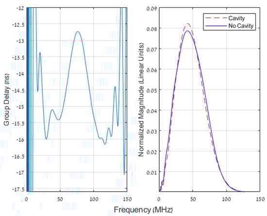
Figure 4.
The group delay contributed by propagation through a two-meter-wide cavity, found using simulated measurements, and the magnitude spectra of the two simulated signals. Note that the results are expected to agree with those shown in Figure 3 only up to an additive constant.
The simulation was then repeated, but the cavity’s height was limited to two meters. The magnitude spectra of the signals and the group delay induced by a cavity are shown in Figure 5. As expected, the fit has degraded from that shown in Figure 4, but it still seems to be a “qualitative fit.” It seems that this fit is more than sufficient for us to use as the basis of hypothesis testing; additionally, we expect that the deleterious effects of diffraction will be “averaged out” if we measure the signal which passes through a cavity at multiple depths relative to the top or bottom of the cavity.
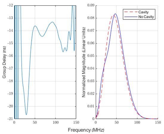
Figure 5.
The group delay contributed by propagation through a cavity, found using simulated measurements, and the magnitude spectra of the two signals. The cavity and soil were identical to those used in Figure 4, other than that the height of the cavity was limited to two meters, thus allowing the wave to diffract around the cavity. Note the slight change in scale from Figure 4.
3. Motivating Dispersion-Based Cavity Detection
Consider the two ZOP profiles shown in Figure 6. The profiles were taken using adjacent pairs of boreholes at a test site characterized by stratified sedimentary rock. Specifically, the test site was located in a geological formation whose strata consist of chert, chalk, limestone, and dolomite. The boreholes used to measure the profile shown on the left do not bracket any cavities, while the boreholes used to measure the profile shown on the right bracket a cavity located at around 19 or 20 m below the surface. This cavity has a width and height of between one and two meters and is significantly extended in the direction orthogonal to the line between the two boreholes. It can be seen that in the right-hand profile, the signal arrives earlier at the depth of the cavity, illustrating how traveltime may be used for cavity detection. Unfortunately, in both profiles the signal also arrives early at around 13 m below the surface, as the stratum at that depth allows the wave to propagate anomalously quickly. Even worse, the signal arrives early at around 19 m below the surface in the left-hand profile as well, showing that another anomalous stratum exists at or adjacent to the depth of the cavity itself. One would be unable to detect the cavity (with a reasonable probability of false alarm) from the right-hand profile alone, and even when using a pair of adjacent profiles it is difficult to detect the cavity without prior knowledge. The difficulty of detecting the cavity using traveltime alone increases with the distance between the transmitter and receiver boreholes; in this case the boreholes are separated by seven meters. When the boreholes were further apart than this we were unable to detect the cavity using traveltime even when comparing profiles taken using adjacent pairs of boreholes (though when the boreholes were only 3.5 m apart we found it quite easy to detect cavities using only traveltime from even only a single profile).
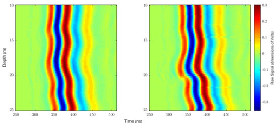
Figure 6.
Two real measured ZOP profiles taken from adjacent pairs of boreholes at the same test site characterized by stratified sedimentary rock. In each profile, the transmitter and receiver boreholes were seven meters apart. The signals measured at each depth were normalized to have unit energy. The boreholes used to measure the profile shown on the left do not bracket any cavities, while the boreholes used to measure the profile shown on the right bracket a cavity located at around 19 or 20 m below the surface. The signals were cropped in order to better show the most relevant portions.
Similarly to [30], we will apply the STFT to the signal measured at each depth in these two profiles. Rather than examining the traveltime of each component of the signal, as did [30], we will examine the difference in traveltime between two components of the signal. Here we will define the traveltime of each component of the signal to be the time at which five percent of its total energy has arrived at the receiver. While [30] examined not the traveltime as we have defined it but rather the time of the first peak, we have found that in our signals the time of the first peak is unacceptably noisy. The results of plotting the differences in traveltime of the components of the signals centered at 40 MHz and the components of the signals centered at 80 MHz for these two profiles are shown in Figure 7.
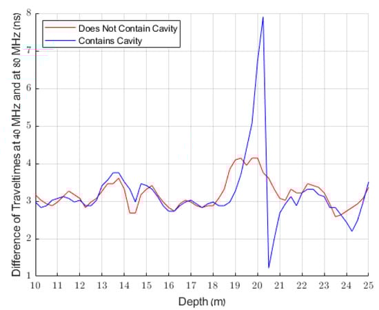
Figure 7.
The difference in traveltime between the component of the signal centered at 40 MHz and the component of the signal centered at 80 MHz, drawn for every depth of the two real measured profiles shown in Figure 6.
If the results shown in Figure 7 are representative (and it appears that they are), then it would appear that cavities can be detected by searching for depths at which the signal experiences anomalous dispersion. Such an approach does indeed seem to be effective. However, since we can use (4) to model the dispersion induced by a cavity, we expect that, as was found by [31], searching for observations which match those predicted by our model will improve the efficacy of our method. This motivates us to adopt a hypothesis-testing approach to cavity detection based on the dispersion of the received signal. This approach is presented in the next section.
4. The Cavity-Detection Method
We assume that in each profile there are exactly zero or one cavities and treat the problem as a hypothesis-testing problem. Let where is the phase, at frequency , of the signal received at depth d, and let be the value that is expected to take on should a cavity not exist. At each depth d, the measured quantity should conform to one of two hypotheses:
where is an arbitrary reference frequency and denotes the noise at frequency at depth d. Note that the factor of on the left-hand side of (3) may be ignored as
is constant for all frequencies.
We now make four additional assumptions:
- The width of the suspected cavity is at least approximately known.
- If a cavity is present, then the wave impinges upon the cavity at approximately normal incidence (or more generally, the angle of incidence is at least approximately known).
- The noise is normally distributed at each and identically distributed for all d.
- The noise at each frequency is independent (the naïve assumption).
The first two assumptions hold in practice. Since the noise is likely mostly due to inhomogeneities in the soil and the failure of the assumptions upon which we built our model, the Central Limit Theorem justifies assuming that the sum of these many disparate sources of error is normally distributed. The normal distribution is also “well-behaved” in the sense that the probability of an observation decreases monotonically with its distance from the mean, so even if the third assumption is less valid we expect that it will not harm our results overmuch.
The final assumption is not at all valid. We would prefer to estimate the full covariance matrix of the noise among the many different frequencies. Since we deal with many frequencies, estimating the covariance or using it to compute probabilities would require inverting large matrices; this is unfortunately computationally intractable. In machine learning and related fields, a similar assumption of the independence of features has been used to deal with similar problems of computational intractability, most notably in the Naïve Bayes algorithms. This assumption is often known as the naïve assumption. Though these algorithms often compute correct classifications, they are often wildly overconfident in their predictions, as they may take each of a large number of correlated features as an independent confirmation of a certain classification. As we make use of a similar naïve assumption, we would expect that the likelihood ratios our method returns will be similarly overconfident; we still hope that our method will return a large value of the likelihood ratio only at the depths at which a cavity exists.
We cannot calculate the likelihood of without knowing (in order to calculate the term), and we cannot calculate the likelihood of either hypothesis without knowing or the variance of . We will deal with the former problem by simply computing the maximum of the likelihood of over , and we will deal with the latter problem by estimating both and the variance of in a manner reminiscent of cell-averaging Constant False Alarm Rate (CA-CFAR) radar.
We slide a small window over all depths in our profile over which we wish to search for a cavity. We measure at each depth in this window, and take the mean value of over all depths d in the window to be the measurement of the depth of the center of the window. This value is comparable to the value measured at the cell under test (CUT) in CFAR radar.
We will ignore all depths which are within a certain guard distance of the window, just as CFAR radar commonly ignore measurements from the guard cells. We designate all depths further than the guard distance from the window as the training depths. For each depth d in the training depths, we measure . The mean value of this quantity over d is taken to be our estimate of . We also compute the sample variance of the measurements in the training depths at each frequency as our estimate of the variance of . We can now compute, for each depth at which the window was centered, the likelihood of and the maximum likelihood of over ; we can then compute the likelihood ratio of the two hypotheses (in practice we compute the difference of the log-likelihoods).
As seen in Section 2, our model unsurprisingly fails when applied to a portion of the spectrum where the signal has little energy. By default, we examine every sampled by the FFT of the received signal only in the portion of the spectrum where all received signals have appreciable energy. As our signals are generally short, closely-spaced will tend to be highly correlated, so we expect that due to the naïve assumption the scale of our results will not be comparable when applied to signals of differing lengths (and the results will similarly certainly not be comparable when applied to signals with different spectra).
A pseudocode description of this method appears in Appendix A.
5. Evaluation and Results
To evaluate the performance of our cavity-detection method, we first used GPRmax to simulate cross-borehole GPR measurements across homogenous soil with a relative permittivity of 10 and conductivity of 0.002 S/m, which are the parameters given by [35] for “Dry, sandy, coastal land”. A cavity (containing only free space) with a width of one meter, significantly extended in length (perpendicular to the line connecting the two boreholes), was placed between the depths of 3.85 and 5.5 m below the surface. The transmitter and receiver were separated by six meters. ZOP measurements were simulated every 0.25 m up to a depth of 10 m. The source waveform was a derivative of the Gaussian function with a center frequency of 30 MHz. The simulated profile is shown in Figure 8, and the results of applying our method to these simulated measurements are shown in Figure 9.
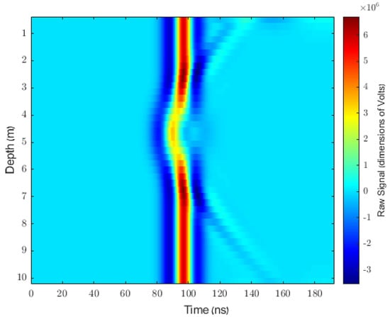
Figure 8.
The profile taken over simulated homogenous soil as described in the text. The signals were cropped to show only the most relevant portions.
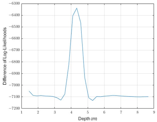
Figure 9.
The results of applying our method to the simulated profile shown in Figure 8. We examined the frequency range of 16–80 MHz, used a window size of four depths (one meter), and used a guard distance of two depths (0.5 m). The cavity was assumed to have a width of one meter.
Though our method clearly succeeded in detecting the simulated cavity, the homogeneous soil was unrealistically simple. Indeed, it can be seen from Figure 8 that the cavity in this case could have been detected just as easily using traveltime-based methods. In an attempt to more accurately model real-world soils, and in particular to model the stratified soils which often challenge traveltime-based methods, we modeled the stratification of soil as a Brownian process and simulated six pairs of profiles, where each profile in the pair is over identical soil other than a cavity which exists in one of the profiles. An example of such a pair of profiles is shown in Figure 10, and the full details of these simulations are given in Appendix B. Note that the faint hyperbolic reflection visible in Figure 8 is not visible in more realistic simulated measurements such as those shown in Figure 10 or in real measurements such as those shown in Figure 6. For this reason, we do not attempt to use this hyperbolic reflection as a feature for cavity detection.
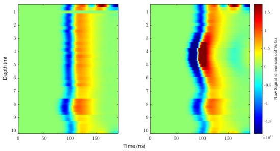
Figure 10.
A representative pair of profiles taken over the simulated stratified soils described in Appendix B. The two profiles were taken over soil which was simulated identically other than the cavity which exists at around four meters below the surface in the profile on the right. The profiles showcased in this figure were used to draw the pair of likelihood-ratio curves shown in the top right-hand corner of Figure 11. The strange behaviour of the signal at the shallowest and deepest depths appears to be the result of numerical artifacts and should have been ignored by our method due to its CFAR-style nature. The signals were cropped to show only the most relevant portions.
The results of applying our method to these simulated profiles are shown in Figure 11. In each case in which a cavity exists, it is located at the depth of the large peak in the likelihood-ratio curve. Furthermore, we see that there are no large values of the likelihood ratio at depths at which a cavity does not exist. It seems that our method is successful at detecting cavities even in this more challenging case.
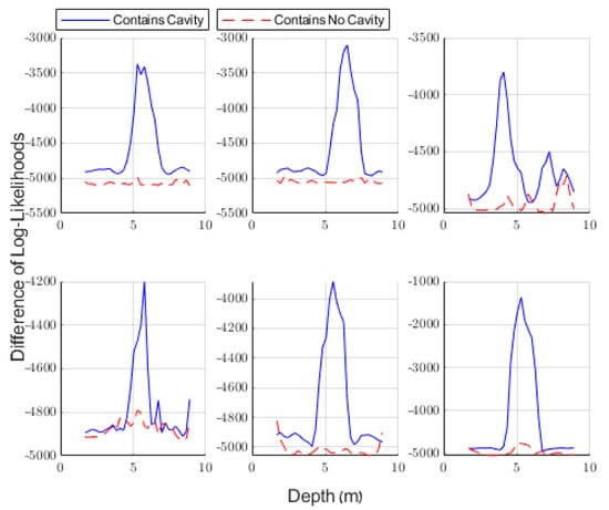
Figure 11.
The results of applying our method to simulated stratified soils. In each case, the cavity is located approximately at the depth of the peak of the solid blue likelihood-ratio curve. We examined the frequency range of 10–55 MHz, used a window size of two depths (0.48 m), and used a guard distance of 8 depths (1.92 m). The cavities were assumed to have a width of 1.5 m.
Finally, we verify the efficacy of our method on several real ZOP measurements taken at a test site characterized by layered sedimentary rock (chert, chalk, limestone, and dolomite). Two profiles typical of the site were shown in Figure 6 and were discussed in Section 3. Eight profiles were taken using pairs of boreholes which did not bracket any cavities, and three profiles were taken using pairs of boreholes which bracketed the same cavity. This single cavity has a cross-section of approximately one square meter and is located at around 19 or 20 m below the surface. Each profile was taken with seven meters between the boreholes. The spectrum of the received signal is centered at around 30–40 MHz depending on the depth. The results of applying our method to these measurements are shown in Figure 12. We see that our method successfully detects the cavity when and only when it exists.
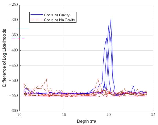
Figure 12.
The results of applying our method to real measurements. The cavity, when it exists, is located around 19 or 20 m below the surface. We examined the frequency range of 36–52 MHz, used a window size of one depth (0.25 m), and used a guard distance of 6 depths (1.5 m). The cavity was assumed to have a width of 1.5 m.
6. Discussion
In this article we deal with the group dispersion, not the traveltime, of the received signal. To this end, we examine the group delay of the received signal at many frequencies relative to the group delay at some reference frequency. It would be trivial to extend our method to work with the absolute group delay. We could, for example, rewrite our two hypotheses as follows:
We could then modify our method to perform hypothesis testing with these refined hypotheses. However, were we to do so we would almost certainly recover results that would be almost indistinguishable from those of conventional traveltime-based methods, as the difference in traveltime would almost always be of greater magnitude than the induced dispersion. What is worse, this method would almost certainly fail when conventional traveltime-based methods fail, such as in cases where there exist strata through which the wave propagates anomalously quickly or slowly—the exact cases on which our method was designed to excel. In particular, we see from Figure 6 and Figure 10 that traveltime-based methods will have difficulty distinguishing the effects of propagating through the true cavity from the effects of propagating through the anomalous strata. This will remain true no matter whether one measures the time of the first peak, as do [4], the time of the maximum of a matched filter, the results of various super-resolution methods, such as those suggested by [36], or the results of any type of manual picking.
Having made the decision to consider only the relative, but not absolute, group delay, it would seem that the results of our method could be combined with the results of conventional traveltime-based methods to yield a more robust cavity-detection solution, as the results of the two methods would be based upon features that are almost entirely independent.
It can be seen from Figure 6 that the received signals in our real measurements exhibit greater traveltime at the deepest depths of the profiles. The centroid frequency of the signals’ spectra also drops by around 2–3 MHz at these depths, and the received energy falls by around 20 dB (though it is possible that, as was found by [8], this measurement of the received energy is noisy). All of these observations are compatible with an increase in the distance between the boreholes. Though we cannot reject the possibility that these effects are simply the results of the properties of the soil at these deepest depths, we conjecture that these effects are at least partially the result of borehole drift.
We would expect group dispersion to be almost unaffected by small perturbations in the distance between the boreholes. A small perturbation in d would affect only the factor of in (1), where , the attenuation constant is real, the phase constant and is the permeability, the permittivity, and the conductivity of the soil. Since
we see that perturbations in d would indeed affect the dispersion, but that for plausible values of , , , and the change in dispersion would be negligible. Figure 13 plots the group delay per meter soil for , = 10, and S/m, which are the same dielectric parameters used in the simulation which generated Figure 8. We see that other than for extremely low frequencies (whose use in GPR is unrealistic), the effect of small perturbations in d on the group dispersion is negligible. Note that for simplicity we have neglected in (5) the frequency-dependence of the dielectric parameters.
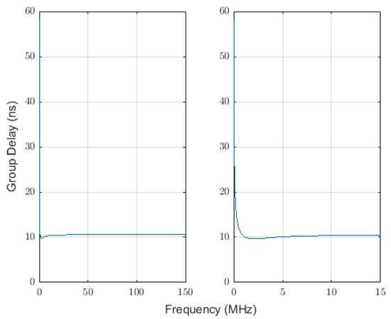
Figure 13.
The group delay per meter soil for , = 10, and S/m. The two plots are the same; the right plot better shows the lowest frequencies.
Indeed, we see from Figure 12 that we do not find anomalous results at the deepest depths of the test site. To further demonstrate that our method is robust to the effects of borehole drift, we twice resimulated the measurements used to generate Figure 8 after adding borehole drift. In both cases the boreholes’ horizontal position deviated from the vertical axis according to a Gaussian function with parameter m and centered at 9.25 m below the surface. In one simulation, the vertical axes of the boreholes were initially separated by six meters, but the boreholes drew closer together such that at 9.25 m below the surface, the boreholes were separated by only approximately 5.2 m. In the other simulation, the boreholes were initially separated by only 5.2 m, but their horizontal positions diverged such that at 9.25 m below the surface, the boreholes were separated by approximately six meters. The measurements from each of the simulations are shown in Figure 14, and the results of our method on these simulations are shown in Figure 15.
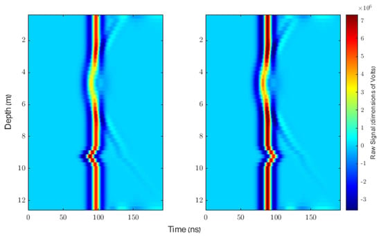
Figure 14.
The profiles of the two simulations described in the text. In each case, the soil was homogenous soil with a relative permittivity of 10 and conductivity of 0.002 S/m. Measurements were simulated every 0.25 m. A cavity having a width of one meter exists between the depths of 3.85 and 5.5 m below the surface, and the borehole drift was most extreme at 9.25 m below the surface. The boreholes simulated in the left-hand profile converge, while the boreholes simulated in the right-hand profile diverge. The signals were cropped to show only the most relevant portions.
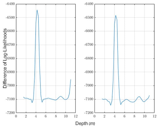
Figure 15.
The results of our applying our method to the simulations shown in Figure 14. In both cases we examined the frequency range of 16–80 MHz, used a window size of four depths (one meter), and used a guard distance of two depths (0.5 m). The cavity was assumed to have a width of one meter.
In the left-hand profile of Figure 14, two traveltime minima can be seen. One is caused by the presence of the cavity, and the other is caused by borehole drift. Without prior knowledge it would be difficult to conclude, based on traveltime alone, that the upper minimum is caused by a cavity and the lower minimum is not. Yet as can be seen from the left-hand plot of Figure 15, our method correctly detects the cavity and is almost unaffected by the borehole drift. Similarly, we see from the right-hand plot of Figure 15 that our method succeeds in detecting the cavity from the right-hand profile in Figure 14 and is almost unaffected by the borehole drift. We conclude that our method, unlike every other method of which we are aware, is robust with respect to borehole drift.
7. Conclusions
We modeled the propagation of a GPR signal through soil which does or does not contain a cavity as one of two filters. It was found that the two filters would induce different group dispersion in the GPR signal. We presented a method to perform hypothesis testing based on the observed group dispersion, and this method was shown to be successful on both simulated and real GPR measurements. Furthermore, this method was shown to be successful even in scenarios where conventional cavity-detection methods fail, such as in the presence of anomalous strata, and it was shown that this method, in contrast to conventional methods, is robust with respect to borehole drift.
The group dispersion considered seems to be relatively independent of other features commonly used for cavity detection, such as traveltime or received energy. It therefore seems likely that the method presented here could be combined with existing methods for a more robust cavity-detection solution. We leave the problem of how best to do this for future research.
We have here considered only the detection of cavities using ZOP measurements. It seems likely that group dispersion would also be an effective feature for localizing the cavity horizontally or for performing tomographic inversions on MOG measurements. As we have seen, the group dispersion is influenced by the relative positions of the walls of the cavity. It is therefore in some sense a nonlocal property, so conventional tomographic inversion algorithms based around integrating some local property of the medium (generally slowness or opacity) over the path of a ray would be difficult to adapt to work with group dispersion. We believe that using the group dispersion for tomographic inversions will prove to be a fruitful direction for future research.
Author Contributions
Conceptualization, C.L. and A.J.W.; Data curation, C.L.; Formal analysis, C.L.; Funding acquisition, A.J.W.; Investigation, C.L.; Methodology, C.L. and A.J.W.; Project administration, A.J.W.; Resources, A.J.W.; Software, C.L.; Supervision, A.J.W.; Validation, C.L.; Visualization, C.L.; Writing—original draft, C.L.; Writing—review and editing, A.J.W. All authors have read and agreed to the published version of the manuscript.
Funding
This research received no external funding.
Data Availability Statement
The input files used to produce the simulations discussed in this paper appear as supplemental material to this paper. The real measurements discussed in this paper are the proprietary data of a third party.
Acknowledgments
We thank Elchanan Zucker for his insightful comments on a previous draft of this work.
Conflicts of Interest
The authors declare no conflict of interest.
Appendix A. A Pseudocode Description of the Cavity-Detection Method
A pseudocode description of the method described in Section 4 is shown as Algorithm A1.

Here we take to be the PDF of the Gaussian distribution with mean and variance , evaluated at x. Note that the maximum is taken over all in line 10 because the Fresnel coefficients used to calculate are functions of the refractive index n of the soil.
Appendix B. The Simulated Stratified Soil
Early on in our research, it became apparent that the results of our cavity-detection methods on simulated soils did not reflect their results on real measurements. While this was unsurprising for naive homogeneous soils such as that used to generate Figure 8, it remained true even for simulated soils based on a fractal mixing model. Much of the difficulty of the cavity-detection problem seems to be influenced by the stratified nature of many real soils. To that end, we elected to explicitly model stratification as a Brownian process.
The parameters for the Brownian process are based off of Table 1 in [37]. The relevant portion of Table 1 consists of the percentages of medium sand, fine sand, very fine sand, coarse-medium silt, and “fine silt + clay.” The measurements were taken at irregularly-spaced depths at various locations. While [37] do not explain why they chose to measure at the depths they recorded, we assume that they recorded the measurements whenever the properties of the soil changed. We therefore take the height of a stratum to be the difference between successive depths measured at a single site. The implementation of the fractal Peplinski model of [38] in GPRmax takes only “sand fraction” and “clay fraction” (with the silt fraction presumably being the remainder of the soil); since GPRmax does not distinguish between the different gradations of sand we take the “sand fraction” to be the sum of the medium, fine, and very fine sand percentages (divided by one hundred). We similarly take the clay fraction to be the “fine silt + clay” percentage (divided by one hundred)—that is, we identify “fine silt + clay” as being entirely clay. Statistics for these parameters are summarized in Table A1. The statistics for the depths of the strata and the change in composition between adjacent strata were determined using 44 measurements, while the mean sand and clay percentages were determined using 58 measurements.

Table A1.
Summary of the statistics used to simulate soils.
Table A1.
Summary of the statistics used to simulate soils.
| Mean Height of Stratum (m) | 1.694 |
| Variance of Height of Stratum (m2) | 1.531 |
| Mean Squared Change in Sand Percentage Between Adjacent Strata | 34.808 |
| Mean Squared Change in Clay Percentage Between Adjacent Strata | 14.7313 |
| Mean Sand Percentage | 89.564 |
| Mean Clay Percentage | 8.274 |
The Peplinski model in GPRmax also takes as parameters the bulk density of the soil, the density of sand particles of the soil, and the range of water volumetric fraction. To estimate these quantities, we used Table 4 in [39]. For a (solid volume) ratio of “fine sand” to “silty clay,” Table 4 in [39] gives the “mean particle density”; we identify “fine sand” with the sand fraction we determined above, “silty clay” with the clay fraction we determined above, and “mean particle density” to be the density of sand particles in GPRmax’s implementation of the Peplinski model. Additionally, Table 4 in [39] gives a minimum and maximum bulk density for a given ratio of fine sand to silty clay and percent “water content” at these bulk densities; we assume that percent “water content” refers to the water volumetric fraction (multiplied by 100).
Finally, we assumed that each stratum is a fractal with a fractal dimension of 1.5, equally weighted in all directions, with 50 different materials (that is, it is made up of 50 fractally-distributed soils, where the difference between the soils is the volumetric water content).
To simulate a profile, we first drew random heights distributed as until the total height met or exceeded the height of the simulation (11 m). These were the heights for each stratum (other than the final height, which may have been clipped). Note that these heights were all drawn from the same distribution.
For each stratum, we drew a random value for the sand and clay percentages from independent normal distributions with variances of 34.808 and 14.7313, respectively. The means for each distribution were the values of the sand and clay percentages from the preceding stratum; in the case of the first stratum the means were 89.564 and 8.274, respectively. The values were clipped to prevent either of them from becoming less than zero or their sum from exceeding 100.
Once the sand and clay fractions had been determined, we found the row in Table 4 in [39] whose sand-to-clay ratio is closest to the ratio drawn for a given stratum. The bulk density for the stratum was drawn from a uniform distribution between the minimum and maximum bulk densities given for that ratio of sand to clay. The range of water volumetric fractions for the stratum was taken to be the water fraction given in Table 4 in [39] for minimum bulk density to the water fraction given for maximum bulk density.
We took measurements every 0.24 m in depth, where the transmitter and receiver were separated horizontally by six meters. The transmitter was a Hertzian dipole, and the voltage across it was a derivative of a Gaussian waveform centered at 30 MHz. After simulating each scenario without a cavity, we simulated measurements in identical soil but with a cavity (containing only free space) added. The cavity’s position was drawn uniformly such that it began at a depth of between 3 to 6 m below the surface and began 1.5 to 3 m from the transmitter. The cavity’s width and height were drawn uniformly and independently to be between one and two meters.
References
- Sloan, S.D.; Miller, R.D.; Steeples, D.W. A history of tunnels and using active seismic methods to find them. Geophysics 2021, 86, WA49–WA57. [Google Scholar] [CrossRef]
- Jabrane, O.; Azzab, D.E.; Himi, M.; Charroud, M.; Gettafi, M.E. Detection of underground cavities using electromagnetic GPR method in Bhalil City (Morocco). In Proceedings of the International Conference on Digital Technologies and Applications, Fes, Morocco, 28–30 January 2021; pp. 1111–1120. [Google Scholar]
- Duff, B. A review of electromagnetic methods used for detection of underground tunnels and cavities. In Proceedings of the 1983 Antennas and Propagation Society International Symposium, Houston, TX, USA, 23–26 May 1983; Volume 21, pp. 634–638. [Google Scholar]
- Kim, S.W.; Kim, S.Y. Analysis of cross-borehole pulse radar signatures measured at various tunnel angles. Explor. Geophys. 2010, 41, 96–101. [Google Scholar] [CrossRef]
- Vesecky, J.; Nierenberg, W.; Despain, A. Tunnel Detection; Technical Report; SRI International: Arlington, VA, USA, 1980. [Google Scholar]
- Diamanti, N.; Annan, A.P. Understanding the use of ground-penetrating radar for assessing clandestine tunnel detection. Lead. Edge 2019, 38, 453–459. [Google Scholar] [CrossRef]
- Berryman, J.G. Stable iterative reconstruction algorithm for nonlinear traveltime tomography. Inverse Probl. 1990, 6, 21. [Google Scholar] [CrossRef]
- Liu, L.; Lane, J.W.; Quan, Y. Radar attenuation tomography using the centroid frequency downshift method. J. Appl. Geophys. 1998, 40, 105–116. [Google Scholar] [CrossRef]
- Alleman, T.; Cameron, C.; MacLean, H. PEMSS response of rock tunnels to “in-axis” and other nonperpendicular antennae orientations. In Proceedings of the 4th Tunnel Detection Symposium on Subsurface Exploration Technology, Golden, CO, USA, 26–29 April 1993; pp. 19–44. [Google Scholar]
- Göktürkler, G.; Balkaya, Ç. Traveltime tomography of crosshole radar data without ray tracing. J. Appl. Geophys. 2010, 72, 213–224. [Google Scholar] [CrossRef]
- Zhou, H.; Sato, M. Subsurface cavity imaging by crosshole borehole radar measurements. IEEE Trans. Geosci. Remote Sens. 2004, 42, 335–341. [Google Scholar] [CrossRef]
- Jia, H.; Takenaka, T.; Tanaka, T. Time-domain inverse scattering method for cross-borehole radar imaging. IEEE Trans. Geosci. Remote Sens. 2002, 40, 1640–1647. [Google Scholar] [CrossRef]
- Ellis, G.A.; Peden, I.C. Cross-borehole sensing: Identification and localization of underground tunnels in the presence of a horizontal stratification. IEEE Trans. Geosci. Remote Sens. 1997, 35, 756–761. [Google Scholar] [CrossRef]
- Côte, P.; Degauque, P.; Lagabrielle, R.; Levent, N. Detection of underground cavities with monofrequency electromagnetic tomography between boreholes in the frequency range 100 MHz to 1 GHz1. Geophys. Prospect. 1995, 43, 1083–1107. [Google Scholar] [CrossRef]
- Thidé, B. Electromagnetic Field Theory; Upsilon Books: Uppsala, Sweden, 2004. [Google Scholar]
- Cordua, K.S.; Hansen, T.M.; Mosegaard, K. Monte Carlo full-waveform inversion of crosshole GPR data using multiple-point geostatistical a priori information. Geophysics 2012, 77, H19–H31. [Google Scholar] [CrossRef]
- Ernst, J.R.; Holliger, K.; Maurer, H. Full-waveform inversion of crosshole georadar data. In SEG Technical Program Expanded Abstracts 2005; Society of Exploration Geophysicists: Tulsa, OK, USA, 2005; pp. 2573–2576. [Google Scholar]
- Ernst, J.R.; Maurer, H.; Green, A.G.; Holliger, K. Full-waveform inversion of crosshole radar data based on 2-D finite-difference time-domain solutions of Maxwell’s equations. IEEE Trans. Geosci. Remote Sens. 2007, 45, 2807–2828. [Google Scholar] [CrossRef]
- Lavoué, F.; Brossier, R.; Métivier, L.; Garambois, S.; Virieux, J. Two-dimensional permittivity and conductivity imaging by full waveform inversion of multioffset GPR data: A frequency-domain quasi-Newton approach. Geophys. J. Int. 2014, 197, 248–268. [Google Scholar] [CrossRef]
- Klotzsche, A.; Van der Kruk, J.; Mozaffari, A.; Gueting, N.; Vereecken, H. Crosshole GPR full-waveform inversion and waveguide amplitude analysis: Recent developments and new challenges. In Proceedings of the 2015 8th International Workshop on Advanced Ground Penetrating Radar (IWAGPR), Florence, Italy, 7–10 July 2015; pp. 1–6. [Google Scholar]
- Liu, B.; Ren, Y.; Liu, H.; Xu, H.; Wang, Z.; Cohn, A.G.; Jiang, P. GPRInvNet: Deep learning-based ground-penetrating radar data inversion for tunnel linings. IEEE Trans. Geosci. Remote Sens. 2021, 59, 8305–8325. [Google Scholar] [CrossRef]
- Travassos, X.L.; Avila, S.L.; Ida, N. Artificial neural networks and machine learning techniques applied to ground penetrating radar: A review. Appl. Comput. Inform. 2020, 17, 296–308. [Google Scholar] [CrossRef]
- Miyamoto, H.; Haruyama, J.; Kobayashi, T.; Suzuki, K.; Okada, T.; Nishibori, T.; Showman, A.P.; Lorenz, R.; Mogi, K.; Crown, D.A.; et al. Mapping the structure and depth of lava tubes using ground penetrating radar. Geophys. Res. Lett. 2005, 32, L21316. [Google Scholar] [CrossRef]
- Ding, C.; Xiao, Z.; Su, Y. A potential subsurface cavity in the continuous ejecta deposits of the Ziwei crater discovered by the Chang’E-3 mission. Earth Planets Space 2021, 73, 53. [Google Scholar] [CrossRef]
- Miwa, T.; Sato, M.; Niitsuma, H. Subsurface fracture measurement with polarimetric borehole radar. IEEE Trans. Geosci. Remote Sens. 1999, 37, 828–837. [Google Scholar] [CrossRef]
- Harkat, H.; Dosse, S.B.; Slimani, A. Time-Frequency Analysis of GPR Signal for Cavities Detection Application. In Proceedings of the Mediterranean Conference on Information & Communication Technologies, Saidia, Morocco, 7–9 May 2015; pp. 107–117. [Google Scholar]
- Duff, B.; Zook, B. Time-frequency representations applied to analysis of hole-to-hole electromagnetic data. In Proceedings of the 4th Tunnel Detection Symposium Subsurface Exploration Technology, Golden, CO, USA, 26–29 April 1993; pp. 221–252. [Google Scholar]
- Kim, S.W.; Kim, S.Y. Analysis of dispersion of pulse signals in underground tunnels using finite-difference time domain and short-time fourier transform. In Proceedings of the XIII Internarional Conference on Ground Penetrating Radar, Lecce, Italy, 21–25 June 2010; pp. 1–5. [Google Scholar]
- Leibowitz, C.; Weiss, A.J. Underground Cavity Detection Through Spectral Distortion of a GPR Signal. IEEE Trans. Geosci. Remote Sens. 2022, 60, 1–8. [Google Scholar] [CrossRef]
- Kim, S.W.; Kim, S.Y.; Nam, S. Short-time Fourier transform of deeply located tunnel signatures measured by cross-borehole pulse radar. IEEE Geosci. Remote Sens. Lett. 2011, 8, 493–496. [Google Scholar] [CrossRef]
- Witten, A. The application of a maximum likelihood estimator to tunnel detection. Inverse Probl. 1991, 7, L49. [Google Scholar] [CrossRef]
- Se-Yun, K.; Ra, J.W. The role of cross borehole radar in the discovery of ’fourth tunnel’ at the Korean DMZ. In Proceedings of the Technical Symposium on Tunnel Detection, Golden, CO, USA, 26–29 April 1993. [Google Scholar]
- Warren, C.; Giannopoulos, A.; Giannakis, I. An advanced GPR modelling framework: The next generation of gprMax. In Proceedings of the 2015 8th International Workshop on Advanced Ground Penetrating Radar (IWAGPR), Florence, Italy, 7–10 July 2015; pp. 1–4. [Google Scholar]
- Giannopoulos, A. Modelling ground penetrating radar by GprMax. Constr. Build. Mater. 2005, 19, 755–762. [Google Scholar] [CrossRef]
- Vance, E.F. Coupling to Shielded Cables; Wiley: Hoboken, NJ, USA, 1978. [Google Scholar]
- Shrestha, S.M.; Arai, I. Signal processing of ground penetrating radar using spectral estimation techniques to estimate the position of buried targets. EURASIP J. Adv. Signal Process. 2003, 2003, 970543. [Google Scholar] [CrossRef]
- Roskin, J.; Katra, I.; Blumberg, D.G. Particle-size fractionation of eolian sand along the Sinai–Negev erg of Egypt and Israel. Bulletin 2014, 126, 47–65. [Google Scholar] [CrossRef]
- Peplinski, N.R.; Ulaby, F.T.; Dobson, M.C. Dielectric properties of soils in the 0.3–1.3-GHz range. IEEE Trans. Geosci. Remote Sens. 1995, 33, 803–807. [Google Scholar] [CrossRef]
- Bodman, G.; Constantin, G. Influence of particle size distribution in soil compaction. Hilgardia 1965, 36, 567–591. [Google Scholar] [CrossRef]


Publisher’s Note: MDPI stays neutral with regard to jurisdictional claims in published maps and institutional affiliations. |
© 2022 by the authors. Licensee MDPI, Basel, Switzerland. This article is an open access article distributed under the terms and conditions of the Creative Commons Attribution (CC BY) license (https://creativecommons.org/licenses/by/4.0/).