Time Series Analysis-Based Long-Term Onboard Radiometric Calibration Coefficient Correction and Validation for the HY-1C Satellite Calibration Spectrometer

Abstract

The HY-1C Satellite Calibration Spectrometer (SCS) is designed for high-accuracy and high-frequency cross-calibration for sensors mounted on the HY-1C satellite; thus, its onboard calibration consistency and stability are crucial for application. Most onboard calibration errors can be corrected via observation physical models and the prelaunch calibration process. However, the practical SCS calibration coefficient still retains some regularity, which indicates the existence of residual calibration errors. Therefore, in this study, a time series analysis-based method is proposed to eliminate this residual error. First, the SCS onboard calibration method and coefficients are described; second, a seasonal–trend decomposition based on the Loess (STL) method is used to model the SCS calibration coefficient; third, the calibration coefficient is validated, corrected and predicted using the constructed STL model; and finally, a long short-term memory (LSTM) neural network method is also used to model and forecast the calibration coefficient. The analysis results show that: 1. the STL method can effectively model, interpret and correct the SCS calibration coefficient error; and 2. the LSTM method can also fit and forecast the calibration coefficients, while its accuracy and interpretability are poor. The proposed methods provide a data analysis-based perspective to monitor remote sensors and help improve the calibration accuracy.

1. Introduction

Ocean satellite remote sensing has the unique advantages of all-day, all-weather, large-scale and long-term observations. Therefore, it is widely used for ocean research, such as primary ocean productivity estimation [1], coastal suspended sediment monitoring [2], red tide monitoring [3], fishery development monitoring [4] and ocean environment monitoring [5]. Ocean color remote sensing uses the water-leaving radiance signals of remote sensors and the water body bio-optical model to invert the water body optical component concentration. Therefore, the calibration accuracy of ocean color sensors is crucial for high-accuracy remote sensing applications [6,7,8].

At present, the in-orbit calibration methods of ocean color remote sensors include cross-calibration, vicarious calibration and onboard calibration. Cross-calibration refers to using the data of mainstream well-calibrated sensors (such as MODIS [9] and VIIRS [10]) as a standard reference to calibrate the undetermined sensors in their cross-observation region. The accuracy of this method is limited by the differences in the spectral response, spatial resolution and observation time between the two sensors. The vicarious calibration method uses the observation data obtained from the Hawaii MOBY buoy [11] to calibrate the sensors, but it is limited by weather conditions, site conditions, measurement accuracy, measurement period and some other factors of on-site observations. Onboard calibration refers to using a specially designed calibration device mounted on the satellite to calibrate the sensors. This method can ensure the reliability of the calibration source and observation conditions. The onboard calibration method has the advantages of high calibration frequency and accuracy. Therefore, most ocean color remote sensors are equipped with onboard calibration devices to monitor and correct their long-term spectral and radiometric response changes to ensure remote sensing data accuracy.

At present, onboard radiometric monitoring and calibration methods are based on an observation physical model of remote sensors and the onboard calibration module [12,13,14]. Such methods are clear in principle and easy to implement but, in practice, the radiometric calibration coefficients of remote sensors often retain some regularity after correction based on the physical observation model [15,16,17]. According to the measurement theory, if the calibration errors caused by the observation condition and the calibration source are well corrected, then the residual calibration coefficient error should only be caused by the onboard calibration module and the instrument itself. In this case, well-corrected onboard calibration coefficients should have the same measurement error distribution as that calibrated in the lab before launch, and if the remote sensors are well calibrated in the lab, their measurement error should be subject to a Gaussian random distribution. Therefore, the nonrandomness of the calibration coefficients is widely believed to be caused by an unknown observation geometry error such as a pointing angle error of the calibration modules and orbit position errors [15,16,17,18,19]. Usually, these observation model-based calibration data can only be corrected using empirical methods such as smoothing or function fitting before they can be used as the best estimation of the onboard calibration coefficients. This type of method is relatively arbitrary, so its generalization ability and correction accuracy are difficult to evaluate.

Therefore, we want to use a pure data-driven time series analysis method to model and analyze the in-orbit calibration coefficients based on statistical knowledge, and in turn to evaluate and eliminate the residual system error of the onboard calibration coefficients, and finally improve the calibration accuracy of the remote sensors.

As a common data form, time series have been widely used for research and applications in fields such as meteorology, finance, hydrology and electricity [20,21,22,23]. The time series analysis method is also widely used for the long-term monitoring of ground features and the consistency and accuracy validation of remote sensors [24,25,26,27]. However, pure data-driven analysis and data processing methods are seldom used for the in-orbit monitoring and calibration of remote sensors. The onboard radiometric calibration coefficients of remote sensors are typical time series data, which implies the characteristics of the sensors, the onboard radiometric calibration module and the relative relationship between them. Therefore, the observation physical model-based onboard calibration coefficients can be analyzed and corrected using the time series analysis method. This method may be able to obtain a significant amount of information about the sensor and its calibration process, and is helpful to monitor and analyze the onboard status of the sensor. In addition, the time series model can be used as additional reference information for the forecast and validation of the onboard radiometric calibration coefficients.

Therefore, in this paper, we use time series analysis-based methods to analyze and correct the long-term onboard radiometric calibration coefficients of the HY-1C Satellite Calibration Spectrometer (SCS) from launch days 8 September 2018 to 7 April 2022. Section 2 introduces the HY-1C satellite and its onboard calibration method and the time series analysis methods used for calibration coefficient analysis and correction in this study. Section 3 describes the time series analysis-based calibration coefficient analysis and correction results and provides a discussion of the constructed time series models. Section 4 summarizes the main results and findings of this study and gives a perspective of the proposed calibration data processing methods.

2. Materials and Methods

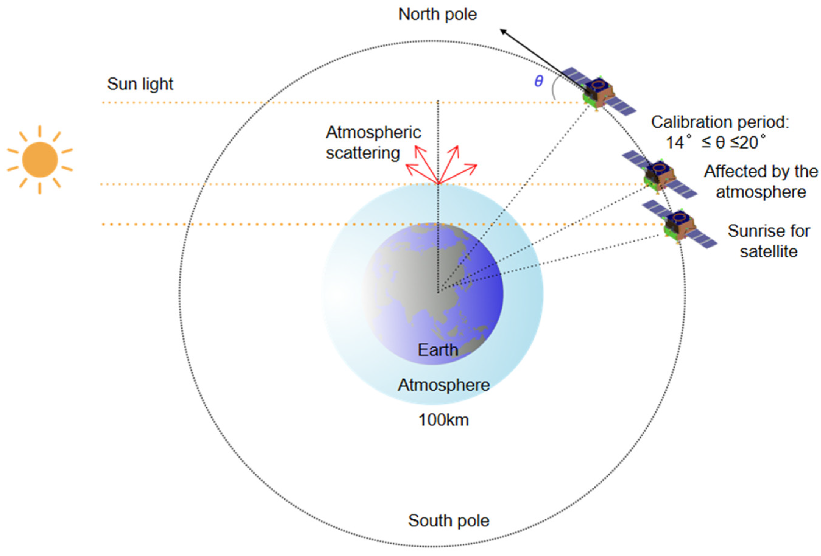
2.1. Overview of Onboard Calibration of HY-1C Sensor

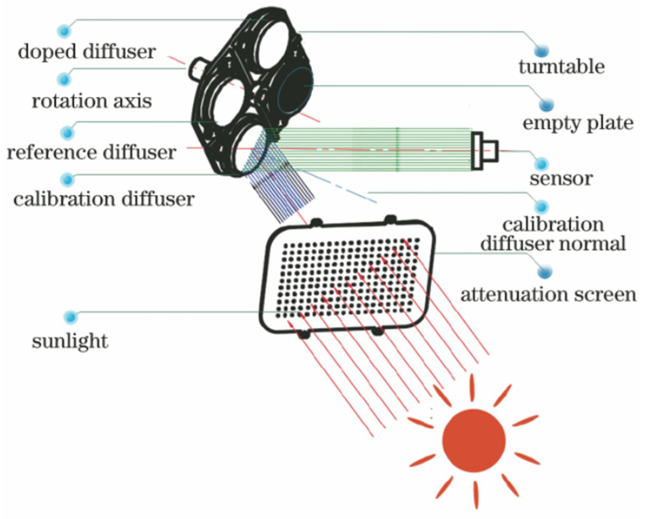
2.1.1. Onboard Absolute Calibration of SCS

The Satellite Calibration Spectrometer (SCS) is an imaging spectrometer designed for high-accuracy and high-frequency onboard cross-calibration for other instruments on the HY-1C satellite. The SCS is composed of two independent ultraviolet spectral channels and one visible and near-infrared spectral channel. The ultraviolet channel is designed for calibration of the ultraviolet imager (UVI), while the visible and near-infrared channels can be used for onboard calibration of the Chinese Ocean Color and Temperature Scanner (COCTS) and Coastal Zone Imager (CZI).

SCS uses a ±0.5° field of view (FOV) optical system combined with a coated line array detector (for ultraviolet channels) and an 11 × 100 pixels CCD (for visible and near-infrared channels) to achieve push-broom spectral imaging. The spectral imaging of the two ultraviolet channels is realized through two narrow-band filters coated on one line array detector, with continuous visible and near-infrared imaging realized using grating spectroscopy. SCS can achieve ±30° side swing imaging through the one-dimensional pointing mechanism, which can point to the set angle and stabilize according to the satellite’s instructions. In turn, the cross-calibration of the optional area or FOV between the sensors of HY-1C can be achieved. The spectral response range of the SCS is 400–900 nm, the spectral resolution is 5 nm and the field of view (FOV) is ±0.5°, corresponding to a swath width of 12 km. The nominal signal-to-noise ratio (SNR) of the SCS is better than 1000. The spatial resolution of the SCS at nadir is 1.1 km. It is designed the same as the spatial resolution of COCTS to improve the cross-calibration accuracy.

The SCS uses the Sun as the standard calibration source to achieve onboard radiometric calibration and obtain the absolute calibration coefficient of the sensor. The Sun is a highly stable and uniform Lambertian source. Since the solar constant and spectral irradiance distribution of the Sun outside the atmosphere change very little during a solar activity cycle, the Sun is an ideal onboard calibration source. Sun-based radiometric calibration is one of the most mainstream onboard calibration methods for remote sensors at present.

The operation mode and calibration period are shown in Figure 1. The arrow direction is the satellite flight direction. θ represents the incident angle of the sunlight to the calibration module. θ is restrained from 14.9° to 21.1° so that only sunlight in this incident angle range can enter the calibration module. Within this angle range, the influence of atmospheric transmission and scattering is very small so that the calibration accuracy can be guaranteed. In fact, to ensure the consistency of the calibration data and improve the calibration accuracy, all the in-orbit calibration processes are performed at a fixed incident angle of 18.5°.

The SCS onboard calibration system (Figure 2) [27] is composed of a calibration wheel and a solar attenuation screen for attenuating the incident light. The calibration wheel consists of a calibration solar diffuser (CSD) for daily radiometric calibration, reference solar diffuser (RSD) for CSD long-term spectral reflectance monitoring, erbium-doped diffuser for spectral calibration and empty plate for dark current acquisition. The radiometric calibration sequence starts with dark current acquisition with the calibration wheel rotating the empty plate to the front of the SCS, followed by radiometric calibration with the CSD, and ends with dark current acquisition again. The exposure time of the calibration diffuser is 20 s for each calibration. The CSD degradation monitoring sequence, executed approximately once a month, is realized by the sequential observation of the CSD and RSD by the SCS along one orbit. The spectral calibration sequence, executed once a month, is realized by the SCS sequential observation of the CSD and erbium-doped diffuser along one orbit.

The relationship between the input radiance L^SCS and the SCS output signals can be expressed as:

$$L^{SCS}=(D{N}^{SCS}-D{N}_{offset}^{SCS})·Gai{n}^{SCS}$$

(1)

where $D{N}_{offset}^{SCS}$ is the dark current and Gain^SCS is the radiometric calibration gain. The CSD reflected spectral radiance at the calibration time can be expressed as:

$$L_{SD}^b(t)=\frac{\tau ({\theta }_{at},{\phi }_{at};t)\cos ({\theta }_{SD}^{in})E_s^b}{d_{SD}^2}·f({\theta }_{SD}^{in},{\phi }_{SD}^{in};{\theta }_{SD}^{ob},{\phi }_{SD}^{ob};b,t)$$

(2)

where the SD subscript represents the calibration solar diffuser; ${\theta }_{at}$ and ${\phi }_{at}$ are the zenith and azimuth angles of the incident sunlight to the attenuation screen, respectively; $\tau ({\theta }_{at},{\phi }_{at};t)$ represents the attenuation screen transmittance; ${\theta }_{SD}^{in}$ and ${\phi }_{SD}^{in}$ are the solar zenith and azimuth angles, respectively; ${\theta }_{SD}^{ob}$ and ${\phi }_{SD}^{ob}$ are the observation zenith and azimuth angles of the SCS, respectively; and $f({\theta }_{SD}^{in},{\phi }_{SD}^{in};{\theta }_{SD}^{ob},{\phi }_{SD}^{ob};b,t)$ represents the bidirectional reflectance distribution function (BRDF) of the CSD corresponding to spectral band b at calibration time t. In addition, d is the relative Sun-to-Earth distance factor, t is the calibration time, b represents the spectral band and $E_s^b$ is the equivalent solar spectral irradiance corresponding to spectral band b of the SCS. This can be obtained by the convolution of the relative spectral response of SCS band b and the standard solar spectral irradiance:

$$E_S^b=\frac{{{\displaystyle \int }}^{\hspace{0.17em}}{R}^b(\lambda )E(\lambda )\mathrm{d}\lambda }{{{\displaystyle \int }}^{\hspace{0.17em}}{R}^b(\lambda )\mathrm{d}\lambda }$$

(3)

where $E(\lambda )$ is the solar irradiance and $R^b(\lambda )$ is the spectral response function corresponding to band b.

The BRDF of the CSD at the calibration time can be obtained from the BRDF calibrated in the laboratory before launch by:

$$f({\theta }_{SD}^{in},{\phi }_{SD}^{in};{\theta }_{SD}^{ob},{\phi }_{SD}^{ob};b,t)=H_{SD}^b(t)f_{lab}({\theta }_{SD}^{in},{\phi }_{SD}^{in};{\theta }_{SD}^{ob},{\phi }_{SD}^{ob};b)$$

(4)

where $H_{SD}^b(t)$ is the degradation factor of CSD monitored and measured using RSD, and $f_{lab}({\theta }_{SD}^{in},{\phi }_{SD}^{in};{\theta }_{SD}^{ob},{\phi }_{SD}^{ob};b)$ is the prelaunch BRDF of CSD calibrated in the laboratory.

The spectral radiance of CSD can be obtained via the above derivation and can be used for the accurate calibration and monitoring of SCS spectral responsivity. The absolute radiometric calibration coefficient of the SCS can be monitored continuously via this method to realize real-time calibration and improve the calibration accuracy of the SCS. The absolute radiometric calibration uncertainty of the SCS is shown in

Table 1. Relative standard deviations of eight spectral bands between SCS and COCTS.

Uncertainty Sources			Measurement Uncertainty
			Individual	Combined
CSD	CSD BRDF * measurement uncertainty	Light source stability	0.2%	0.84%
		Stray light	0.2%
		Incident light angle	0.2%
		Light source to diffuser distance	0.2%
		Light source aperture	0.2%
		Incident light intensity signal	0.3%
		Reflectance light intensity signal	0.5%
	Uniformity (Considering the attenuation screen)		0.4%	0.4%
	Mounting angle uncertainty		0.35%	0.35%
	Spectral transmittance uncertainty of the attenuation screen	Light source stability	0.2%	0.58%
		Stray light	0.2%
		Measurement mechanism repeatability	0.35%
		Measurement noise	0.1%
		Aperture dimension accuracy	0.2%
		Fringe vignetting	0.3%
Prelaunch calibration	Performance monitoring slice directional—hemispherical reflectance ratio measurement uncertainty		0.5%	0.5%
RSD	Incident light angle inconsistency		0.2%	0.54%
	Reflectance ratio measurement stability		0.5%
Solar spectral irradiance uncertainty			1%	1%
Spectral response function measurement uncertainty			0.5%	0.5%
Stray light and uncertain factors			1%	1%
Combined standard uncertainty			2.0%

* Bidirectional reflectance distribution function.

. As all the uncertainty sources are independent, the combined uncertainty is equal to the square root of the squares sum of the individual uncertainty source.

2.1.2. Cross-Calibration of HY-1C Sensors

For general intersatellite cross-calibration, the accuracy is determined by observation factors such as the solar illumination angle, observation angle, atmospheric stability, uniformity of the observation target, image matching error and radiometric calibration error of the sensor. However, due to the orbital changes of different satellites, it is difficult for these observation factors to be completely consistent, so it is difficult to achieve very high intersatellite cross-calibration accuracy and to increase the calibration frequency.

The SCS uses the Sun as the standard radiometric calibration source for radiometric calibration and monitoring. The SCS can then be used as a transfer reference to calibrate the COCTS, CZI and UVI instruments mounted on the HY-1C satellite through the cross-calibration method. The TOA radiance can be used to calibrate the SCS, COCTS, UVI and CZI because (1) the four instruments are all mounted on the same platform, so strict time synchronization can be achieved. The imaging time difference is in the order of seconds, and it is much higher than the minute-level time synchronization of conventional intersatellite cross-calibration. (2) The relative position of each sensor and the optical axis orientation of each sensor are fixed and measured precisely before launch, so an accurate pixel matching model between the SCS and the other three instruments can be acquired after the initial onboard geometric calibration.

For the four sensors mounted on HY-1C or other sensors with the same observation geometry and similar transit time within two hours, the technical route of cross-calibration using SCS is the same as the standard cross-calibration process of COCTS shown in Figure 3.

More detailed information about the cross-calibration and validation of SCS and other sensors of HY-1C can be found in [27,28,29,30].

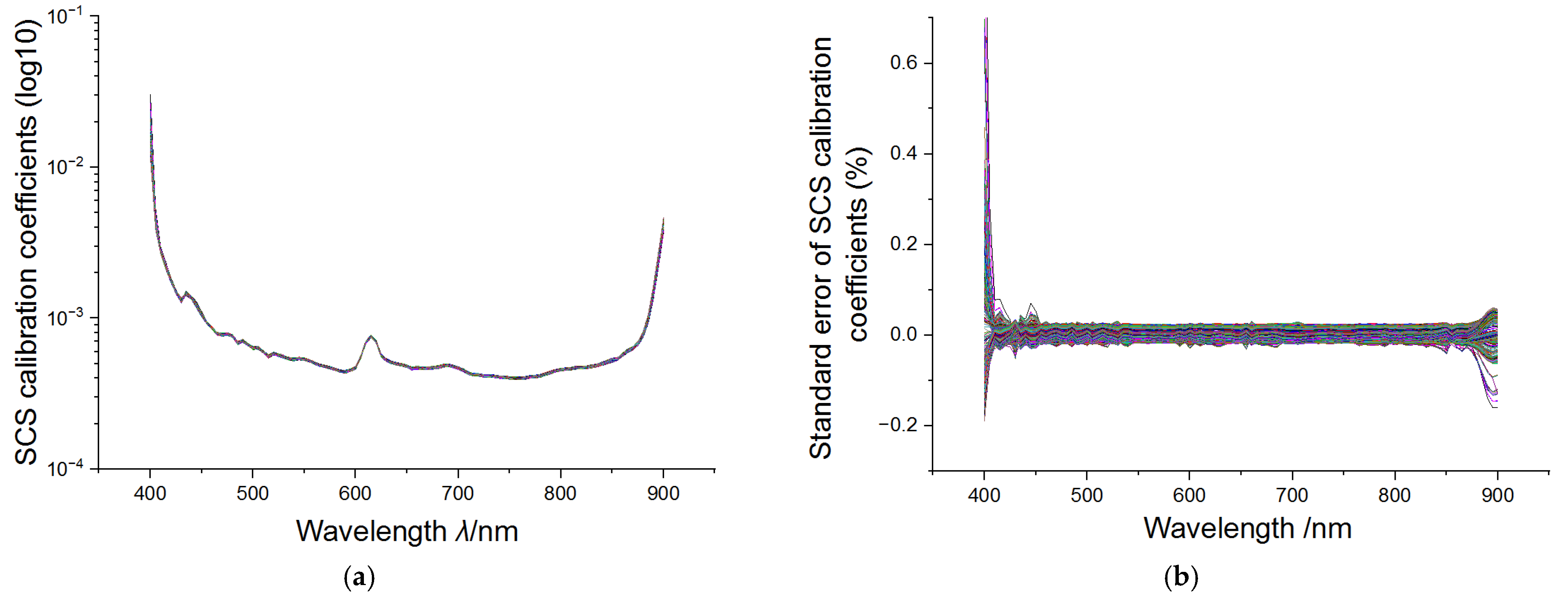
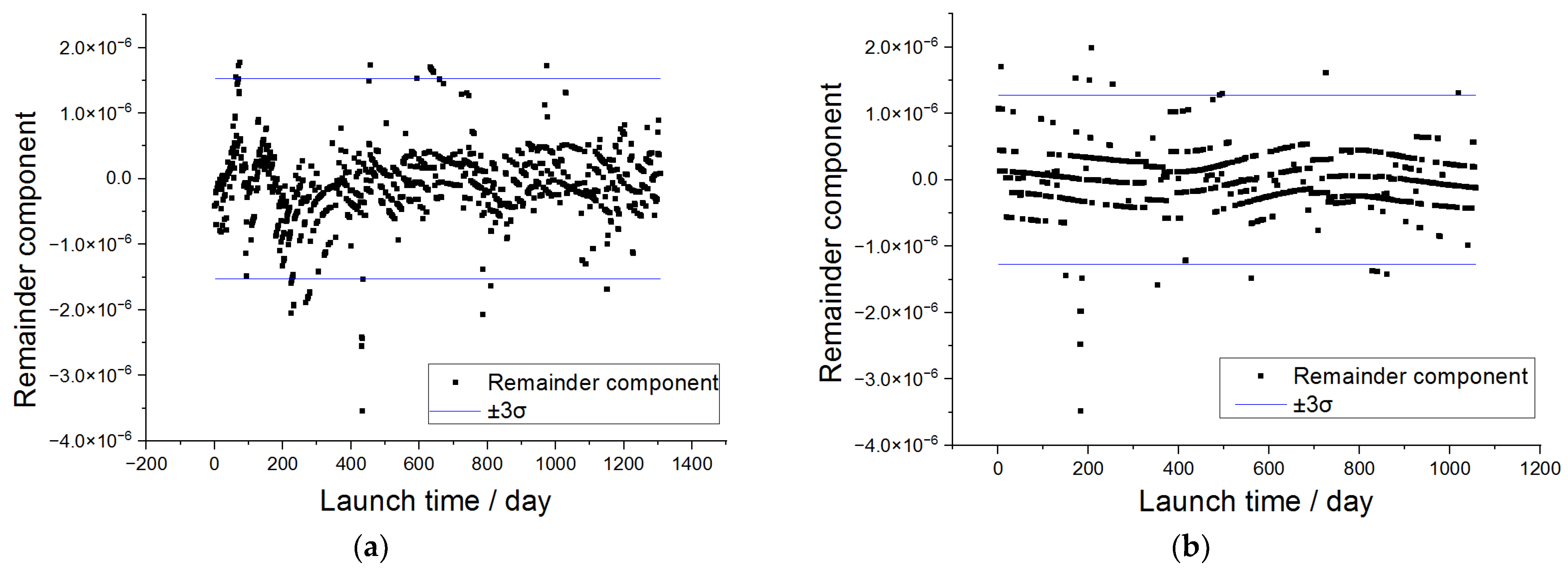
2.2. Long-Term Calibration Coefficients of SCS and Data Preprocessing

The above-described calibration observation physical model represents our best knowledge of the SCS instrument, onboard calibration module and Sun-based absolute radiometric calibration process. The SCS onboard calibration coefficient of 65 ms integration time and 1 gain over all visible and near infrared spectral bands is shown in Figure 4. The SCS calibration coefficients of most spectral bands vary little (less than 5%) and they show satisfactory stability.

The long-term calibration coefficient changes in each spectral band over time are quite similar. Figure 5 shows the long-term calibration coefficients of five different spectral bands of the SCS, and they share a very similar changing regularity. This is studied in the following sections.

Ideally, the onboard calibration error caused by such factors can be eliminated through the above model and data processing. However, in practice, the corrected calibration coefficient using the above observation model always retains some errors that can hardly be defined as random from the perspective of statistics. Here, a time series analysis-based method is performed on the long-term SCS onboard calibration data to analyze and correct the calibration coefficients.

Before May 2019, the SCS is in the state of testing, and its calibration frequency is not stable. From 1 May 2019 to 1 January 2020, the SCS is calibrated every two days using CSD; and from 1 January 2020 to the present, the SCS is calibrated every day using CSD. The spectral calibration and long-term spectral response change calibration using RSD were performed every two months. Figure 6a shows the original onboard calibration coefficient time series of the 19th visible spectral band (central wavelength 490 nm) of SCS from launch day 8 September 2018 to 7 April 2022. These calibration coefficient time series data were corrected using the RSD calibration method, and the effect of the Sun to SCS distance on solar irradiance has also been eliminated according to Equation (2).

Therefore, the calibration frequency over the entire calibration coefficient time series is inconsistent. For the time series analysis method, the original calibration coefficient data must be preprocessed to a standard time series data format. The repetitive data are eliminated and the scarce calibration data are added through linear interpolation. The original data are interpolated according to launch day, with the time series frequency set to 365.25 days according to the period of the Earth’s revolution. The processed calibration coefficient time series is shown in Figure 6b.

Note that the SCS calibration coefficient in the first 250 days is scarce due to the low calibration frequency. Linear interpolation is performed to complete the scarce data, but too many interpolated values may break the potential statistical characteristics of the calibration coefficient data. To study the effect of the scarce data, the original calibration coefficient data and the data without the first 250 days (Figure 6c) are modeled.

The fluctuation in the calibration coefficients is less than ±2.3% (ratio of the peak-valley and the average value). It can also be easily seen that the SCS calibration coefficient has an obvious regularity: there is a very small degradation trend, an obvious periodic change and a certain high-frequency noise in the calibration coefficient time series. The autocorrelation test of the data shown in Figure 6a is performed, with the result shown in Figure 7. The result shows a strong autocorrelation, and the SCS onboard calibration coefficients are obviously not a random series, indicating that there are some system errors that have not been corrected.

The residual system errors may be caused by the orbit position deviation, temperature drift of the satellite and the sensor, installation angle deviation of the sensor and the CSD or other factors. Efforts have been made to control and correct these error factors in the prelaunch calibration process in the laboratory, but some residual errors remain, and the influence of these errors cannot be determined and corrected by accurate physical models after the sensor is launched. Therefore, we want to separate and eliminate the influence of residual system error from the perspective of statistics using the methods of time series analysis.

2.3. Time Series Modeling and Analysis Method

The long-term onboard calibration coefficient data of remote sensors are typical time series data, and further information about the sensor can be obtained by analyzing the calibration coefficient time series. The commonly used time series analysis methods include classical linear and nonlinear analysis methods such as the autoregressive moving average model (ARMA) [30], with time series analysis methods based on machine learning such as the recurrent neural network (RNN) [31,32] and long–short time memory network (LSTM) [33]. In this paper, a classical time series modeling method of STL (seasonal and trend decomposition using loess) [34] and a machine learning-based method of long short-term memory (LSTM) neural network are used to model and analyze the radiometric calibration coefficient, respectively.

2.3.1. Seasonal and Trend Decomposition Using Loess

Seasonal and trend decomposition using loess (STL) is a time series decomposition method based on the locally weighted scatterplot smoothing LOWESS or LOESS (LOESS) method. Loess is a local polynomial regression fitting method that is a common method for smoothing two-dimensional scatterplots. It combines the simplicity of traditional linear regression and the flexibility of nonlinear regression. When estimating the value of a response variable, a data subset from the vicinity of its predictor variable is taken, a regression or quadratic regression on the subset is performed and the weighted least squares method is used for regression. A value closer to the estimated point has a greater weight. Finally, the obtained local regression model can be used to estimate the response variable value. This method performs point-by-point operations to obtain the entire fitted curve. STL is robust to outliers by using the robust LOESS [35] and can only handle additive mode decomposition. The STL method also has a weakness in that it cannot distinguish the seasonal component and the periodic component accurately; thus, it is not suitable for complex time series decomposition and forecasting.

Compared with various complex time series data such as finance and hydrology, there are far fewer factors that may affect the onboard radiometric calibration coefficient, and most of them can be accurately identified and modeled physically. An obvious advantage of STL is that its decomposition method has much better interpretability: the trend component can be explained as the long-term degradation of the onboard calibration module and SCS instrument; the seasonal or periodic component can be explained as the periodic orbital position change of the sensor (there are almost no other periodic influencing factors for in-orbit remote sensors); and the remainder noise represents the random measurement error of the sensor and the calibration module. All three influencing factors conform to the additive mode of the total calibration uncertainty. Therefore, the STL decomposition model can also be verified by the statistical relationship between the physical model and the data-driven model.

For these reasons, the concise and explicable STL method is chosen as the time series decomposition method to model and analyze the SCS calibration coefficients.

2.3.2. Long Short-Term Memory (LSTM) Neural Network

Machine learning technology is widely used for time series modeling. Generally, machine learning-based methods are very suitable for processing large amounts of multidimensional data with complex structures and always have better modeling accuracy than classical time series methods. However, the interpretability of machine learning models is always poor. Therefore, the machine learning method-based model can only be used to fit and forecast time series data.

Compared with other complex algorithms such as dendritic neural regression (DNR) [36] and graph neural networks (GNN) [37], which are designed for more complex data analysis tasks, LSTM has sufficient modeling accuracy and lower complexity. Therefore, we use an LSTM neural network to model the SCS calibration coefficient time series.

LSTM is a modified RNN that is designed to solve the problem of gradient vanishing and explosion during long-sequence data training. LSTM is based on a simple RNN and adds some multithreshold gates to solve the storage and forgetting problems. Therefore, LSTM can deal with long-term dependency problems. LSTM is regarded as one of the most effective methods to deal with the problem of time series prediction, so we use LSTM as a typical example of machine learning-based time series modeling methods to evaluate their performance.

3. Results

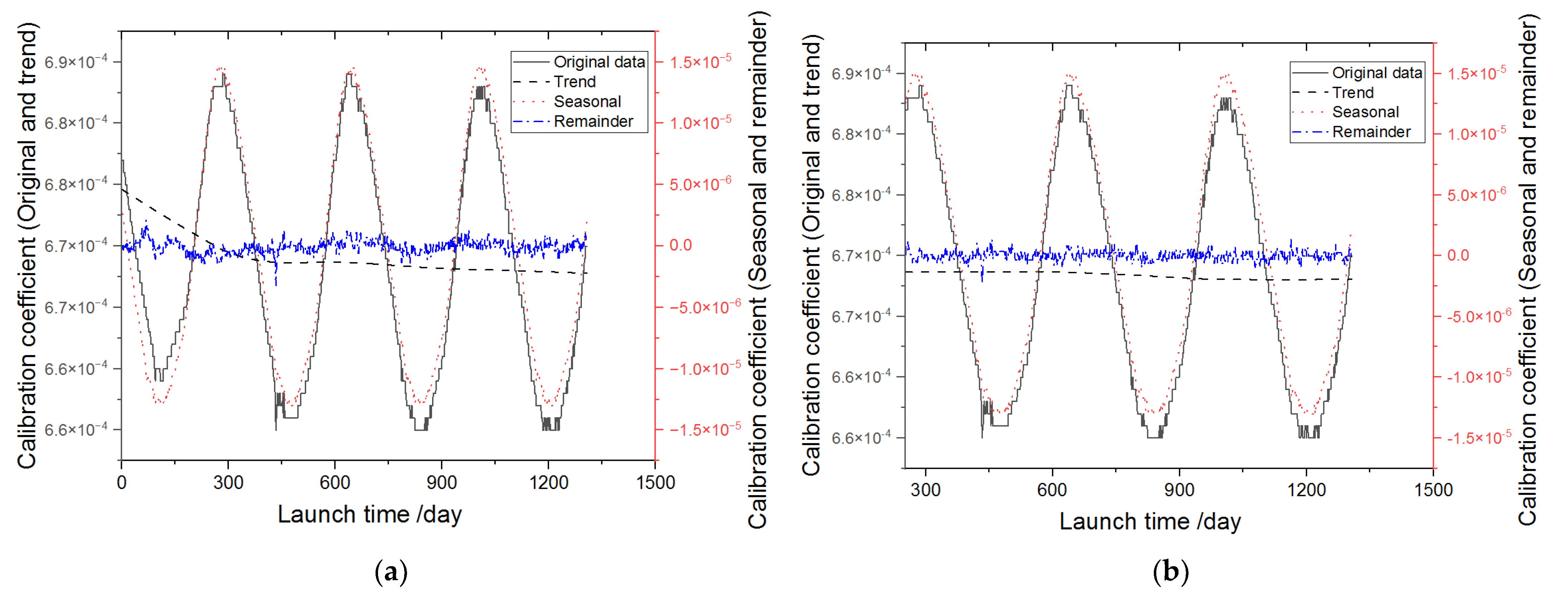
3.1. STL-Based SCS Calibration Coefficient Modeling and Analysis

3.1.1. STL Modeling Results

Based on the STL decomposition method, the calibration coefficient time series Coef can be decomposed into a trend component, seasonal component and remainder component:

$$Coef=T_c+S_c+R_c$$

(5)

where T_c, S_c and R_c represent the trend, seasonal and remainder components, respectively.

Figure 8 shows the STL decomposition results of the SCS calibration coefficient data in Figure 6b,c. The trend, seasonal and remainder components are obtained. The remaining components show much higher randomness compared with that of the original calibration coefficient data. Thus, both decomposition results can be considered effective, but the difference between the two decomposition results should be considered and discussed.

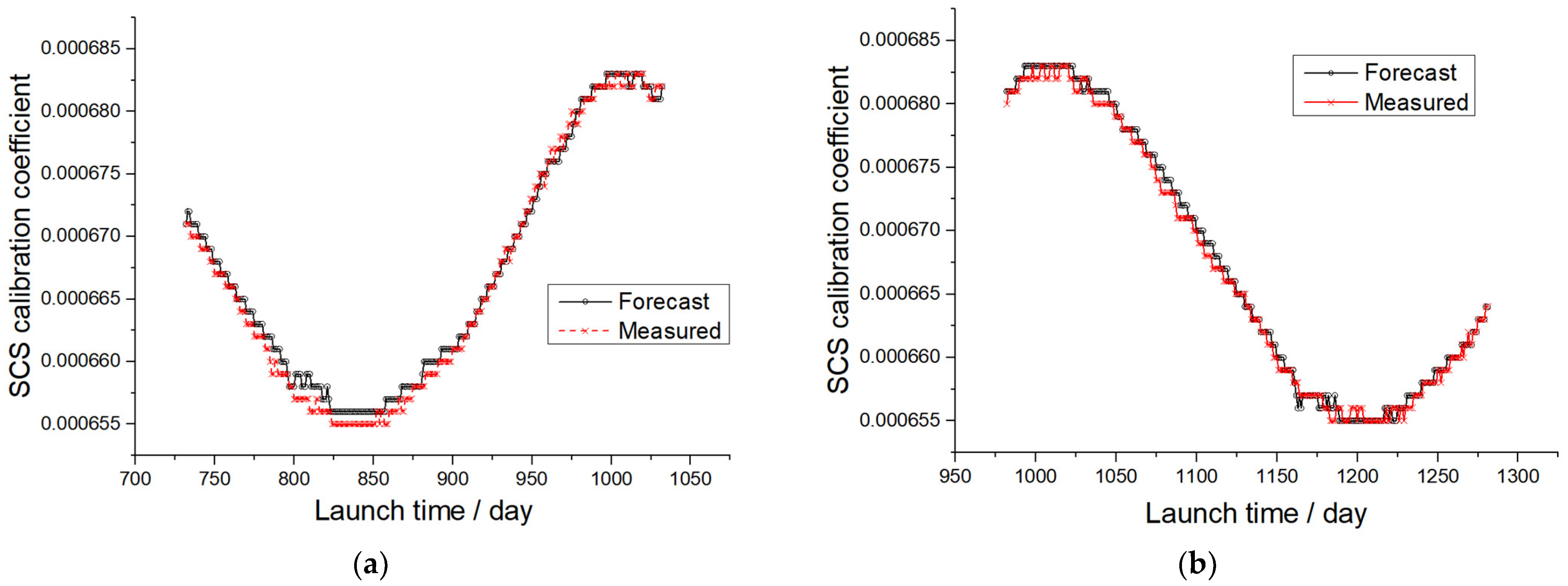
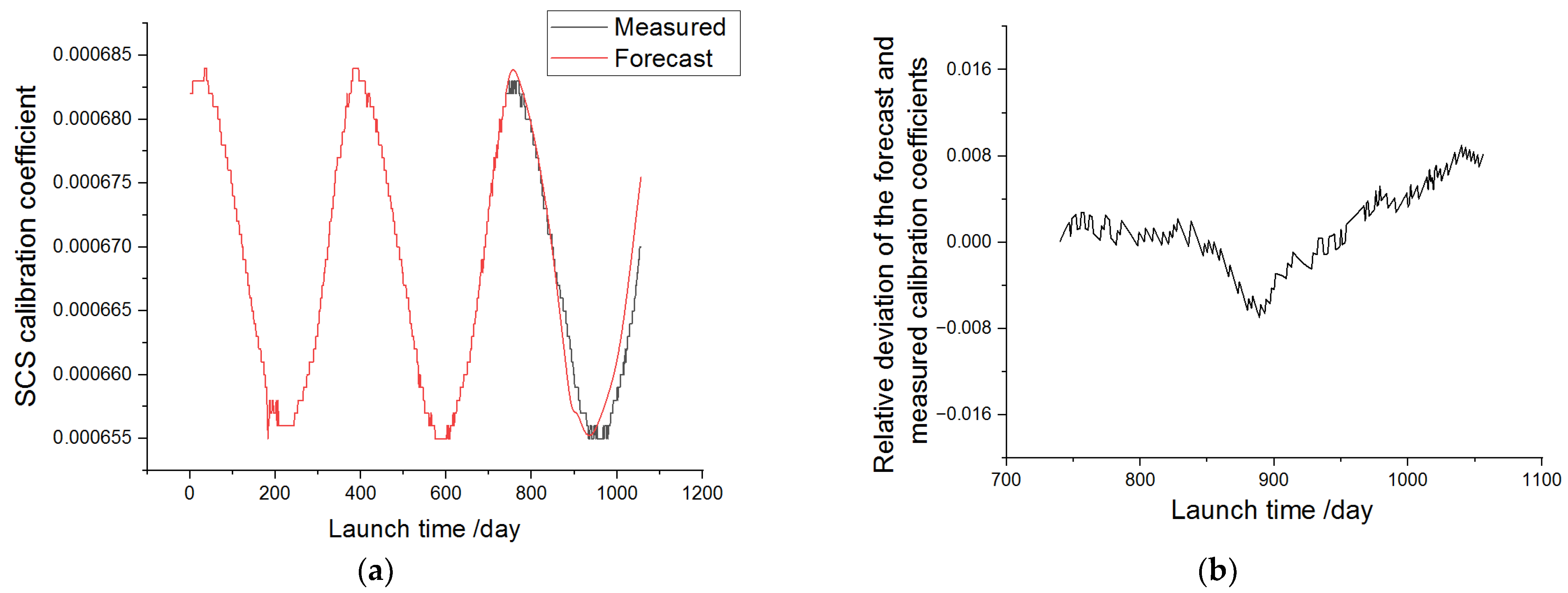
3.1.2. Forecast, Validation and Correction of Calibration Coefficients Using STL Model

The time series model is constructed based on the long-term performance of the SCS instrument and can represent its inherent response changing pattern. Therefore, the calibration coefficient can be predicted, verified and corrected using the constructed time series model, which can also help correct the SCS onboard calibration coefficients.

• Calibration coefficient forecast

Data forecasting is one of the most common applications of time series analysis. The first 730 data in Figure 6b,c are used for the STL training dataset, with the following 300 data used as the forecast accuracy validation dataset. The comparisons between the forecast and measured data and their relative deviation are shown in Figure 9. Figure 10 shows the 80% and 95% probability intervals of the forecast calibration coefficients. As can be seen, the forecast accuracy and dispersion range using the data without the first 250 days are both better than those using the original complete data, which indicates a higher reliability of the model and forecast coefficients.

2.

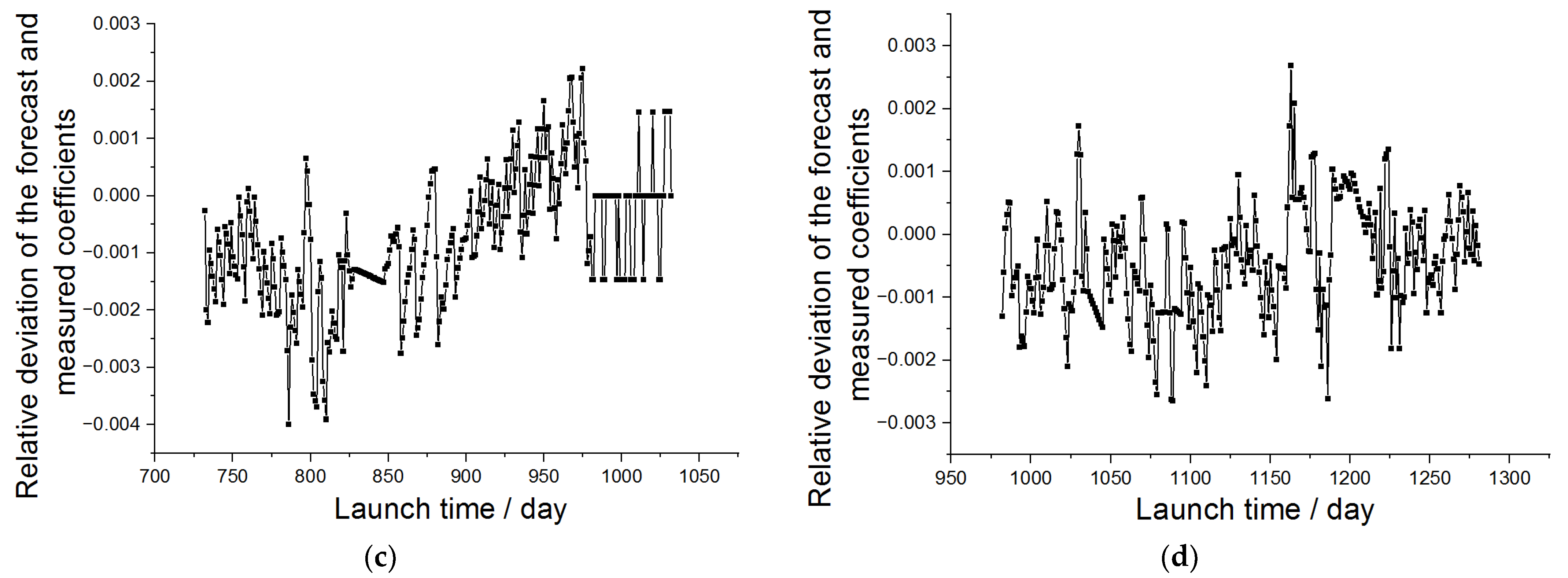
Anomaly calibration coefficient detection

The time series model can also be used to determine outliers. Assuming the remainder conform to the Gaussian distribution, the 3σ criterion can be used to search for outliers. Figure 11 shows the remaining components and their corresponding 3σ criterion lines. Outliers can be found and eliminated according to this.

3.

Calibration coefficient correction

According to the above analysis, we believe that the relatively large trend component shown in Figure 8a is caused by the incomplete calibration coefficients in the first 250 days and is not reliable. Therefore, the time series model without the first 250 days of data is used to correct the SCS calibration coefficients. As discussed above, the seasonal components that represent the main residual errors and the outlier data should be eliminated. The corrected calibration coefficient without the first 250 days is shown in Figure 12.

The degradation trend of the corrected calibration coefficients is about 4.8 × 10⁻⁴ and can be treated as a constant. This verifies the effectiveness of the designed onboard calibration and monitoring method of SCS. The standard deviation of the corrected calibration coefficients is 8 × 10⁻⁴. This result conforms to the designed SNR level of the SCS and can verify the effectiveness of the proposed calibration coefficient correctness method.

3.2. LSTM-Based SCS Calibration Coefficient Modeling and Analysis

According to the principle of machine learning, the trained LSTM model is a black box for users, and it can hardly be understood or interpreted. Therefore, we can only test the performance of the LSTM model by evaluating its forecast accuracy. The LSTM network is trained for 700 iterations, the learning rate is set to 0.01 and the loss function is the root mean square of the model error. The first 730 data in Figure 6c are used as the training dataset and the following 300 data are used as the validation dataset. The loss function appears to be constant during the last 100 training loops, indicating that the LSTM model reached its best performance.

The forecast accuracy using the constructed LSTM model is shown in Figure 13a. The comparisons between the forecast and the measured data and their relative deviation are shown in Figure 13b. The forecast accuracy using LSTM is approximately 3.5 × 10⁻³ and is worse than the forecast accuracy using the STL method.

4. Discussion

4.1. Discussion of the STL Decomposition Results

Based on the time series decomposition results described above, some information of the SCS onboard calibration coefficient can be acquired. The decomposed components are discussed as follows.

4.1.1. Trend Component

For the trend component, in Figure 8a, there is an obvious degradation trend of the original time series, and the trend can be explained by the sensor or the calibration module change over time. However, it can also be noticed that the trend slope of the first 250 days is much steeper than that of the last data, which is abnormal in nature. For the trend component of the data without the first 250 days, its fluctuation amplitude is three orders of magnitude smaller than the seasonal and remainder components; thus, it can be treated as a constant that represents the average onboard calibration coefficient over in-orbit operation time.

As described above, in-orbit calibration using RSD is performed every two months to correct the long-term change in the CSD and SCS. Thus, the long-term calibration coefficient degradation should be relatively stable. Therefore, comparing the two trend components shown in Figure 8, we believe that the slope deviation of different period time series is caused by the insufficient calibration coefficient data in the first 250 days, with the time series model shown in Figure 8b more accurate. This can also be proven by the remaining autocorrelation coefficient and the calibration coefficient forecast accuracy described in the following sections.

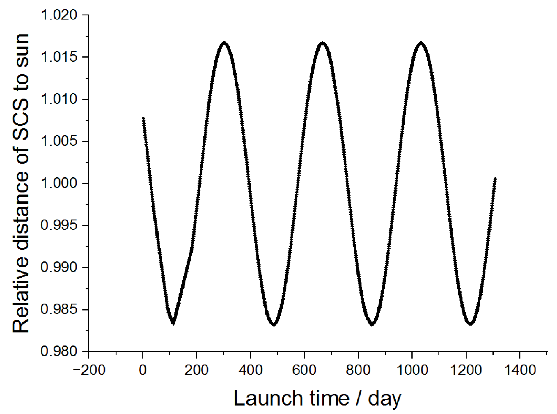
4.1.2. Seasonal Component

The seasonal component shown in Figure 8 is quite significant. As mentioned above, the seasonal component is considered to be closely related to the sensor’s orbital position change over the years, so a correlation analysis is performed to verify this. We use the Sun-to-SCS distance provided by the HY-1C telemetry data as the representation of the SCS orbital position, which is shown in Figure 14, with the Pearson correlation coefficient used to evaluate the correlation of the seasonal component and the Sun-to-SCS distance:

$$Corcoef=\frac{\mathrm{Cov}(s2s, seasonal)}{\mathsf{\sigma }(e2s)·\mathsf{\sigma }(seasonal)}$$

(6)

where Corcoef represents the Pearson correlation coefficient, s2s represents the distance between the Sun and SCS, seasonal is the decomposed seasonal component, Cov is the covariance calculation and $\sigma$ represents the standard deviation calculation.

The obtained Pearson coefficients are 0.975, which indicate a very strong correlation between the SCS orbital position and the onboard calibration coefficient. Therefore, according to the physical error factor analysis and the data analysis results, we believe that the residual periodic error represented by the seasonal component could be caused by factors such as orbital position error, Sun-orientation error of CSD/RSD and other factors that are closely related to the Sun–SCS distance. As it is caused by residual system errors, the seasonal component should be eliminated to improve the SCS onboard calibration accuracy.

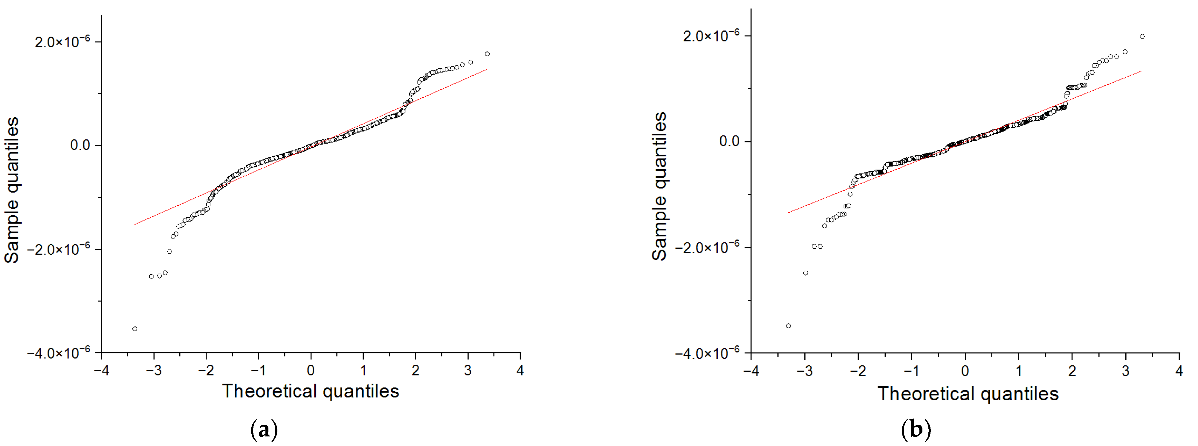
4.1.3. Remainder Component

Theoretically, if all system errors are separated and eliminated in the trend and seasonal components, then the remainder component should be approximately white noise. The degree of randomness of the remainder component is an important evaluation criterion for the model correctness; more randomness always means that more pattern information of the original data has been extracted. Here, we use the Ljung–Box test, quantile–quantile plots and autocorrelation (ACF)/partial autocorrelation (Partial ACF) to evaluate the randomness of the remainder component and verify the effectiveness of the STL decomposition results.

The p values for the Ljung–Box tests of the remaining components of the data shown in Figure 6b,c are both close to 0. They are both less than the significance level of 0.05; thus, they are not random series. The quantile–quantile plots and the autocorrelation/partial autocorrelation of the remainder component of the data shown in Figure 6b,c are shown in Figure 15 and Figure 16, respectively. From these test results, we can also see that the remaining components of the two sets of data are not random series.

Compared with the autocorrelation of the original calibration coefficient shown in Figure 7, the autocorrelation of the remaining components in Figure 16 shows a much higher randomness. The relative standard deviation of the remaining components is approximately 8 × 10⁻⁴, which conforms to the SCS nominal SNR level of approximately 1000. This verifies the effectiveness of the STL decomposition results from another point of view.

Comparing the two autocorrelation results in Figure 16a,c, the remainder components are both within the two-time standard deviation range when the time lag is relatively long. The remainder component of the time series without the first 250 days of data shows a lower autocorrelation, which also indicates that the corresponding model decomposition result has higher reliability.

In fact, we have tried other time series modeling methods such as autoregressive integrated moving average (ARIMA) [38], which can obtain higher data fitting accuracy with more random residual errors. However, we still believe that the STL model works better for the calibration coefficient data correction task. First, the relative deviation of the STL model remainder component can conform to the nominal SNR of SCS, and lower levels of error of the ARIMA residual component indicate overfitting and are hard to physically explain. Second, the interpretability of the ARIMA method is poorer, with the trend and seasonal components eliminated during the difference process, making it difficult to be physically explained. Finally, the ARIMA model cannot be physically explained and tested, so its reliability is also questionable.

4.1.4. Correlation of Different Spectral Band Calibration Coefficients

Pearson coefficients between the calibration coefficients of different spectral bands shown in Figure 5 are obtained to evaluate the degree of correlation and infer the calibration error source. The Pearson coefficients are listed in

Table 2. Pearson correlation coefficients of Sun-to-SCS distance s2s and 16th, 32nd, 48th, 64th and 80th spectral bands of SCS.

	16th	32nd	48th	64th	80th	s2s
16th	-	0.999	0.990	0.997	0.993	0.973
32nd	0.999	-	0.993	0.999	0.996	0.974
48th	0.990	0.993	-	0.995	0.998	0.974
64th	0.997	0.999	0.995	-	0.997	0.972
80th	0.993	0.996	0.998	0.997	-	0.971

. The degrees of correlation between different spectral bands are all nearly 1, which indicates that the calibration coefficient fluctuations are likely caused by the same influencing factors. STL decomposition is performed on each spectral band calibration coefficient, with decomposition results similar to those in Figure 8 obtained. Combined with the correlation analysis of the Sun-to-SCS distance and the calibration coefficient described above, we believe that all SCS calibration coefficient fluctuations are caused by some uncertain error factors that are closely related to the SCS orbital position change over time. Due to the high consistency of the calibration coefficients of each spectral band, only one representative spectral band calibration coefficient needs to be modeled and analyzed.

4.2. Discussion of the LSTM-Based SCS Calibration Coefficient Modeling and Analysis

As shown in Figure 13, the forecast accuracy of LSTM is worse than that of using the STL method. The reason is that the time series data structure is simple and the data size is small, so the advantages of the machine learning method are not obvious. Moreover, the trained model can hardly be understood and interpreted; therefore, the LSTM model cannot be used for calibration error separation and correction. The reliability of the LSTM model is also poor for the same reason. These problems are caused by the inherent deficiency of existing machine learning technology, and there are currently no solutions to improve this issue.

5. Conclusions

The onboard calibration accuracy of remote sensors is crucial for quantitative ocean remote sensing applications, with the onboard calibration method using the onboard calibration module one of the most effective and accurate methods to guarantee the accuracy of remote sensing measurement. The Satellite Calibration Spectrometer is a calibration imaging spectrometer designed for cross-calibration for other sensors mounted on the HY-1C satellite. Although most onboard calibration errors using the onboard calibration module can be corrected based on the observation physical model and the prelaunch radiometric and observation geometry calibration, the calibration coefficients of the SCS retain some regularity, which indicates the existence of residual calibration errors. In this case, the observation physical model cannot help reduce the residual error.

Therefore, data analysis-based methods were proposed in this study to solve this problem. First, the onboard calibration method and long-term calibration coefficients of the SCS were described, then the STL and LSTM methods were used to model and analyze the SCS calibration coefficients. Finally, the constructed time series models were used to forecast, validate and correct the calibration coefficients in order to verify the effectiveness of these methods.

The analysis results show that the STL method is effective for modeling and correcting the SCS onboard calibration coefficient time series because of its good interpretability. Each decomposition component of the STL model can correspond to the physical factors in the calibration physical process from a statistical perspective, and the combination of knowledge-driven and data-driven models can help demonstrate the rationality and effectiveness of this method. The data fitting and forecast accuracy of the STL method are also satisfactory.

However, there remain some points to be considered: 1. The calibration coefficient time series of different sensors always have different characteristics; thus, different time series analysis methods should be further analyzed for a wider range of applications. 2. We have only tested the constructed STL model via statistical methods, with the verification of the physical significance corresponding to the STL model components still insufficient.

For machine-learning-based time series analysis methods such as LSTM, model interpretability is a large obstacle to application. The trained model is a black box for us and can provide no information about the sensor calibration process except for accurate fitting and forecasting of the input data; the model reliability is poor for the same reason. Therefore, although the forecast accuracy of LSTM is also acceptable, we believe that machine-learning-based methods are not suitable for the correction of calibration coefficients.

In summary, we proposed to apply time series analysis methods to the correction of remote sensor onboard calibration coefficients, with the statistical analysis results demonstrating the effectiveness of the proposed methods. We believe that the proposed data-driven analysis methods can supply additional reference information for sensor operation status monitoring and help improve the in-orbit calibration accuracy of remote sensors.

References

1. Lewis, K.M.; Arrigo, K.R. Ocean color algorithms for estimating chlorophyll a, CDOM absorption, and particle backscattering in the Arctic Ocean. J. Geophys. Res. Oceans 2020, 125, e2019JC015706. [Google Scholar] [CrossRef]
2. Tassan, S.; Sturm, R. An algorithm for the retrieval of sediment content in turbid coastal waters from CZCS data. Int. J. Remote Sens. 1986, 7, 643–655. [Google Scholar] [CrossRef]
3. Ahn, Y.H.; Shanmugam, P. Detecting the red tide algal blooms from satellite ocean color observations in optically complex Northeast-Asia Coastal waters. Remote Sens. Environ. 2006, 103, 419–437. [Google Scholar] [CrossRef]
4. Miguel, A.; Santos, P. Fisheries oceanography using satellite and arborne remote sensing methods: A review. Fish. Res. 2000, 49, 1–20. [Google Scholar]
5. Waite, J.N.; Mueter, F.J. Spatial and temporal variability of chlorophyll-a concentrations in the coastal Gulf of Alaska, 1998–2011, using cloud-free reconstructions of SeaWiFS and MODIS-Aqua data. Prog. Oceanogr. 2013, 116, 179–192. [Google Scholar] [CrossRef]
6. Frouin, R. In-Flight Calibration of Satellite Ocean-Colour Sensors. In Reports of the International Ocean-Colour Coordinating Group No. 14; IOCCG: Dartmouth, NS, Canada, 2013. [Google Scholar]
7. Eplee, R.E.; Turpie, K.R.; Fireman, G.F.; Meister, G.; Stone, T.C.; Frederick, S.P.; Franz, B.A.; Bailey, S.W.; Robinson, W.D.; McClain, C.R. VIIRS on-orbit calibration for ocean color data processing. In Proceedings of the SPIE 8510, Earth Observing Systems XVII, San Diego, CA, USA, 15 October 2012. [Google Scholar]
8. Mélin, F.; Zibordi, G. Vicarious calibration of satellite ocean color sensors at two coastal sites. Appl. Opt. 2010, 49, 798–810. [Google Scholar] [CrossRef]
9. Xiong, X.; Wu, A.; Wenny, B.N.; Madhavan, S.; Wang, Z.; Li, Y.; Chen, N.; Barnes, W.L.; Salomonson, V.V. Terra and Aqua MODIS Thermal Emissive Bands in-orbit Calibration and Performance. IEEE Trans. Geosci. Remote Sens. 2015, 53, 5709–5721. [Google Scholar] [CrossRef]
10. Cao, C.; de Luccia, F.J.; Xiong, X.; Wolfe, R.; Weng, F. Early in-orbit performance of the Visible Infrared Imaging Radiometer Suite onboard the Suomi National Polar-Orbiting Partnership (S-NPP) satellite. IEEE Trans. Geosci. Remote Sens. 2014, 52, 1142–1156. [Google Scholar] [CrossRef]
11. Clark, D.; Feinholz, M.; Yarbrough, M.; Johnson, B.; Brown, S.; Kim, Y.; Barnes, R. Overview of the radiometric calibration of MOBY. In Proceedings of the SPIE 4483, Earth Observing Systems VI, San Diengo, CA, USA, 18 January 2002. [Google Scholar]
12. Sun, J.; Wang, M. Radiometric calibration of the Visible Infrared Imaging Radiometer Suite reflective solar bands with robust characterizations and hybrid calibration coefficients. Appl. Opt. 2015, 54, 9331–9342. [Google Scholar] [CrossRef]
13. Sun, J.; Xiong, X.; Barnes, W. MODIS solar diffuser stability monitor sun view modeling. IEEE Trans. Geosci. Remote Sens. 2005, 43, 1845–1854. [Google Scholar]
14. Xiong, X.; Sun, J.; Barnes, W.; Salomonson, V.; Esposito, J.; Erives, H.; Guenther, B. Multiyear in-orbit Calibration and Performance of Terra MODIS Reflective Solar Bands. IEEE Trans. Geosci. Remote Sens. 2007, 45, 879–889. [Google Scholar] [CrossRef]
15. Meister, G.; Pattb, F.S.; Xiong, X.; Sun, J.; Xie, X.; McClain, C.R. Residual correlations in the solar diffuser measurements of the MODIS Aqua ocean color bands to the sun yaw angle. In Proceedings of the SPIE 5882, Earth Observing Systems X, Bellingham, WA, USA, 31 July 2005. [Google Scholar]
16. Meister, G.; Sun, J.; Eplee, R.E., Jr.; Pattc, F.S.; Xiong, X.; McClain, C.R. Sun beta angle residuals in solar diffuser measurements of the MODIS ocean bands. In Proceedings of the SPIE 7081, Earth Observing Systems XIII, San Diengo, CA, USA, 10 August 2008. [Google Scholar]
17. Xiong, X.; Angal, A.; Choi, T.; Sun, J.; Johnson, E. In-orbit Performance of MODIS Solar Diffuser Stability Monitor. In Proceedings of the SPIE 8510, Earth Observing Systems XVII, San Diengo, CA, USA, 10 August 2008. [Google Scholar]
18. Eplee, R.E.; Meister, G.; Patt, F.S.; Barnes, R.A.; Bailey, S.W.; Franz, B.A.; McClain, C.R. In-orbit calibration of SeaWiFS. Appl. Opt. 2012, 51, 8702–8730. [Google Scholar] [CrossRef] [PubMed]
19. Eplee, R.E., Jr.; Meister, G.; Patt, F.S.; McClain, C.R. The in-orbit Calibration of SeaWiFS: Functional Fits to the Lunar Time Series. In Proceedings of the SPIE 7081, Earth Observing Systems XIII, San Diengo, CA, USA, 10 August 2008. [Google Scholar]
20. Bisoi, R.; Dash, P.K.; Parida, A.K. Hybrid Variational Mode Decomposition and evolutionary robus kernel extreme learning machine for stock price and movement prediction on daily basis. Appl. Soft Comput. 2018, 74, 652–678. [Google Scholar] [CrossRef]
21. Eymen, A.; Köylü, U. Seasonal trend analysis and ARIMA modeling of relative humidity and wind speed time series around Yamula Dam. Meteorol. Atmos. Phys. 2019, 131, 601–612. [Google Scholar] [CrossRef]
22. Sang, Y. A review on the applications of wavelet transform in hydrology time series analysis. Atmos. Res. 2013, 122, 8–15. [Google Scholar] [CrossRef]
23. Li, R.; Jiang, P.; Yang, H.; Li, C. A novel hybrid forecasting scheme for electricity demand time series. Sustain. Cities Soc. 2020, 55, 102036. [Google Scholar] [CrossRef]
24. Schmidt, M.; King, E.A.; Mcvicar, T.R. A method for operational calibration of AVHRR reflective time series data. Remote Sens. Environ. 2008, 112, 1117–1129. [Google Scholar] [CrossRef]
25. Saadi, S.; Simonneaux, V.; Boulet, G.; Raimbault, B.; Mougenot, B.; Fanise, P.; Ayari, H.; Lili-Chabaane, Z. Monitoring Irrigation Consumption Using High Resolution NDVI Image Time Series: Calibration and Validation in the Kairouan Plain (Tunisia). Remote Sens. 2015, 7, 13005–13028. [Google Scholar] [CrossRef]
26. Campbell, P.K.E.; Middleton, E.M.; Thome, K.J.; Kokaly, R.F. Eo-1 hyperion reflectance time series at calibration and validation sites: Stability and sensitivity to seasonal dynamics. IEEE J. Sel. Top. Appl. Earth Obs. Remote Sens. 2013, 6, 276–290. [Google Scholar] [CrossRef]
27. Xu, H.; Zhang, L.; Huang, W.; Li, X.; Si, X.; Xu, W.; Song, Q. On-board Absolute Radiometric Calibration and Validation Based on Solar Diffuser of HY-1C SCS. Acta Optica. Sin. 2020, 40, 181–190. [Google Scholar]
28. Xu, H.; Zhang, L.; Huang, W.; Xu, W.; Si, X.; Chen, H.; Li, X.; Song, Q. Onboard absolute radiometric calibration and validation of the satellite calibration spectrometer on HY-1C. Opt. Express 2020, 28, 30015–30034. [Google Scholar] [CrossRef] [PubMed]
29. Song, Q.; Chen, S.; Xue, C.; Lin, M.; Huang, X. Vicarious calibration of COCTS-HY1C at visible and near-infrared bands for ocean color application. Opt. Express 2019, 27, A1615–A1626. [Google Scholar] [CrossRef] [PubMed]
30. Sović, A.; Seršić, D. Signal Decomposition Methods for Reducing Drawbacks of the DWT. Eng. Rev. Znan. Časopis Nove Tehnol. Stroj. Brodogr. Elektrotehnici 2012, 32, 70–77. [Google Scholar]
31. Jie, W.; Wang, J. Forecasting stochastic neural network based on financial empirical mode decomposition. Neural Netw. 2017, 90, 8–20. [Google Scholar]
32. Schuster, M.; Paliwal, K. Bidirectional recurrent neural networks. IEEE Trans. Signal Process. 1997, 45, 2673–2681. [Google Scholar] [CrossRef] [Green Version]
33. Hochreiter, S.; Schmidhuber, J. Long short-term memory. Neural Comput. 1997, 9, 1735–1780. [Google Scholar] [CrossRef]
34. Cleveland, R.; Cleveland, W.; McRae, J.; Terpenning, I. STL: A seasonal-trend decomposition procedure based on Loess. J. Off. Stat. 1990, 6, 3–73. [Google Scholar]
35. Cleveland, W. Robust Locally Weighted Regression and Smoothing Scatterplots. Publ. Am. Stat. Assoc. 1979, 74, 829–836. [Google Scholar] [CrossRef]
36. Ji, J.; Dong, M.; Lin, Q.; Tan, K.C. Forecasting Wind Speed Time Series via Dendritic Neural Regression. IEEE Comput. Intell. Mag. 2021, 16, 50–66. [Google Scholar] [CrossRef]
37. Wu, Z.; Pan, S.; Long, G.; Jiang, J.; Chang, X.; Zhang, C. Connecting the Dots: Multivariate Time Series Forecasting with Graph Neural Networks. In Proceedings of the 26th ACM SIGKDD International Conference on Knowledge Discovery & Data Mining (KDD ′20), Association for Computing Machinery, New York, NY, USA, 20 August 2020. [Google Scholar]
38. Newbold, P. ARIMA model building and the time series analysis approach to forecasting. J. Forecast. 1983, 2, 23–35. [Google Scholar] [CrossRef]
Figure 1. Schematic of Sun-based radiometric calibration period of SCS.
Remotesensing 14 04811 g001
Figure 2. Schematic of onboard calibration system of SCS [28].
Remotesensing 14 04811 g002
Figure 3. Standard cross-calibration process of COCTS and SCS.
Remotesensing 14 04811 g003
Figure 4. Onboard calibration coefficients of all SCS visible and near infrared spectral bands and their relative standard deviations. (a) Calibration coefficients of all SCS VIS-NIR spectral bands and (b) their relative standard deviation.
Remotesensing 14 04811 g004
Figure 5. Long-term onboard calibration coefficients of the 16th, 32nd, 48th, 64th and 80th spectral bands of SCS.
Remotesensing 14 04811 g005
Figure 6. Long-term calibration coefficient of one spectral band of SCS from 8 September 2018 to 7 April 2022. (a) Original calibration coefficient; (b) processed calibration coefficient time series; (c) calibration coefficient without data from first 250 days.
Remotesensing 14 04811 g006
Figure 7. Autocorrelation coefficient of long-term SCS calibration coefficient. The horizontal axis is the time series seasonal cycle number and the vertical axis is the autocorrelation coefficient.
Remotesensing 14 04811 g007
Figure 8. STL decomposition results of SCS 500 nm spectral band calibration coefficient. (a) For original calibration coefficient time series; (b) for calibration coefficients without the first 250 days of data.
Remotesensing 14 04811 g008
Figure 9. Calibration coefficient forecast accuracy using STL and ARIMA. (a,b) Comparisons of forecast data and measured data and (c,d) relative deviation of forecast data and measured data.
Remotesensing 14 04811 g009aRemotesensing 14 04811 g009b
Figure 10. Probability intervals of 80% and 95% for forecast SCS calibration coefficients. (a) Shows the forecast result using the entire calibration coefficients and (b) shows the forecast result using the calibration coefficients data without the first 250 days.
Remotesensing 14 04811 g010
Figure 11. Remainder components and 3σ criterion line to determine outliers. (a) Shows the remainder component and its corresponding 3σ criterion lines using the entire calibration coefficients and (b) shows the remainder component and its corresponding 3σ criterion lines using the calibration coefficients data without the first 250 days.
Remotesensing 14 04811 g011
Figure 12. Corrected long-term SCS calibration coefficients using time series model.
Remotesensing 14 04811 g012
Figure 13. Calibration coefficients forecast accuracy using LSTM. (a) Comparisons of forecast data and measured data and (b) relative deviation of forecast data and measured data.
Remotesensing 14 04811 g013
Figure 14. Time series of Sun-to-SCS distance.
Remotesensing 14 04811 g014
Figure 15. Quantile–quantile plots of the remainder components. (a) Shows the quantile–quantile plots of the remainder component corresponding to the original data and (b) shows the quantile–quantile plots of the remainder component corresponding to the calibration data without the first 250 days.
Remotesensing 14 04811 g015
Figure 16. Autocorrelation and partial autocorrelation characteristics of remainder component. (a,b) Original calibration coefficient data and (c,d) calibration coefficient data without first 250 days.
Remotesensing 14 04811 g016