Real-Time Vehicle Sound Detection System Based on Depthwise Separable Convolution Neural Network and Spectrogram Augmentation

Abstract

This paper proposes a lightweight model combined with data augmentation for vehicle detection in an intelligent sensor system. Vehicle detection can be considered as a binary classification problem, vehicle or non-vehicle. Deep neural networks have shown high accuracy in audio classification, and convolution neural networks are widely used for audio feature extraction and audio classification. However, the performance of deep neural networks is highly dependent on the availability of large quantities of training data. Recordings such as tracked vehicles are limited, and data augmentation techniques can be applied to improve the overall detection accuracy. In our case, spectrogram augmentation is applied on the mel spectrogram before extracting the Mel-scale Frequency Cepstral Coefficients (MFCC) features to improve the robustness of the system. Then depthwise separable convolution is applied to the CNN network for model compression and migrated to the hardware platform of the intelligent sensor system. The proposed approach is evaluated on a dataset recorded in the field using intelligent sensor systems with microphones. The final frame-level accuracy achieved was 94.64% for the test recordings and 34% of the parameters were reduced after compression.

1. Introduction

Vehicle detection and identification(VDI) systems are in growing demand as development of information and communication technology [1] increases, and the need for sophisticated signal processing and data analysis techniques is becoming increasingly apparent [2]. A growing number of novel applications such as smart navigation, traffic monitoring and transportation infrastructure monitoring have been accompanied by a corresponding improvement in overall system performance and efficiency [3]. Accurate and rapid detection of moving vehicles is fundamental in these applications.

Vehicle detection aims to detect a vehicle passing by a deployed sensor. Vehicle detection and classification systems are mainly based on ultrasonic sensors, acoustic sensors, infrared sensors, inductive loops, magnetic sensors, video sensors, laser sensors and microwave radars [4]. Currently, video sensors and image detection techniques are frequently adopted for vehicle detection [5,6]. However, these image-based methods require the camera to be placed directly towards the road, and the lens cannot be blocked. In our scenario, the sensors are mostly placed in the field or forests, where vehicles may come from all directions and objects such as weeds and trees are likely to disturb the view.

Acoustic communications are attractive because they do not require extra hardware on either transmitter and receiver sides, which facilitates numerous tasks in IoT and other applications [7]. Therefore, in our intelligent sensor system, the acoustic signals are collected using acoustic sensors and processed on the chips. The vehicle detection task can be solved as an acoustic event classification task. Vehicle detection and identification using features extracted from vehicle audio with supervised learning have been widely explored, such as support vector machine classifiers, k-nearest neighbor classifiers, Gaussian mixture models, hidden Markov models, etc. [3].

Recently, deep neural networks have shown promising results in many pattern recognition applications [8], such as acoustic event classification. The vehicle detection task can be considered as a binary acoustic event classification of a vehicle or a non-vehicle. Deep neural networks are powerful pattern classifiers which enable the networks to learn the highly nonlinear relationships between the input features and the output targets [9]. Convolutional neural networks (CNNs) have also been widely used for remote sensing recognition tasks [10,11,12] and acoustic event classification tasks [13], as CNNs have shared-weight architecture based on convolution kernels which is efficient in extracting acoustic features for acoustic classification.

Many feature extraction techniques have been studied for analyzing acoustic characteristics over decades, including temporal domain, frequency domain, cepstral domain, wavelet domain and time-frequency domain [14]. Mel frequency cepstral coefficients (MFCC), a kind of cepstral domain feature, are widely used for acoustic classification [15]. Recent works exploring CNN-based approaches have shown significant improvements over hand-crafted feature-based methods such as MFCC [16,17,18,19,20,21]. In our practical application, the locations of the sensors deployed are different, and therefore the distances between the sensors and road are uncertain. MFCCs are relatively independent of the absolute signal level [22]; thus, MFCCs are appropriate for vehicle detection in our case as the amplitudes of the vehicle signals vary with the distance between the sensors and roads.

However, the performance of deep neural networks is highly dependent on the availability of large quantities of training data in order to learn a nonlinear function from input to output that generalizes well and yields high classification accuracy on unseen data [23]. The recordings for vehicles of specific types are limited, such as an armored vehicle. To solve this problem, data augmentation is applied to the original recordings to generate more samples for training. Data augmentation is a common strategy adopted to increase the quantity of training data, avoid overfitting and improve robustness of the models [24]. Commonly used strategies for acoustic data augmentation are vocal tract length perturbation, tempo perturbation, speed perturbation [24], time shifting, pitch shifting, time streching [25] and spectrogram augmentation [26].

After a neural network for vehicle detection is trained, it has to be migrated to the hardware platform where the computation cost and battery life is limited. Typical approaches include linear quantization of network weights and inputs [27] and a reduction in the number of parameters [28]. Depthwise separable convolutions are a form of factorized convolutions which factorize a standard convolution into a depthwise convolution and a $1\times 1$ convolution called a pointwise convolution [29]. The computational cost can be reduced using depthwise separable convolution with only a small reduction in accuracy.

This paper aims to solve a practical issue for vehicle detection by using a lightweight CNN model for acoustic classification. To summarize, the main contributions of this paper are as follows:

• A spectrogram augmentation method is applied to the mel spectrogram of the acoustic signals to improve the robustness of the proposed model.
• A CNN classification model is trained on the original data and the augmented samples to achieve a high classification accuracy of each frame.
• Depthwise separable convolution is applied to the original CNN network for model compression. The lightweight model can be migrated to the chips of the intelligent sensor system and realize the task of real-time vehicle detection.

The paper is organized as follows: Section 2 describes the materials and methods including both hardware structure and algorithm implementation. Section 3 presents the detailed results of the experiments. Section 4 discusses the experiment results. Section 5 presents the conclusion of this paper.

2. Materials and Methods

This section describes the system hardware structure, data collection method, dataset description, feature extraction, data augmentation, two-stage detection method and experiment setup. The codes for the experiments including feature extraction, spectrogram augmentation and deep neural network structures are published in the Github website: https://github.com/chaoyiwang09/Vehicle-Detection-CNN.git (accessed on 23 August 2022).

2.1. System Hardware Structure

Our implemented system can be divided into the four modules according to their functions: microphone array (MA), preprocessing and sampling (P and S) module, real-time data processing and acquisition (P and A) module and transmission module [30]. Four microphone arrays are used to collect the acoustic signal in the deployed area. The collected acoustic signals are then sampled in the P and S module to obtain four simultaneous digital signals by the synchronized filters and amplifiers [31]. The detection algorithm is implemented on the digital signal processors (DSP) chip of the real-time P and A module. The detection results are finally transmitted to a terminal device through radio frequency. The diagram of the system hardware process is shown in Figure 1.

Four ADMP504 MEMS microphones which are produced by Analog Devices are placed uniformly on the main circuit board. The device for AD sampling is MAXIM MAX11043, a 4-channel 16-bit simultaneous ADC [32]. The DSP chip, ASDP21479 is used for real-time data processing and acquisition. The printed circuit board layout is shown in Figure 2. A more detailed description of the hardware structure implemented in the modules can be found in [31].

2.2. Dataset

The acoustic signals are collected with microphone arrays in the intelligent sensor system deployed in the field. The vehicle recorded includes a small wheeled vehicle, a large wheeled vehicle and a tracked vehicle. The sensors are deployed 30 m, 50 m, 80 m and 150 m away from the road for the small wheeled vehicle. For the tracked vehicle and the large wheeled vehicle, the sensors are deployed 200 m, 250 m and 300 m away from the road. The length of road is 700 m, 350 m on each side of the microphone arrays. The recording scene is illustrated in Figure 3.

All the recordings are collected at a sample rate of 8k and a bit rate of 16 bits. For each experiment, the start time and end time of the vehicle are recorded. Therefore, the acoustic signals can be truncated by the start time and the end time. The signals of duration from the start time and end time are labeled as 1 for vehicle, while the remaining parts of the signals are labeled as 0 for non-vehicle. There are overall 445 recordings in the dataset; 191 recordings are non-vehicle, the average duration of which are about 104 s. A total of 91 recordings are from the small wheeled vehicle, 101 recordings are from the large wheeled vehicle, and 62 recordings are from the tracked vehicle, and the average duration of them are 40 s, 70 s and 150 s, respectively. The dataset composition is shown in

Table 1. The dataset composition.

Vehicle Type	Avg Duration (s)	Distance (m)	Recording Num	Overall Num
small wheeled vehicle	40	30	25	91
		50	25
		80	25
		150	16
large wheeled vehicle	70	200	45	101
		250	46
		300	10
tracked vehicle	150	200	21	62
		250	21
		300	10
non-vehicle	104	/	191	191

.

2.3. Feature Extraction

Mel-scale frequency cepstral coefficients (MFCC) features are extracted as the input features for the binary classifier. MFCC is widely used in acoustic tasks such as voice activity detection [33]. The diagram of MFCC extraction is illustrated in Figure 4. The steps of MFCC extractions are:

• Pre-emphasis is used to compensate and amplify the high-frequency part from the acoustic signal [34]. This is calculated by:

  $$s^{\prime }\left(n\right)=s\left(n\right)-\alpha ·s(n-1)$$

  (1)

  where $\alpha =0.97$ in our case, s(n) is the input acoustic signal, and s′(n) is the output signal.
• The signals are split into short parts by windowing. In our case, the window length of each frame is set to 200 milliseconds, the window step is 200 milliseconds, and no overlap is applied to each frame. A rectangular window is chosen for short time Fourier Transformation.
• Mel filter banks are applied and a logarithm is taken to the extracted mel frequency features. The mel cepstral coefficients are calculated as follows for a given f in Hz:

  $$Mel\left(f\right)=2595·\log 10(1+f/700)$$

  (2)
• Discrete cosine transformation is applied.
• The zeroth cepstral coefficient is replaced with the log of the total frame energy.
• Delta, a first order difference calculation and double-delta, a second order difference calculation, are finally calculated.

For each frame, 13 cepstral coefficients are extracted, and the output dimension of one frame is 39-dimensional after the delta step. Overall 100,000 samples are kept for the training set, the duration of which is about 5.6 h. A total of 20,000 samples are extracted for the validation set, and 20,000 samples are extracted for the test set. For the training set, validation set, and training set, half of the features are labeled as vehicle, and the others are labeled as non-vehicle.

2.4. Data Augmentation

Data augmentation is a strategy to increase the diversity of available data and make it possible to train models without collecting new data [35]. Our augmentation method is applied to the mel spectrogram domain. Frequency masks are applied to the mel spectrogram. Frequency masking is applied so that f consecutive mel frequency channels $[f_0,f_0+f)$ are masked, where f is first chosen from a uniform distribution from 0 to the frequency mask parameter F, and $f_0$ is chosen from $[0,v-f)$; v is the number of mel frequency channels [26]. The mean value and standard deviation of the mel spectrogram of the training data are calculated. Then, the frequency masking coefficient X is generated with a Gaussian distribution of the same mean value and standard deviation of the original training set. The formulas can be written as:

$$Mel\left(f_m\right)=X,f_0\le f_m<f_0+f$$

(3)

where $f\sim \mathcal{U}(0,F)$, $f_0\sim \mathcal{U}(0,v-f)$, F is a frequency mask parameter, v is the number of mel frequency channels, $X\sim \mathcal{N}(\mu ,{\sigma }^2)$, $\mu$ is the mean value, and $\sigma$ is the standard deviation of the mel spectrogram in the training data.

We mainly apply the masking procedure on the frequency domain rather than the time domain because the environment noise such as wind noise has a large influence on some specific frequency bands, and we aim to increase the robustness against environment noise and expect the system to detect correctly even if a frequency band is masked or interrupted.

Figure 5 shows the original and masked log mel spectrogram of a recording. The upper figure is the original log mel spectrogram, and the lower is the masked log mel spectrogram. For the augmented data, the cepstral features ranging from 512 Hz to 1024 Hz are masked. After the log result of the mel spectrogram is calculated and discrete cosine transform is applied to the log-mel spectrogram, augmented MFCC features are calculated. Then, the augmented data are appended to the original training data. Finally 100,000 samples are augmented, and there are overall 200,000 samples in the training set.

2.5. Depthwise Separable Convolution

Depthwise separable (DS) convolutions are a form of factorized convolutions which factorize a standard convolution into a depthwise convolution and a $1\times 1$ convolution called a pointwise convolution [29]. The key insight is that different filter channels in regular convolutions are strongly coupled and may involve plenty of redundancy [36].

Depthwise convolution with one filter per input channel can be written as:

$${\widehat{G}}_{k,l,m}=\sum _{i,j}{\widehat{K}}_{i,j,m}\times F_{k+i-1,l+j-1,m}$$

(4)

where $\widehat{K}$ is the depthwise convolution kernel of size $D_K^p\times M$, and $m_{th}$ filter in $\widehat{K}$ is applied to $m_{th}$ channel in a feature map F to produce the $m_{th}$ channel of the filtered output feature map $\widehat{G}$.

The standard convolutions have the computational cost of:

$$D_K^p\times M\times N\times D_F^p$$

(5)

where $D_K$ is the kernel size, $p=1$ for 1-dimensional convolution, $p=2$ for 2-dimensional convolution, M is the number of input channels, N is the number of output channels, and $D_F$ is the spatial width.

The depthwise separable convolutions have the cost of:

$$D_K^p\times M\times D_F^p+M\times N\times D_F^p$$

(6)

Therefore, after applying depthwise separable convolutions, we obtain the reduction in computation of:

$$1/N+1/D_K^p$$

(7)

2.6. Two-Stage Detection Method

The older version of the algorithm in our system for vehicle detection is based on a two-stage detection method by log-sum detection and subspace-based target detection (SBTD) [32].

The first stage is to compare the log-sum energy of the high-frequency part of the acoustic signal and the low-frequency part of the acoustic signal [32]. If the log-sum energy of the high-frequency part is less than the low-frequency part, a result of non-vehicle is returned. Otherwise, the program will proceed to the next stage, subspace-based target detection (SBTD). The steps of the subspace-based target detection(SBTD) are:

• Estimate the covariance matrix $\widehat{\mathit{R}}$:

  $$\widehat{R}=\frac{1}{L}X{X}^H$$

  (8)

  where X is the received signal, and H denotes the Hermitian transpose.
• Obtain the eigenvalues $\lambda$ of the covariance matrix $\widehat{\mathit{R}}$ by eigenvalue decomposition.
• Estimate the number of acoustic emissions K by the eigenvalues of the matrix $\widehat{\mathit{R}}$, according to some signal number estimation criterion such as minimum description length (MDL) [37].
• Estimate the total signal power:

  $$\widehat{P_S}=\frac{{\displaystyle \sum _{i=1}^K}{\lambda }_i-K{\lambda }_{K+1}}{M}$$

  (9)

  where K is the number of acoustic emissions, and M is the number of channels.
• Estimate the noise power:

  $$\widehat{P_N}=\frac{{\displaystyle \sum _{i=K+1}^K}{\lambda }_i+K{\lambda }_{K+1}}{M}$$

  (10)
• Compute the SNR by $SNR=10\log (\widehat{P_S}/\widehat{P_N})$. If the estimated SNR is larger than the threshold T, we regard it as a target invasion, otherwise we consider it as non-target.

The result of the two-stage detection method is compared with the new proposed method in Section 3.

2.7. Experiment Setup

The two-stage detection method is set up as a baseline system. The optimal threshold for the SBTD stage of the two-stage detection method is decided by maximum likelihood criterion. The calculated optimal threshold is 9.9 dB.

For the proposed deep learning method, the dimension of the input matrix for training is $200,000\times 39$, with $100,000\times 39$ original features and $100,000\times 39$ augmented features. For each feature, cepstral mean and variance normalization [38] is applied for feature normalization and avoiding gradient exploding.

To train a model, a cross-entropy loss function is chosen, and stochastic gradient descent is used as the optimizer [39]. The batch size is 128. Dropout layers are applied to the fully connected layer to avoid overfitting [40]. Each model is trained for 100 epochs. The learning rate is set to 0.01 constantly.

A fully connected neural network is built for comparison. The deep neural network has three hidden layers. A ReLU activation function and a random dropout of 0.2 for regularization are applied in each layer. The framework structure of the fully connected neural network is shown in

Table 2. The fully-connected neural network structure.

Layer	Parameters
Fully Connected	39 × 64
Relu	-
Dropout	0.2
Fully Connected	64 × 32
Relu	-
Dropout	0.2
Fully Connected	32 × 8
Relu	-
Dropout	0.2
Fully Connected	8 × 2

.

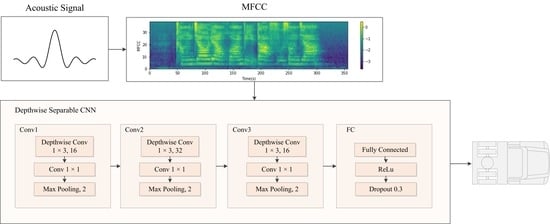
The CNN architecture is comprised of three convolution layers with two max-pooling layers between the three convolution layers and two fully connected layers for the output. The input channel numbers for the first, second and third convolution layers are 1, 16 and 32 respectively; the output channels are 16, 32 and 16, and the kernel sizes are 3, 3 and 3. For each layer, the stride and padding sizes are all set to 1. The kernel sizes for max pooling are 2. The framework structure of the CNN is shown in

Table 3. The CNN structure.

Layer	Parameters
Conv1d	1 × 16 × 3
Max Pooling	2
Conv1d	16 × 32 × 3
Max Pooling	2
Conv1d	32 × 16 × 3
Flatten	-
Fully Connected	144 × 16
Relu	-
Dropout	0.3
Fully Connected	16 × 2

.

A depthwise separable CNN architecture is trained for comparison with the same parameter settings as the original CNN structure. The convolution steps are replaced with depthwise separable convolution.

3. Results

3.1. Detection Accuracy

The frame-level accuracy and performance of the proposed method are evaluated on the test set of the vehicle recordings.

The training loss and validation loss of the DS CNN are shown in Figure 6. Figure 6A shows the training loss for each iteration, and Figure 6B shows the validation loss for each epoch. The decaying trends for the loss function of the training set and the validation set are consistent. The batch size is 128, and there are overall 100 epochs and 156,250 iterations. It can be seen that the loss function starts to converge at the 60th epoch, and therefore it is reasonable to choose the 100th epoch to stop training. Figure 7A shows the accuracy of the validation set for each epoch of the DS CNN. The confusion matrix of the DS CNN is illustrated in Figure 7B. The precision rate is 92.87%, the recall rate is 96.70%, and the false alarm rate is 7.42%.

The frame-level classification results of the proposed models are given in

Table 4. The overall detection accuracy of each model.

Framework	Classification Accuracy (%)
Two-stage Detection	93.65
DNN	89.88
CNN	93.02
DS CNN	92.58
DNN (Spec Augmentation)	92.14
CNN (Spec Augmentation)	95.11
DS CNN (Spec Augmentation)	94.64

. The accuracy of our baseline system, two-state detection is 93.65%. The classification accuracy results for the DNN, the CNN and the depthwise separable CNN models, are $89.88\%$, $93.02\%$ and $92.58\%$, respectively. The accuracy results with data augmentation for the DNN, the CNN and the depthwise separable CNN models, are $92.14\%$, $95.11\%$ and $94.64\%$, respectively. It can be seen that the classification accuracy is improved with augmentation.

To test the models’ ability to detect different types of vehicle, a test was conducted on different types of vehicles separately, and the result is shown in

Table 5. The ability to detect different types of vehicle of the models.

Method	Two-Stage	DNN	CNN	DS CNN	DNN	CNN	DS CNN
Remark	(9.9 dB)	without SpecAug			with SpecAug
SWV(91)	74.09	85.93	87.55	86.11	86.94	90.01	89.45
LWV(101)	96.45	90.41	93.88	93.63	93.01	96.06	95.58
TV(62)	96.81	91.01	94.48	94.28	93.49	96.36	95.93
Recall rate(254)	96.61	89.62	94.31	93.61	92.91	96.98	96.70
False alarm rate	9.31	9.86	8.27	8.45	8.63	6.76	7.42

. The numbers in the brackets of the first column are the numbers of vehicle recordings of different types. All the accuracy results are in frame-level. The traditional subspace-based target detection method has high accuracy towards the large wheeled vehicle and the tracked vehicle because the two types of vehicles make louder sounds when starting, leading to a higher SNR, and the threshold is optimized for these cases. However, the traditional method does not have a good performance for the small wheeled vehicle, as it makes a lower sound, especially when the sensors are placed far from the moving target, causing a low SNR. The DS CNN structure outperform the traditional method on both recall rate and false alarm rate.

3.2. Complexity Calculation

In the original CNN structure, there are three layers of CNN networks. According to Equations (5) and (6), the computation cost, C, for the first convolution layer is:

$$C=D_K^p\times M\times N\times D_F^p=3^1\times 1\times 16\times 1^1=48$$

(11)

The computation cost for the first depthwise separable convolution layer is:

$$C=D_K^p\times M\times D_F^p+M\times N\times D_F^p=3^1\times 1\times 1^1+1\times 16\times 1^1=19$$

(12)

According to Equation (7), the computation ratio, R, is:

$$R=1/N+1/D_k^p=1/16+1/3^1=19/48=39.58\%$$

(13)

The computation costs including the remaining two layers are shown in

Table 6. The computation cost of each convolution layer.

Convolution Layer	Original Cost	DS Cost	Reduction Rate(%)
1	48	19	60.42
2	1536	560	63.54
3	1536	608	60.42
All	3120	1187	61.96

. It can be seen that overall cost is reduced 61.96%in the convolution steps.

According to

Table 7. The number of parameters of each model.

Model	Number of Parameters
DNN	4922
CNN	5538
DS CNN	3654

, the overall parameter number is 5538 for the original CNN network, and the parameter number is 3654 after applying the depthwise separable CNN. The number of parameters reduced by 34.02% with only a small reduction of accuracy of 0.47%.

4. Discussion

The final model migrated to the chips of the sensors is the depthwise separable CNN. The model is lightweight and can be run efficiently on the chips of the sensors. For each frame, the average processing time is about 20 ms; thus, the real-time rate for each frame is $10\%$. The remaining computational resources can be utilized for other functions such as direction of arrival. The other reason for choosing a depthwise separable convolution network is to prolong the battery life. The intelligent sensor system has to be placed outdoors in the field over weeks. Therefore, the power consumption has to be limited. There is a trade-off between accuracy and model size, and finally the decrease in the accuracy is totally acceptable.

Figure 8 shows the signal and actual detection result of a sample. Figure 8A is the original time-domain signal of a large wheeled vehicle sample. Figure 8B shows some detection errors exist near the border region between the silence part and vehicle moving stage. Figure 8C shows the detection result after applying a smoothing function. Figure 8D represents the ground truth. The recorded moving time of the vehicle is from the 16th second to the 89th second. It can be seen that most classification errors occur at the border region between the silence part and the vehicle moving stage. This can be solved subsequently using a moving window to smooth. The detection algorithm is processed once every 200 milliseconds for each frame, and the detection result is transmitted every 1 s through the transmission module. Therefore, the following strategy is taken for smoothing: the final detection result follows the majority results of the five frames over a second.

Other classification errors occur when strong environment noise such as wind noise exists, and the distance between sensors and the vehicle is too long. In such cases, the signal-to-noise ratio becomes low, especially for a small wheeled vehicle, and the classification accuracy becomes affected. In the future, we intend to solve this problem by exploring signal processing methods including filtering and signal enhancement.

5. Conclusions

This paper proposes a CNN architecture with spectrogram augmentation for vehicle detection. A fully connected network and convolution neural networks are compared, and the CNN structure outperforms the other one. The depthwise separable CNN structure reduces the computational cost. Spectrogram augmentation also shows a huge improvement in the overall model performance. Experiments show that the DS CNN increases the recall rate of detection and reduces the false alarm rate simultaneously compared with the older two-stage method. The accuracy, recall rate and false alarm rate are 94.64%, 96.70% and 7.42%. Finally, the trained model is migrated to the chips of our intelligent sensor systems. The lightweight CNN model can be run efficiently on the these systems. Experiments show the structure has a robust and efficient performance on the sensors. In the future, we intend to discover some practical signal processing methods including filtering and a deep-learning-based signal denoising method to make the system more robust to wind noise and enhance the SNR.

References

1. Dawton, B.; Ishida, S.; Arakawa, Y. C-AVDI: Compressive measurement-based acoustic vehicle detection and identification. IEEE Access 2021, 9, 159457–159474. [Google Scholar] [CrossRef]
2. Dawton, B.; Ishida, S.; Hori, Y.; Uchino, M.; Arakawa, Y.; Tagashira, S.; Fukuda, A. Initial evaluation of vehicle type identification using roadside stereo microphones. In Proceedings of the IEEE Sensors Applications Symposium (SAS), Kuala Lumpur, Malaysia, 9–11 March 2020; pp. 1–6. [Google Scholar]
3. Dawton, B.; Ishida, S.; Hori, Y.; Uchino, M.; Arakawa, Y. Proposal for a compressive measurement-based acoustic vehicle detection and identification system. In Proceedings of the IEEE 92nd Vehicular Technology Conference (VTC2020-Fall), Virtual, 18 November–16 December 2020; pp. 1–6. [Google Scholar]
4. Fang, J.; Meng, H.; Zhang, H.; Wang, X. A low-cost vehicle detection and classification system based on unmodulated continuous-wave radar. In Proceedings of the IEEE Intelligent Transportation Systems Conference, Bellevue, DC, USA, 30 September–3 October 2007; pp. 715–720. [Google Scholar]
5. Wang, X. Vehicle image detection method using deep learning in UAV video. Comput. Intell. Neurosci. 2022, 2022. [Google Scholar] [CrossRef]
6. Kumari, S.; Agrawal, D. A Review on Video Based Vehicle Detection and Tracking using Image Processing. Int. J. Res. Publ. Rev. 2022, 2582, 7421. [Google Scholar]
7. Allegro, G.; Fascista, A.; Coluccia, A. Acoustic Dual-function communication and echo-location in inaudible band. Sensors 2022, 22, 1284. [Google Scholar] [CrossRef] [PubMed]
8. Gencoglu, O.; Virtanen, T.; Huttunen, H. Recognition of acoustic events using deep neural networks. In Proceedings of the 22nd European signal processing conference (EUSIPCO), Lisbon, Portugal, 1–5 September 2014; pp. 506–510. [Google Scholar]
9. Bae, S.H.; Choi, I.K.; Kim, N.S. Acoustic scene classification using parallel combination of LSTM and CNN. In Proceedings of the Detection and Classification of Acoustic Scenes and Events 2016, Budapest, Hungary, 3 September 2016; pp. 11–15. [Google Scholar]
10. Fu, R.; He, J.; Liu, G.; Li, W.; Mao, J.; He, M.; Lin, Y. Fast seismic landslide detection based on improved mask R-CNN. Remote Sens. 2022, 14, 3928. [Google Scholar] [CrossRef]
11. Li, H.; Lu, J.; Tian, G.; Yang, H.; Zhao, J.; Li, N. Crop classification based on GDSSM-CNN using multi-temporal RADARSAT-2 SAR with limited labeled data. Remote Sens. 2022, 14, 3889. [Google Scholar] [CrossRef]
12. Li, S.; Fu, X.; Dong, J. Improved ship detection algorithm based on YOLOX for SAR outline enhancement image. Remote Sens. 2022, 14, 4070. [Google Scholar] [CrossRef]
13. Adapa, S. Urban sound tagging using convolutional neural networks. arXiv 2019, arXiv:1909.12699. [Google Scholar]
14. Sharma, G.; Umapathy, K.; Krishnan, S. Trends in audio signal feature extraction methods. Appl. Acoust. 2020, 158, 107020. [Google Scholar] [CrossRef]
15. Vikaskumar, G.; Waldekar, S.; Paul, D.; Saha, G. Acoustic scene classification using block based MFCC features. In Proceedings of the IEEE AASP Challenge on Detection and Classification of Acoustic Scenes and Events (DCASE), Budapest, Hungary, 3 September 2016. [Google Scholar]
16. Ma, Y.; Liu, M.; Zhang, Y.; Zhang, B.; Xu, K.; Zou, B.; Huang, Z. Imbalanced underwater acoustic target recognition with trigonometric loss and attention mechanism convolutional network. Remote Sens. 2022, 14, 4103. [Google Scholar] [CrossRef]
17. Chaudhary, M.; Prakash, V.; Kumari, N. Identification vehicle movement detection in forest area using MFCC and KNN. In Proceedings of the 2018 International Conference on System Modeling & Advancement in Research Trends (SMART), Moradabad, India, 23–24 November 2018; pp. 158–164. [Google Scholar]
18. Pons, J.; Serra, X. Randomly weighted cnns for (music) audio classification. In Proceedings of the ICASSP 2019–2019 IEEE International Conference on Acoustics, Speech and Signal Processing (ICASSP), Brighton, UK, 12–17 May 2019; pp. 336–340. [Google Scholar]
19. Stowell, D.; Plumbley, M.D. Automatic large-scale classification of bird sounds is strongly improved by unsupervised feature learning. PeerJ 2014, 2, e488. [Google Scholar] [CrossRef] [PubMed]
20. Kinnunen, T.; Chernenko, E.; Tuononen, M.; Fränti, P.; Li, H. Voice activity detection using MFCC features and support vector machine. In Proceedings of the Int. Conf. on Speech and Computer (SPECOM07), Moscow, Russia, 4–10 August 2007; Volume 2, pp. 556–561. [Google Scholar]
21. Thomas, S.; Ganapathy, S.; Saon, G.; Soltau, H. Analyzing convolutional neural networks for speech activity detection in mismatched acoustic conditions. In Proceedings of the 2014 IEEE International Conference on Acoustics, Speech and Signal Processing (ICASSP), Florence, Italy, 4–9 May 2014; pp. 2519–2523. [Google Scholar]
22. Tokozume, Y.; Ushiku, Y.; Harada, T. Learning from between-class examples for deep sound recognition. arXiv 2017, arXiv:1711.10282. [Google Scholar]
23. Salamon, J.; Bello, J.P. Deep convolutional neural networks and data augmentation for environmental sound classification. IEEE Signal Process. Lett. 2017, 24, 279–283. [Google Scholar] [CrossRef]
24. Ko, T.; Peddinti, V.; Povey, D.; Khudanpur, S. Audio augmentation for speech recognition. In Proceedings of the Sixteenth Annual Conference of the International Speech Communication Association, Dresden, Germany, 6–10 September b2015. [Google Scholar]
25. Piczak, K.J. Environmental sound classification with convolutional neural networks. In Proceedings of the IEEE 25th international workshop on machine learning for signal processing (MLSP), Boston, MA, USA, 17–20 September 2015; pp. 1–6. [Google Scholar]
26. Park, D.S.; Chan, W.; Zhang, Y.; Chiu, C.C.; Zoph, B.; Cubuk, E.D.; Le, Q.V. Specaugment: A simple data augmentation method for automatic speech recognition. arXiv 2019, arXiv:1904.08779. [Google Scholar]
27. Krizhevsky, A.; Sutskever, I.; Hinton, G.E. Imagenet classification with deep convolutional neural networks. Adv. Neural Inf. Process. Syst. 2012, 25. [Google Scholar] [CrossRef]
28. Denil, M.; Shakibi, B.; Dinh, L.; Ranzato, M.; De Freitas, N. Predicting parameters in deep learning. Adv. Neural Inf. Process. Syst. 2013, 26. [Google Scholar]
29. Howard, A.G.; Zhu, M.; Chen, B.; Kalenichenko, D.; Wang, W.; Weyand, T.; Andreetto, M.; Adam, H. Mobilenets: Efficient convolutional neural networks for mobile vision applications. arXiv 2017, arXiv:1704.04861. [Google Scholar]
30. Huang, J.; Zhang, X.; Guo, F.; Zhou, Q.; Liu, H.; Li, B. Design of an acoustic target classification system based on small-aperture microphone array. IEEE Trans. Instrum. Meas. 2014, 64, 2035–2043. [Google Scholar] [CrossRef]
31. Zhang, X.; Huang, J.; Song, E.; Liu, H.; Li, B.; Yuan, X. Design of small MEMS microphone array systems for direction finding of outdoors moving vehicles. Sensors 2014, 14, 4384–4398. [Google Scholar] [CrossRef]
32. Guo, F.; Huang, J.; Zhang, X.; Cheng, Y.; Liu, H.; Li, B. A two-stage detection method for moving targets in the wild based on microphone array. IEEE Sensors J. 2015, 15, 5795–5803. [Google Scholar] [CrossRef]
33. Zhang, X.L.; Wu, J. Deep belief networks based voice activity detection. IEEE Trans. Audio, Speech Lang. Process. 2012, 21, 697–710. [Google Scholar] [CrossRef]
34. Picone, J.W. Signal modeling techniques in speech recognition. Proc. IEEE 1993, 81, 1215–1247. [Google Scholar] [CrossRef]
35. Bahmei, B.; Birmingham, E.; Arzanpour, S. CNN-RNN and data augmentation using deep convolutional generative adversarial network for environmental sound classification. IEEE Signal Process. Lett. 2022, 29, 682–686. [Google Scholar] [CrossRef]
36. Guo, J.; Li, Y.; Lin, W.; Chen, Y.; Li, J. Network decoupling: From regular to depthwise separable convolutions. arXiv 2018, arXiv:1808.05517. [Google Scholar]
37. Zhao, L.; Krishnaiah, P.R.; Bai, Z. On detection of the number of signals in presence of white noise. J. Multivar. Anal. 1986, 20, 1–25. [Google Scholar] [CrossRef] [Green Version]
38. Strand, O.M.; Egeberg, A. Cepstral mean and variance normalization in the model domain. In Proceedings of the COST278 and ISCA Tutorial and Research Workshop (ITRW) on Robustness Issues in Conversational Interaction, Norwich, UK, 30–31 August 2004. [Google Scholar]
39. Bottou, L. Large-scale machine learning with stochastic gradient descent. In Proceedings of the COMPSTAT’2010, Paris, France, 22–27 August 2010; pp. 177–186. [Google Scholar]
40. Srivastava, N.; Hinton, G.; Krizhevsky, A.; Sutskever, I.; Salakhutdinov, R. Dropout: A simple way to prevent neural networks from overfitting. J. Mach. Learn. Res. 2014, 15, 1929–1958. [Google Scholar]
Figure 1. The diagram of the system hardware architecture.
Remotesensing 14 04848 g001
Figure 2. The system hardware circuits layout.
Remotesensing 14 04848 g002
Figure 3. The recording scene.
Remotesensing 14 04848 g003
Figure 4. The diagram of MFCC extraction.
Remotesensing 14 04848 g004
Figure 5. The original log-mel spectrogram of a vehicle recording and the masked log-mel spectrogram.
Remotesensing 14 04848 g005
Figure 6. (A) The training loss vs. iteration; (B) the validation loss vs. epoch.
Remotesensing 14 04848 g006
Figure 7. (A) The accuracy of the validation data vs. epoch; (B) the confusion matrix of the DS CNN.
Remotesensing 14 04848 g007
Figure 8. Example of the original signal of a recording and its detection results: (A) the original signal of a recording; (B) the detection result of the recording; (C) the smoothed result; (D) the detection ground truth.
Remotesensing 14 04848 g008