Article

RGB-ICP Method to Calculate Ground Three-Dimensional Deformation Based on Point Cloud from Airborne LiDAR

1
School of Geosciences and Info-Physics, Central South University, Changsha 410083, China
2
Laboratory of Geohazards Perception, Cognition and Predication, Central South University, Changsha 410083, China
*
Author to whom correspondence should be addressed.
Remote Sens. 2022, 14(19), 4851; https://doi.org/10.3390/rs14194851
Submission received: 23 July 2022 / Revised: 24 September 2022 / Accepted: 26 September 2022 / Published: 28 September 2022

Abstract

:
With the rapid development of LiDAR technology in recent years, high-resolution LiDAR data possess a great capability to describe fine surface morphology in detail; thus, differencing multi-temporal datasets becomes a powerful tool to explain the surface deformation process. Compared with other differencing methods, ICP algorithms can directly estimate 3D displacements and rotations; thus, surface deformation parameters can be obtained by aligning window point clouds. However, the traditional ICP algorithm usually requires a good initial pose of the point cloud and relies on calculating the spatial distance to match the corresponding points, which can easily lead the algorithm to the local optimum. To address the above problems, we introduced the color information of the point cloud and proposed an improved ICP method that fuses RGB (RGB-ICP) to reduce the probability of matching errors by filtering color-associated point pairs, thus improving the alignment accuracy. Through simulated experiments, the ability of the two algorithms to estimate 3D deformation was compared, and the RGB-ICP algorithm could significantly reduce the deformation deviation (30–95%) in the three-dimensional direction. In addition, the RGB-ICP algorithm was applicable to different terrain structures, especially for smooth terrain, where the improvement was the most effective in the horizontal direction. Finally, it is worth believing that the RGB-ICP algorithm can play a unique role in surface change detection and provide a reliable basis for explaining the surface motion process.

1. Introduction

Ground deformation is a common surface process, including common phenomena such as surface subsidence, ground cracking, and mountain collapse. Surface deformation affects regional economic development and the life safety of residents, and monitoring surface deformation is a serious economic and environmental challenge [1]. Currently, contactless observation of surface deformation processes can be achieved using remote sensing techniques, including Close-Range Photogrammetry, Synthetic Aperture Radar (SAR), Global Positioning System (GPS), and Light Detection and Ranging (LiDAR) [2]. LiDAR technology is mainly used to acquire accurate 3D structural information by emitting lasers to densely sample the target surface [3], thus assisting in the integrated observation of space–air–ground [4,5,6]. LiDAR systems can be classified according to different platforms, including satellite-based, airborne, mobile ground, and maritime [3]. The unique advantages of LiDAR over other remote sensing technologies are reflected in the automatic filtering of surface vegetation and the rapid generation of fine-scale terrain products on a large sub-meter scale [7]. Airborne laser scanning (ALS) is now widely recognized as a fundamental tool for conducting scientific investigations of the Earth’s surface [8], offering new opportunities for understanding the Earth’s surface processes. In recent years, high-resolution ALS has been successfully applied to glacier movement [9,10], volcanic eruptions [11,12], floods [13,14], shoreline measurements [15], landslides [16,17,18], earthquakes [19,20,21,22,23,24], and other fields [25,26]. These cases also demonstrate the great potential of high-resolution LiDAR topographic data to describe and detect surface morphology in detail.
High-resolution ALS data contain more fine surface morphological information [7], and collecting repeated ALS data can accurately analyze surface deformation processes and reveal the underlying mechanisms of changes. A common method for surface change monitoring using multi-temporal ALS is DEM differencing (DoD) [27], which captures surface change processes by subtracting a two-phase raster. This method is simple in principle and suitable for flat areas or vertical surface deformation, but it ignores horizontal displacements [19,28], and the fidelity of the acquired vertical deformation is sometimes unreliable. In addition, particle image velocimetry (PIV) [29] and the co-registration of optically sensed images and correlation (COSI-Corr) [30] are also commonly used. LiDAR data can be converted to images, and PIV mainly intercorrelates grating images for successive observation periods, thus estimating the in-plane velocity field. Meanwhile, COSI-Corr is another image-based method that focuses on the accurate alignment and sub-pixel correlation of multi-temporal laser intensity images. Both methods can obtain highly accurate horizontal displacement estimates, for example, horizontal estimates in the 2014 South Napa, CA, earthquake are generally consistent with field measurements [22,31]. Since it provides a non-rigid transformation, it can accurately interpret the Earth’s surface phenomena. However, these two methods essentially measure 2D changes [32], and in reality, surface deformation occurs in arbitrary 3D directions [33].
The iterative closest point (ICP) [34,35] is a classical point cloud alignment method that allows 3D displacements and rotations to be calculated by aligning point clouds within the pre-event and post-event windows and ultimately directly estimating surface 3D deformation. Nissen et al [36] first applied this method to calculate simulated displacements on the San Andreas Fault in California and demonstrated its potential to calculate 3D deformation. Subsequently, the use of the ICP method has since had many successful applications for estimating 3D surface deformation [21,22,37,38,39]. However, the ICP algorithm requires a good overlap of the original point cloud to achieve good alignment during the iterative process, and while surface deformation is computed as the best rigid transformation, the assumption does not accurately model many natural phenomena [32]. It is worth noting that the traditional ICP approach must balance the choice of cell sizes to include larger scales for more terrain while not violating the rigid body assumption [36]. The ICP can provide spurious deformation estimates when local areas lack sufficient terrain undulation characteristics [38]; for example, a study [37] noted that during the El Mayor-Cucapah earthquake, the displacements calculated using the ICP method were spurious on the Laguna Salada plain.
In summary, the traditional ICP algorithm applied to ground deformation monitoring still has several limitations. It is interesting work to improve ICP algorithms in order to provide more accurate 3D deformation estimates. With the development of depth sensing techniques such as structured light, it is feasible to capture both color and distance information [40], and RGB-D depth images from color cameras can be associated with 3D point clouds to generate color point clouds with distance and texture information. The traditional ICP algorithm aligns two major datasets by computing 3D spatial distances. However, geometry-based alignment is sometimes not always accurate [41], and the addition of color information can assist in determining the nearest points for fast convergence [42] and improve the ICP alignment accuracy. Based on the above analysis, the ICP method, by fusing color information, has great potential to improve the accuracy of surface deformation monitoring. Thus, we tried to fuse RGB information with the window ICP method and to analyze the ability of this method to estimate 3D deformation by adding simulated displacements to the color point cloud and obtained the results of the comparison with the standard window ICP method. Section II of this paper introduces the principles of the algorithms of the standard ICP and RGB-ICP as well as the experimental data; Section III gives the comparison results of the RGB-ICP and standard ICP for 3D differencing; Section IV mainly discusses the shortcomings and potentials of the RGB-ICP algorithm; Section V gives the conclusions from this study.

2. Methodology

2.1. Methods

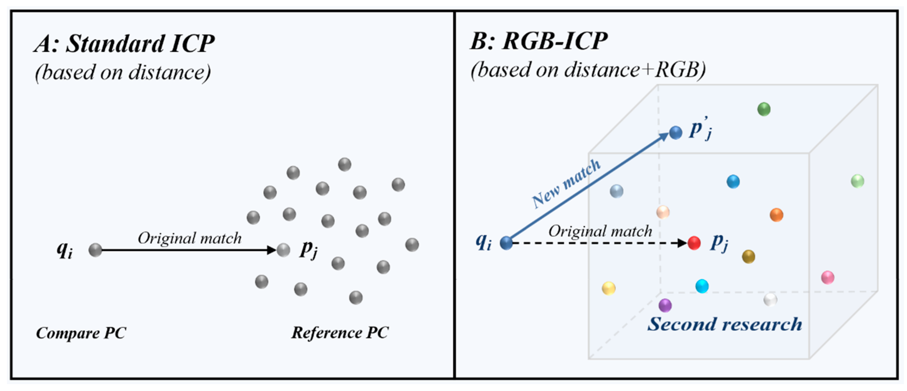
2.1.1. Standard ICP Method

The traditional ICP algorithm is an alignment method based on 3D geometric features. Given a group of moved point sets Q = { q i Q , i = 1 , , N q } and a group of fixed point sets P = { p j P , j = 1 , , N p } , the alignment of two groups of point sets is achieved by continuously transforming the moving points through successive iterations, which mainly consists of the below steps.
Let us assume the initial transformation M 0 = [ R 0 , T 0 ] , where R 0 = I , T 0 = 0 (I is the unit matrix):
1.
Match: Usingor transformation matrix M0 or transformation matrix Mk1 after the last iteration, the set of moving points, Q, is transformed, and the nearest point pi corresponding to each point qi is found by calculating the spatial three-dimensional Euclidean distance, where the distance between point qi and point sets P is defined as follows:
d ( q i , P ) = min j = 1 , , N p d ( q i , p j )
Here, the nearest point set is set to Y = { p i P , i = 1 , 2 , , N q } , at which time there is a single mapping relationship between the two groups of point sets. Meanwhile, finding the spatial nearest points would take a lot of time, and the query efficiency can be improved by building a 3-dimensional KD tree [43,44].
2.
Transform: Moving the set of points, Q, under a given spatial transformation including rotation R and translation T minimizes the distance error metric between matched pairs of points, at which point the solved M k = [ R k , T k ] is the optimal transformation. The literature [34,35] gives two different ways of error metrics.
The point-to-point minimization is:
M k = argmin M k 1 i = 1 N q M k 1 · q i p i 2
The point-to-plane minimization is:
M k = argmin M k 1 i = 1 N q ( M k 1 · q i p i ) · n i 2
Here, ni is the corresponding normal projection vector of pi. Regarding how to solve the optimal spatial transformation, M, common methods include the singular value decomposition method (SVD) [45], the quaternion method [46], and the dual quaternion method [47].
3.
Iterative calculation and threshold judgment: After applying the optimal transformation to the set of moving points, Q, the above steps are repeated to complete the next iterative transformation. The ICP algorithm can define the absolute increment of rotation Rd and translation Td during successive iterations as the basis for judgment:
{ R d = | R k R k 1 | T d = | T k T k 1 |
Generally, the ICP algorithm terminates when Rd and Td are smaller than the corresponding thresholds or when the number of iterations, k, reaches the upper limit.
The ICP algorithm requires good initial transformation parameters [48]; otherwise, the iterative solution tends to fall into a local optimum. Currently, many variants were derived based on the standard ICP algorithm, mainly based on the six phases of the algorithm [49]: selection, matching, weighting, the rejection of erroneous point pairs, the assignment of error metric, and metric minimization, for example, point matching using information such as intensity [50] and color [51], the adaptive rejection of matched point pairs [52,53], the computation of transformations using simulated annealing algorithms [54], etc. However, the comparison of variants focuses on the convergence speed of the algorithm [55], and less attention is paid to the stability and accuracy of the rigid transformation [56].

2.1.2. Improved RGB-ICP Method

The idea of adding color information to the ICP algorithm to facilitate the accurate alignment of texture point clouds is not fresh, and current research [57] can use color information in both the “matching” and “error metric minimization” processes. For example, Johnson and Kang [41] proposed a 6D l2 color distance, which adds color differences to the Euclidean distance metric, but the algorithm does not eliminate the dimensional differences between spatial distance and pixel intensity. In addition to this, a 4D ICP structure [58,59] was also proposed to add hue values to the spatial 3D structure to improve the point pair matching accuracy; meanwhile, how to assign weight values to the distance part and hue part, as well as normalize the difference between them, is the key task of the weighted hue ICP algorithm [58]. Of course, there is also the direct use of color information to optimize point pair matching [60], mainly by re-searching a number of neighboring points for filtering. Most studies add color information to the point pair matching process, while error metric minimization using color tends to fail to converge properly [57] and is not applicable to the case of complex color mutations.
In summary, this study synthesizes the basic ideas of the color-assisted ICP algorithm and proposes a traditional ICP method that incorporates color information. Compared with the traditional ICP algorithm, this method optimizes and filters matched point pairs by adding RGB information, and the specific principles are as follows:
  • For a set of associated point pairs, the nearest point pj is used as the core to expand the range to search the neighboring points, and all neighboring points under this search domain, Ω, are defined as candidate points. The search methods include: the KNN neighboring algorithm, sphere division, and cubic dissection;
  • The RGB distance between moving point qi and candidate points is calculated (Equation (5)), and the most similar color point p j is selected:
    d ( q i , p j ) = ( q i R p j R ) 2 + ( q i G p j G ) 2 + ( q i B p j B ) 2
  • After color filtering, the acquired new matching point pairs continue to participate in subsequent calculations.
For the secondary filtering of matched point pairs, the purpose is to ensure that points with similar spatial distance and color are aligned to reduce the probability of false matches. Figure 1 shows the process of screening point pairs before and after the improvement in the ICP algorithm, and here, the modified algorithm illustrates the basic principle of secondary screening with a cubic search domain of specified step size.
The traditional ICP method mainly provides a rigid estimation of 3D pose by aligning the point clouds within the pre-event and post-event windows. For the pre and post point clouds, the point set needs to be gridded first, and the core of mesh is used as a reference to establish a set of points to be aligned. All points within the two-phase windows are searched separately with these points to be aligned as the core; the ICP alignment is performed after defocusing the point sets, and the estimated best rigid transformation is regarded as the 3D deformation component. The innovation of the RGB-ICP algorithm lies in the second filtering of point pairs; the first matching is based on spatial distance calculation, while the second filtering determines the color similarity between all points in the domain and the target point by expanding the neighborhood. The size of the search domain can be defined by itself; when the color distance (Equation (5)) is minimum then the corresponding point is the new matching point. The second filtering greatly reduces the probability of false matching, significantly decreases the false pose estimation caused by arbitrary alignment, and improves the accuracy of the window ICP algorithm in estimating the 3D pose. The specific flow can be seen in Figure 2.

2.2. Data

RGB images from a digital aerial camera can be correlated with three-dimensional point clouds to generate color point clouds with both spatial and textural information to support a fine-grained description of surface morphology. The experimental data were downloaded from the open access OpenTopography platform in LAS format, where all four ALS point clouds have color information to test the performance of the algorithm. In order to investigate the applicability of the RGB-ICP algorithm to different terrain structures, smooth terrain and rough terrain were selected here for comparison. To easily differentiate the two terrains, the point cloud was resampled as a 5 m resolution elevation grid, and its slope components in the east–west (E-W) and north–south (N-S) directions were separately calculated and finally summarized to obtain the overall mean value. Here, 5° was used as the final classification threshold based on the results of several experiments and visual interpretation. Consequently, smooth terrain was defined as the average slope less than or equal to 5°, such as plains; rough terrain was defined as the average slope more than 5°, such as hills or mountains. A total of 4 groups of sample data were downloaded for this experiment, and each group included 2 different terrain cases. The width of the point cloud ranged from 1.5 to 2.5 km, and other details can be found in Table 1.

3. Results

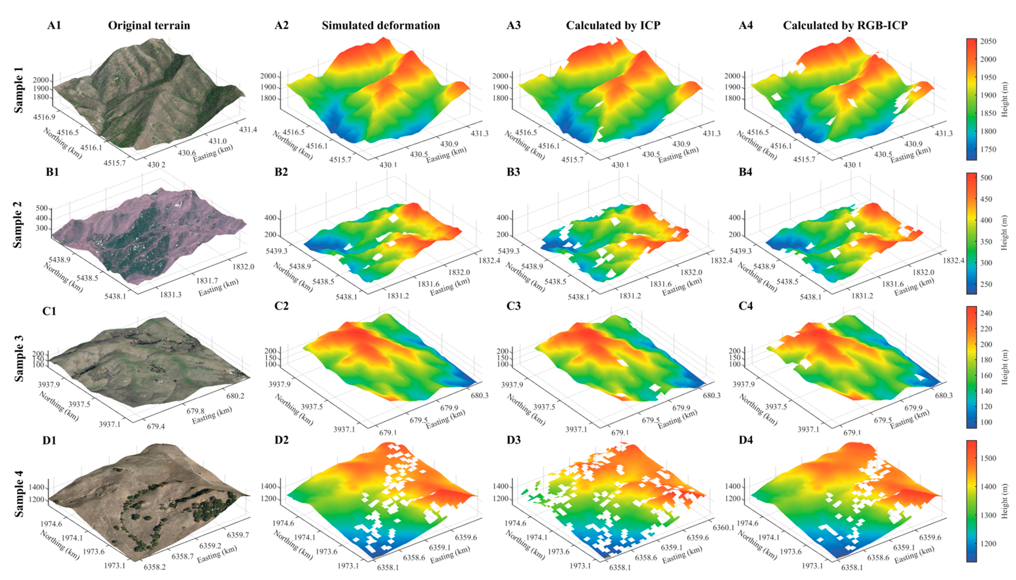
3.1. Simulated Deformation

The texture of the point cloud for actual surface deformation events is still difficult to obtain, so in order to investigate the improvement in this algorithm, the point cloud data were here synthesized to simulate 3D displacements, which meant that one deformation surface tilted in the E-W, N-S and vertical directions was defined. The deformation gradually increased along the diagonal to both sides with values ranging from 0 to 5 m. It was also highly adaptive for the global range of the point cloud to facilitate a comparative analysis of the results. The distribution of this synthetic displacement is given in Figure 3, where displacement is situated in the focus of each window, with black arrows indicating horizontal displacement and colored circles indicating vertical displacement. The window size was closely related to the point cloud density as well as the deformation and other factors; hence, a too large or too small window would have had an impact on the alignment results. Considering that the point cloud density used in the experiment lay in the range of 3–5 pts∙m−2, here, we chose a 40 × 40 m window, took the K-nearest neighbor search as an example, and used the point-to-plane minimization metric for the experiment. Meanwhile, to avoid having the ICP algorithm fall into the local optimum due to the insufficient points in a given window, we set the number of point cloud below 200 not to participate in the registration. Finally, we tested all the datasets using the above two algorithms separately.

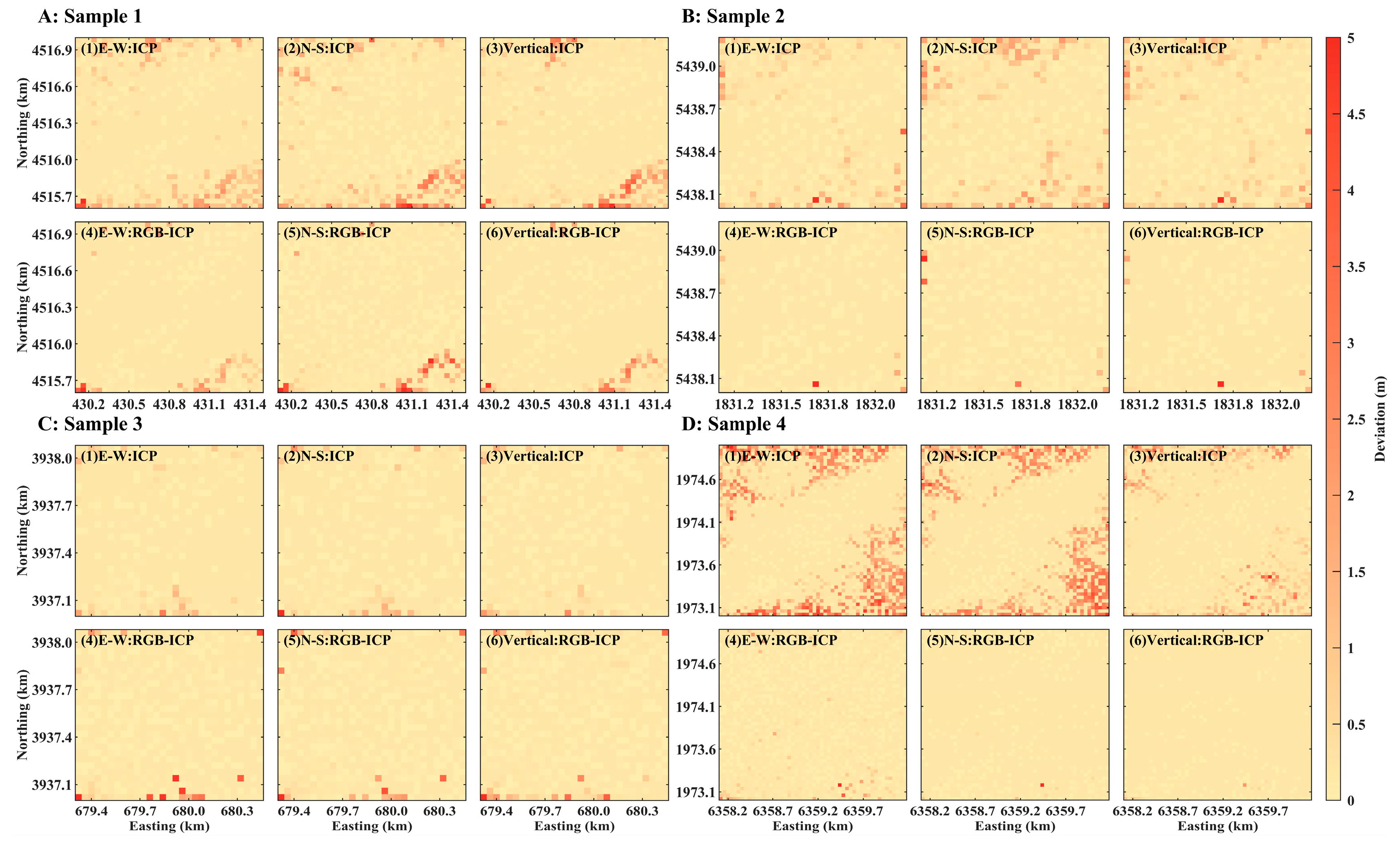
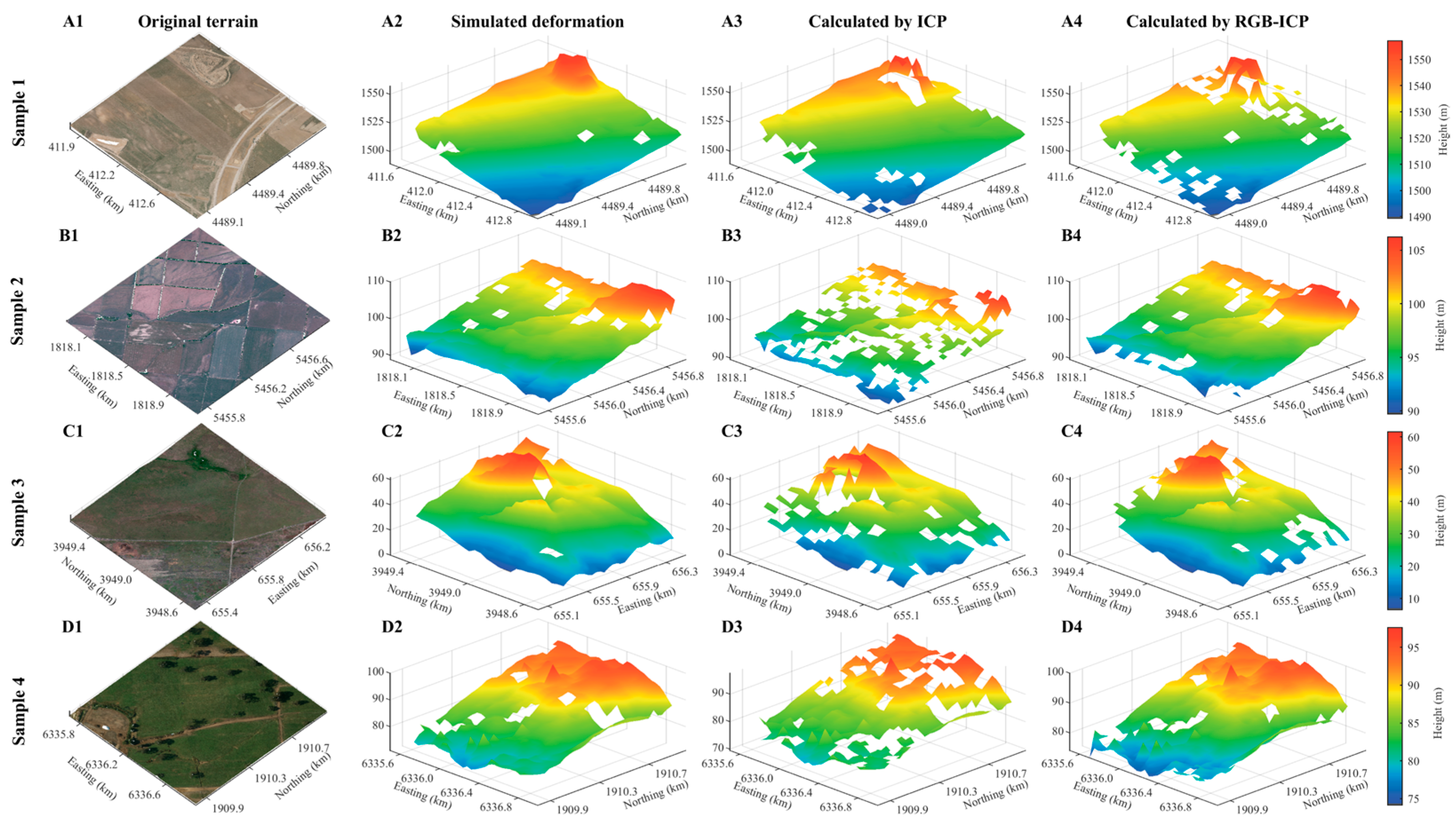
3.2. Experimental Results

3.2.1. Rough Terrain

After testing, we obtained the results of the two algorithms for estimating the 3D pose separately. First, the deformation values were superimposed on the original terrain to facilitate the overall comparison of the algorithm results. Taking rough terrain as an example, Figure 4 shows the overall calculation results of both algorithms. Since the larger simulated deformations were clustered on the northern and southern sides, the alignment effect of the two algorithms could be judged by observing whether the distribution of the terrain on both sides was consistent with the simulated terrain. Ignoring some of the missing meshes, the overall deformation results calculated using the two algorithms did not differ significantly from the simulated deformation, and the results of the four sets of samples fit the simulated terrain, which indicated that the difference in the alignment effects between the two algorithms was small. The rough terrain had more undulating structures, and the ICP algorithm could identify the corresponding points more accurately, so the traditional ICP algorithm had a relatively good alignment for undulating point clouds. Then, in order to quantify the error range, the deformation deviation results for rough terrain are given in Figure 5, where the x-axis and y-axis in each subplot represent the E-W and N-S directions, respectively, and the z-axis represents the deformation deviation range, which means the absolute difference between the simulated and calculated values. According to the comparison results of deformation deviation, it could be seen that the deformation deviations in all three directions after RGB optimization were reduced to different degrees. Among them, in sample 1, the number of error anomalies in the three directions was partially reduced, and the deformation error was decreased to a certain extent, but some of outliers on the lower right side were still not removed. In sample 2, the number of error anomalies in the three directions was significantly reduced, and the overall improvement in the deformation error was more outstanding. In sample 3, the contrast of deformation errors in the three directions was less obvious, and there were few outliers after RGB optimization, which needed to be judged according to the subsequent quantification results. In sample 4, the range of error anomalies in the three directions was significantly reduced, and the overall improvement in the deformation error was obvious, especially in the E-W and N-S directions. In summary, the error improvement effect of sample 4 was the best, and the other datasets also had some degree of improvement.

3.2.2. Smooth Terrain

The deformation deviation results for rough terrain reflected the robustness of the RGB-ICP algorithm; however, the improvement was not significant. To investigate the improvement potential of the RGB-ICP algorithm, the smooth terrain of each of the four datasets was also tested here (Figure 6 and Figure 7). By neglecting some of the missing meshes, the deformation results calculated using the RGB-ICP algorithm basically fit the simulated deformation better than the traditional ICP algorithm by observing the topographic distribution of the north and south sides, especially in sample 1 and sample 3, which indicated a better alignment of the RGB-ICP algorithm. Compared with rough terrain, smooth terrain lacked the terrain structure characteristics, and the spurious estimation caused by arbitrary spatial alignment affected the alignment results, especially in the E-W and N-S directions, while the window center of mass was easily vertically aligned, as it is usually better than the other directions. As can be seen from Figure 7, overall, the alignment characteristics of the ICP for smooth terrain were: the deformation deviation in the horizontal direction was large, and the alignment effect was poor, while the alignment effect in the vertical direction was good; then, the deformation deviation in the E-W and N-S directions was significantly reduced after RGB optimization, and the deviation in the vertical direction was also improved to some extent. In sample 1, the range of the error anomalies in the E-W and N-S directions was significantly decreased, and the deformation error was more obviously reduced, but there were still some outliers that could not be removed. In sample 2, the number of error anomalies in the E-W and N-S directions significantly dropped, and the improvement in the deformation error was more prominent, with a small number of anomalies on the top and bottom edges. In sample 3, the deformation errors in the E-W and N-S directions were significantly reduced, and very few anomalies still appeared at the edges. In sample 4, the number of error anomalies in the E-W and N-S directions significantly decreased and was basically close to 0. The improvement effect of deformation error was outstanding. In addition, since the comparison effect of the vertical error was not obvious in the two-dimensional display, a comprehensive analysis was carried out in the subsequent quantification of the deviation results, including the comparison results of the alignment accuracy among the sample data.

3.3. Overall Evaluation

In order to make a visual comparison of the improvement effect of the two algorithms, the mean absolute error (MAE) was here used as an evaluation index. The MAE is commonly used to measure the deviation between the calculated value and the simulated value and here was used to compare the accuracy of the two algorithms. The calculated results are shown in Table 2. Firstly, the improvement effect of the algorithm was here compared for each group of sample data for different types of terrain. For rough terrain, in group 1, the average deviation of deformation in the three directions was reduced from 0.49 m, 0.30 m, and 0.24 m to 0.18 m, 0.13 m, and 0.12 m; in group 2, the average deviation of deformation was reduced from 0.28 m, 0.38 m, and 0.21 m to 0.1 m, 0.09 m, and 0.07 m; in group 3, the average deviation of deformation was reduced from 0.21 m, 0.20 m, and 0.06 m to 0.13 m, 0.12 m, and 0.04 m; in group 4, the average deviation of deformation was reduced from 0.84 m, 0.85 m, and 0.16 m to 0.03 m, 0.04 m, and 0.02 m. Here, the best error improvement was found in group 4, and the alignment accuracy of the other three groups of data was improved to different degrees. For smooth terrain, in group 1, the average deviation of deformation in the three directions was reduced from 1.79 m, 1.68 m, and 0.09 m to 0.75 m, 0.62 m, and 0.04 m, respectively; in group 2, the average deviation of deformation was reduced from 2.34 m, 2.36 m, and 0.05 m to 0.23 m, 0.24 m, and 0.03 m, respectively; in group 3, the average deviation of deformation was reduced from 1.32 m, 1.26 m, and 0.06 m to 0.27 m, 0.24 m, and 0.03 m, respectively; in group 4, the average deviation of deformation was reduced from 1.35 m, 1.35 m, and 0.05 m to 0.04 m, 0.05 m, and 0.02 m, respectively. It could be seen that the range of deformation error reduction varied for each data group, but group 4 had the best improvement, followed by group 2, group 3, and group 1.
Then, the improvement in the algorithm was discussed for the four groups of datasets as a whole. All four datasets showed a similar degree of accuracy improvement, with the most significant improvement in accuracy in group 4, followed by group 2. In group 1, the accuracy of the algorithm for both types of terrain improved by 45–65% after RGB optimization. In group 2, the accuracy of the algorithm for rough terrain improved by about 70% after RGB optimization, while the accuracy for smooth terrain improved by about 90% in the horizontal direction and by 39% in the vertical direction. In group 3, the accuracy of the algorithm for rough terrain improved by about 40% in the horizontal direction and by 39% in the vertical direction after RGB optimization; the accuracy for smooth terrain in the horizontal direction improved by about 80%, and the accuracy in the vertical direction improved by 52%. In group 4, the accuracy of the algorithm for both types of terrain improved by more than 90% after RGB optimization, except for the accuracy for smooth terrain in the vertical direction, which improved by 56%. Finally, according to the vertical comparison, the RGB-ICP algorithm had the most apparent improvement in the alignment effect in the horizontal direction for smooth terrain, and the accuracy improvement space for smooth terrain was larger than that for rough terrain, which was mainly reflected in group 3. In summary, after the experimental analysis, the RGB-ICP algorithm had higher alignment accuracy than the traditional ICP, as it could effectively improve the case of misalignment, thus increasing the accuracy of 3D pose estimation. In addition, the algorithm was suitable for different terrain structures, especially to alleviate the false displacement estimation due to the lack of structural features. It is worth noting that for low-density point clouds (such as group 4), the advantage of RGB filtering seemed to play a more significant role, and the improvement was relatively better.

3.4. Window Size Effect

To facilitate the comparison of the deformation results, this simulation experiment was based on fixed window size. Window size has a certain effect on the registration effect as the study scale. Based on the above considerations, a smooth sample was here selected as the test sample for the experiment to explore the registration effects of the two algorithms using different windows. The test results are given in Figure 8, which shows the trend of the MAE with the increase in the window in the three directions. It can be seen from the figure that the error of the original ICP algorithm in the three directions increased as the window increased; after color optimization, the trend of the RGB-ICP algorithm in the horizontal direction became flat, and the overall error was reduced to less than 1 m, while the error in the vertical direction tended to increase, but the overall error was still lower than that of the ICP algorithm. It was apparent that the performance of the RGB-ICP algorithm was robust to the effect of window size, and the improvement in the horizontal direction in particular was quite impressive. Of course, a single experiment cannot be generalized, and the mechanism of the effect of window size needs to be explored in depth with multiple data and levels.

4. Discussion

We proposed a window ICP method incorporating color information to improve registration accuracy by filtering point pairs with color. Based on the simulated displacement experiment, the RGB-ICP algorithm could significantly reduce the deformation error value and effectively improve the fitting effect. The disadvantage was that the simulation matrix set in this experiment was relatively single, which meant that the three-dimensional deformation distribution in the final result tended to be consistent, which shows that it is difficult to replace the complex, real deformation situation with a simulated deformation. Of course, we tried to change the matrix to explore whether the different deformation distributions affected the robustness of the RGB-ICP algorithm; the results showed that the RGB-ICP algorithm did not lose its unique advantage over the traditional ICP algorithm due to the deformation distribution, and its improvement effect was reliable and stable. It is worth noting that the effectiveness of the window ICP method depends not only on the algorithm itself, but also on the window size, point cloud density, and deformation [36,61]. After discussing the effect of window size on the algorithm, it is worthwhile to investigate the mechanism of factors such as point cloud density, deformation, or multi-factor interaction on the alignment effect of the RGB-ICP algorithm as future research work. In addition, in the deformation deviation results, even after RGB optimization, many sample data edges showed large errors (sample 1 and sample 3 for rough terrain; sample 2 and sample 3 for smooth terrain) due to the fact that edge windows that include larger deformations are more prone to mismatching and produce distortions. Without violating the assumption of rigidity, enlarging the window can support good registration by accommodating more deformation information, but at the same time, it reduces the accuracy of the study, so the suitable selection of window size [61] is important for proper pose estimation, and it is interesting to see whether color optimization can improve the limitation of narrow windows.
The algorithm requires additional time cost due to the inclusion of color filtering; thus, subsequent optimization needs to be performed more efficiently [62,63]. At the same time, the application of the window ICP method incorporating color is less mature, and its computational robustness for complex texture cases of real events still needs to be verified [64,65]. Finally, this algorithm relies on the manual adjustment of parameters, such as the search domain range; thus, the development of automated algorithms [66,67,68] remains the focus of future work. With the increasing growth of remote sensing datasets, the cooperative observation of optical and LiDAR provides opportunities and challenges for detecting surface morphology; thus, point cloud alignment incorporating color information has a promising future for measuring surface deformation.

5. Conclusions

In order to solve the situation whereby the traditional ICP algorithm incorrectly estimates 3D deformation due to arbitrary spatial alignment, we introduced RGB information into the ICP alignment algorithm and performed the secondary screening of matched point pairs based on color, thus reducing false matches. We tried to apply this algorithm to estimate the 3D deformation of ground surface and proposed a window ICP method that incorporated color information. Through synthetic displacement experiments, the ability of the RGB-ICP algorithm and the conventional ICP algorithm to estimate the 3D deformation was compared, and it was found that the RGB-ICP algorithm could effectively reduce the 3D deformation deviation. Taking the MAE as a reference, the accuracy of the algorithm in the 3D direction could be significantly improved by 30%~95%, including 40%~95% in the horizontal direction and 30%~90% in the vertical direction. At the same time, the ability of the RGB-ICP algorithm to measure 3D displacement was robust for different terrain structures, which could especially alleviate the situation of false displacement estimation in the horizontal direction for smooth terrain. Finally, the direct estimation of the 3D pose using the ICP algorithm is of great importance for the detection of near-real-time changes in the ground surface, and ICP variants are able to exploit its unique advantages over traditional algorithms, presenting great potential for measuring surface deformation and providing an important basis for near-surface motion processes (earthquakes, landslides, etc.).

Author Contributions

Conceptualization, W.W.; methodology, W.W.; software, M.S.; validation, M.S., W.W. and Y.P.; formal analysis, M.S. and W.W.; investigation, Y.P.; resources, M.S.; data curation, M.S.; writing—original draft preparation, M.S. and Y.P.; writing—review and editing, M.S. and Y.P.; visualization, Y.P.; supervision, W.W. and M.S.; project administration, W.W.; funding acquisition, W.W. All authors have read and agreed to the published version of the manuscript.

Funding

This study was supported by the National Key Research and Development Program of China (2018YFB0504500), the National Natural Science Foundation of China (41901295), Basic Science-Center Project of National Natural Science Foundation of China (72088101), the Natural Science Foundation of Hunan Province, China (2020JJ5708), and the Key Program of the National Natural Science Foundation of China (41930108).

Data Availability Statement

All datasets of this experiment can be found at OpenTopography (www.opentopography.org), including dataset 1 (https://doi.org/10.5069/G9TH8JNQ, accessed on 7 December 2021), dataset 2 (https://doi.org/10.5069/G9CV4FPT, accessed on 23 February 2022), dataset 3 (https://doi.org/10.5069/G9CN71V5, accessed on 7 June 2022), and dataset 4 (https://doi.org/10.5069/G9G73BM1, accessed on 13 June 2022). We express our sincere gratitude to the data providers and related agencies.

Acknowledgments

We sincerely thank the people who provided support and advice for this article.

Conflicts of Interest

The authors declare that no competing interests exist.

References

  1. Besoya, M.; Govil, H.; Bhaumik, P. A review on surface deformation evaluation using multitemporal SAR interferometry techniques. Spat. Inf. Res. 2021, 29, 267–280. [Google Scholar] [CrossRef]
  2. Zhang, F.; Pei, H.; Zhu, H.; Wang, L. Research review of large deformation monitoring of rock and soil. IOP Conf. Ser. Earth Environ. Sci. 2021, 861, 042030. [Google Scholar] [CrossRef]
  3. Dong, P.; Chen, Q. LiDAR Remote Sensing and Applications; CRC Press: Boca Raton, FL, USA, 2017. [Google Scholar]
  4. Liu, B.; Ma, X.; Ma, Y.; Li, H.; Jin, S.; Fan, R.; Gong, W. The relationship between atmospheric boundary layer and temperature inversion layer and their aerosol capture capabilities. Atmos. Res. 2022, 271, 106121. [Google Scholar] [CrossRef]
  5. Pei, Z.; Han, G.; Ma, X.; Shi, T.; Gong, W. A method for estimating the background column concentration of CO2 using the lagrangian approach. IEEE Trans. Geosci. Remote Sens. 2022, 60, 4108112. [Google Scholar] [CrossRef]
  6. Luo, B.; Yang, J.; Song, S.; Shi, S.; Gong, W.; Wang, A.; Du, L. Target classification of similar spatial characteristics in complex urban areas by using multispectral LiDAR. Remote Sens. 2022, 14, 238. [Google Scholar] [CrossRef]
  7. Tarolli, P. High-resolution topography for understanding Earth surface processes: Opportunities and challenges. Geomorphology 2014, 216, 295–312. [Google Scholar] [CrossRef]
  8. Glennie, C.L.; Carter, W.E.; Shrestha, R.L.; Dietrich, W.E. Geodetic imaging with airborne LiDAR: The Earth’s surface revealed. Rep. Prog. Phys. 2013, 76, 86801. [Google Scholar] [CrossRef]
  9. Geist, T.; Lutz, E.; Stötter, J. Airborne Laser Scanning Technology and Its Potential for Applications in Glaciology. Ph.D. Thesis, University of Innsbruck, Innsbruck, Austria, 2003. [Google Scholar]
  10. Joerg, P.C.; Morsdorf, F.; Zemp, M. Uncertainty assessment of multi-temporal airborne laser scanning data: A case study on an Alpine glacier. Remote Sens. Environ. 2012, 127, 118–129. [Google Scholar] [CrossRef]
  11. Albino, F.; Smets, B.; d’Oreye, N.; Kervyn, F. High-resolution TanDEM-X DEM: An accurate method to estimate lava flow volumes at Nyamulagira Volcano (DR Congo). J. Geophys. Res. Solid Earth 2015, 120, 4189–4207. [Google Scholar] [CrossRef]
  12. Behncke, B.; Fornaciai, A.; Neri, M.; Favalli, M.; Ganci, G.; Mazzarini, F. Lidar surveys reveal eruptive volumes and rates at Etna, 2007–2010. Geophys. Res. Lett. 2016, 43, 4270–4278. [Google Scholar] [CrossRef] [Green Version]
  13. Croke, J.; Todd, P.; Thompson, C.; Watson, F.; Denham, R.; Khanal, G. The use of multi temporal LiDAR to assess basin-scale erosion and deposition following the catastrophic January 2011 Lockyer flood, SE Queensland, Australia. Geomorphology 2013, 184, 111–126. [Google Scholar] [CrossRef]
  14. Bull, J.; Miller, H.; Gravley, D.; Costello, D.; Hikuroa, D.; Dix, J. Assessing debris flows using LiDAR differencing: 18 May 2005 Matata event, New Zealand. Geomorphology 2010, 124, 75–84. [Google Scholar] [CrossRef]
  15. Pye, K.; Blott, S.J. Assessment of beach and dune erosion and accretion using LiDAR: Impact of the stormy 2013–14 winter and longer term trends on the Sefton Coast, UK. Geomorphology 2016, 266, 146–167. [Google Scholar] [CrossRef]
  16. Burns, W.J.; Coe, J.A.; Kaya, B.S.; Ma, L. Analysis of elevation changes detected from multi-temporal LiDAR surveys in forested landslide terrain in western Oregon. Environ. Eng. Geosci. 2010, 16, 315–341. [Google Scholar] [CrossRef]
  17. DeLong, S.B.; Prentice, C.S.; Hilley, G.E.; Ebert, Y. Multitemporal ALSM change detection, sediment delivery, and process mapping at an active earthflow. Earth Surf. Processes Landf. 2012, 37, 262–272. [Google Scholar] [CrossRef]
  18. Lucieer, A.; Jong, S.M.d.; Turner, D. Mapping landslide displacements using Structure from Motion (SfM) and image correlation of multi-temporal UAV photography. Prog. Phys. Geogr. 2014, 38, 97–116. [Google Scholar] [CrossRef]
  19. Oskin, M.E.; Arrowsmith, J.R.; Corona, A.H.; Elliott, A.J.; Fletcher, J.M.; Fielding, E.J.; Gold, P.O.; Garcia, J.J.G.; Hudnut, K.W.; Liu-Zeng, J. Near-field deformation from the El Mayor–Cucapah earthquake revealed by differential LiDAR. Science 2012, 335, 702–705. [Google Scholar] [CrossRef]
  20. Nissen, E.; Maruyama, T.; Arrowsmith, J.R.; Elliott, J.R.; Krishnan, A.K.; Oskin, M.E.; Saripalli, S. Coseismic fault zone deformation revealed with differential lidar: Examples from Japanese Mw∼ 7 intraplate earthquakes. Earth Planet. Sci. Lett. 2014, 405, 244–256. [Google Scholar] [CrossRef]
  21. Clark, K.; Nissen, E.; Howarth, J.; Hamling, I.; Mountjoy, J.; Ries, W.; Jones, K.; Goldstien, S.; Cochran, U.; Villamor, P. Highly variable coastal deformation in the 2016 Mw7. 8 Kaikōura earthquake reflects rupture complexity along a transpressional plate boundary. Earth Planet. Sci. Lett. 2017, 474, 334–344. [Google Scholar] [CrossRef]
  22. Ekhtari, N.; Glennie, C. High-resolution mapping of near-field deformation with airborne Earth observation data, a comparison study. IEEE Trans. Geosci. Remote Sens. 2017, 56, 1598–1614. [Google Scholar] [CrossRef]
  23. Lajoie, L.J.; Nissen, E.; Johnson, K.L.; Arrowsmith, J.R.; Glennie, C.L.; Hinojosa-Corona, A.; Oskin, M.E. Extent of low-angle normal slip in the 2010 El Mayor-Cucapah (Mexico) earthquake from differential lidar. J. Geophys. Res. Solid Earth 2019, 124, 943–956. [Google Scholar] [CrossRef]
  24. Scott, C.; Bunds, M.; Shirzaei, M.; Toke, N. Creep along the Central San Andreas Fault from surface fractures, topographic differencing, and InSAR. J. Geophys. Res. Solid Earth 2020, 125, e2020JB019762. [Google Scholar] [CrossRef]
  25. Yin, T.; Cook, B.D.; Morton, D.C. Three-dimensional estimation of deciduous forest canopy structure and leaf area using multi-directional, leaf-on and leaf-off airborne lidar data. Agric. For. Meteorol. 2022, 314, 108781. [Google Scholar] [CrossRef]
  26. Xu, W.; Wang, W.; Wang, N.; Chen, B. A New Algorithm for Himawari-8 Aerosol Optical Depth Retrieval by Integrating Regional PM2.5 Concentrations. IEEE Trans. Geosci. Remote Sens. 2022, 60, 1–11. [Google Scholar]
  27. Wheaton, J.M. Uncertainity in Morphological Sediment Budgeting of Rivers. Original typescript. Ph.D. Thesis, University of Southampton, Southampton, UK, 2008. [Google Scholar]
  28. Duffy, B.; Quigley, M.; Barrell, D.J.; Van Dissen, R.; Stahl, T.; Leprince, S.; McInnes, C.; Bilderback, E. Fault kinematics and surface deformation across a releasing bend during the 2010 MW 7.1 Darfield, New Zealand, earthquake revealed by differential LiDAR and cadastral surveying. Bulletin 2013, 125, 420–431. [Google Scholar] [CrossRef]
  29. Keane, R.D.; Adrian, R.J. Theory of cross-correlation analysis of PIV images. Appl. Sci. Res. 1992, 49, 191–215. [Google Scholar] [CrossRef]
  30. Leprince, S.; Ayoub, F.; Klinger, Y.; Avouac, J.-P. Co-registration of optically sensed images and correlation (COSI-Corr): An operational methodology for ground deformation measurements. In Proceedings of the 2007 IEEE international geoscience and remote sensing symposium, Barcelona, Spain, 23–28 July 2017; pp. 1943–1946. [Google Scholar]
  31. Lydaa, A.; Zhang, X.; Glennie, C.; Hudnut, K.; Brooks, B. Airborne light detection and ranging (lidar) derived deformation from the MW 6.0 24 August, 2014 South Napa earthquake estimated by two and three dimensional point cloud change detection techniques. Int. Arch. Photogramm. Remote Sens. Spat. Inf. Sci. 2016, 41, 35–42. [Google Scholar] [CrossRef]
  32. Okyay, U.; Telling, J.; Glennie, C.L.; Dietrich, W.E. Airborne lidar change detection: An overview of Earth sciences applications. Earth-Sci. Rev. 2019, 198, 102929. [Google Scholar] [CrossRef]
  33. Mukoyama, S. Estimation of ground deformation caused by the earthquake (M7. 2) in Japan, 2008, from the geomorphic image analysis of high resolution LiDAR DEMs. J. Mt. Sci. 2011, 8, 239–245. [Google Scholar] [CrossRef]
  34. Besl, P.J.; McKay, N.D. Method for registration of 3-D shapes. In Proceedings of the Sensor fusion IV: Control paradigms and data structures, Boston, MA, USA, 12–15 November 1991; pp. 586–606. [Google Scholar]
  35. Chen, Y.; Medioni, G. Object modelling by registration of multiple range images. Image Vis. Comput. 1992, 10, 145–155. [Google Scholar] [CrossRef]
  36. Nissen, E.; Krishnan, A.K.; Arrowsmith, J.R.; Saripalli, S. Three-dimensional surface displacements and rotations from differencing pre-and post-earthquake LiDAR point clouds. Geophys. Res. Lett. 2012, 39. [Google Scholar] [CrossRef]
  37. Glennie, C.L.; Hinojosa-Corona, A.; Nissen, E.; Kusari, A.; Oskin, M.E.; Arrowsmith, J.R.; Borsa, A. Optimization of legacy lidar data sets for measuring near-field earthquake displacements. Geophys. Res. Lett. 2014, 41, 3494–3501. [Google Scholar] [CrossRef]
  38. Scott, C.P.; Arrowsmith, J.R.; Nissen, E.; Lajoie, L.; Maruyama, T.; Chiba, T. The M7 2016 Kumamoto, Japan, earthquake: 3-D deformation along the fault and within the damage zone constrained from differential lidar topography. J. Geophys. Res. Solid Earth 2018, 123, 6138–6155. [Google Scholar] [CrossRef]
  39. Scott, C.; Champenois, J.; Klinger, Y.; Nissen, E.; Maruyama, T.; Chiba, T.; Arrowsmith, R. The 2016 M7 Kumamoto, Japan, earthquake slip field derived from a joint inversion of differential lidar topography, optical correlation, and InSAR surface displacements. Geophys. Res. Lett. 2019, 46, 6341–6351. [Google Scholar] [CrossRef]
  40. Yang, Y.; Chen, W.; Wang, M.; Zhong, D.; Du, S. Color point cloud registration based on supervoxel correspondence. Ieee Access 2020, 8, 7362–7372. [Google Scholar] [CrossRef]
  41. Johnson, A.E.; Kang, S.B. Registration and integration of textured 3D data. Image Vis. Comput. 1999, 17, 135–147. [Google Scholar] [CrossRef]
  42. Korn, M.; Holzkothen, M.; Pauli, J. Color supported generalized-ICP. In Proceedings of the 2014 International Conference on Computer Vision Theory and Applications (VISAPP); pp. 592–599.
  43. Zhang, Z. Iterative point matching for registration of free-form curves and surfaces. Int. J. Comput. Vis. 1994, 13, 119–152. [Google Scholar] [CrossRef]
  44. de Berg, M.; Streppel, M. Approximate range searching using binary space partitions. Comput. Geom. 2006, 33, 139–151. [Google Scholar] [CrossRef]
  45. Arun, K.S.; Huang, T.S.; Blostein, S.D. Least-squares fitting of two 3-D point sets. IEEE Trans. Pattern Anal. Mach. Intell. 1987, PAMI-9, 698–700. [Google Scholar] [CrossRef]
  46. Horn, B.K.; Hilden, H.M.; Negahdaripour, S. Closed-form solution of absolute orientation using orthonormal matrices. JOSA A 1988, 5, 1127–1135. [Google Scholar] [CrossRef]
  47. Walker, M.W.; Shao, L.; Volz, R.A. Estimating 3-D location parameters using dual number quaternions. CVGIP Image Underst. 1991, 54, 358–367. [Google Scholar] [CrossRef] [Green Version]
  48. Chengxiang, L.; Shuangchen, R.; Fuming, L. Analysis on the reliability of terrain matching algorithm based on ICP. J. Shenzhen Univ. (Sci. Technol.) 2005, 22, 22–26. [Google Scholar]
  49. Rusinkiewicz, S.; Levoy, M. Efficient variants of the ICP algorithm. In Proceedings of the Proceedings third international conference on 3-D digital imaging and modeling; pp. 145–152.
  50. Tian, Y.; Liu, X.; Li, L.; Wang, W. Intensity-assisted ICP for fast registration of 2D-LiDAR. Sensors 2019, 19, 2124. [Google Scholar] [CrossRef]
  51. Pulli, K.; Shapiro, L.G. Surface reconstruction and display from range and color data. Graph. Models 2000, 62, 165–201. [Google Scholar] [CrossRef]
  52. Liu, P.; Wang, Y.; Huang, D.; Zhang, Z. Recognizing occluded 3D faces using an efficient ICP variant. In Proceedings of the 2012 IEEE International Conference on Multimedia and Expo, Melbourne, Australia, 9–13 July 2012; pp. 350–355. [Google Scholar]
  53. Guo, Y.; Zhao, L.; Shi, Y.; Zhang, X.; Du, S.; Wang, F. Adaptive weighted robust iterative closest point. Neurocomputing 2022, 508, 225–241. [Google Scholar] [CrossRef]
  54. Mavridis, P.; Andreadis, A.; Papaioannou, G. Efficient sparse icp. Comput. Aided Geom. Des. 2015, 35, 16–26. [Google Scholar] [CrossRef]
  55. Wang, F.; Zhao, Z. A survey of iterative closest point algorithm. In Proceedings of the 2017 Chinese Automation Congress (CAC), Jinan, China, 20–22 October 2017; pp. 4395–4399. [Google Scholar]
  56. Zhang, X.; Glennie, C.; Kusari, A. Change detection from differential airborne LiDAR using a weighted anisotropic iterative closest point algorithm. IEEE J. Sel. Top. Appl. Earth Obs. Remote Sens. 2015, 8, 3338–3346. [Google Scholar] [CrossRef]
  57. Łępicka, M.; Kornuta, T.; Stefańczyk, M. Utilization of colour in ICP-based point cloud registration. In Proceedings of the 9th International Conference on Computer Recognition Systems CORES 2015, Wroclaw, Poland, 25–27 May 2015; pp. 821–830. [Google Scholar]
  58. Men, H.; Gebre, B.; Pochiraju, K. Color point cloud registration with 4D ICP algorithm. In Proceedings of the 2011 IEEE International Conference on Robotics and Automation, Shanghai, China, 9–13 May 2011; pp. 1511–1516. [Google Scholar]
  59. Takimoto, R.Y.; Tsuzuki, M.S.; Vogelaar, R.; Martins, T.C.; Iwao, Y.; Gotoh, T.; Kagei, S.; Gallo, G.B.; Garcia, M.A.; Tiba, H. Shape reconstruction from multiple RGB-D point cloud registration. In Proceedings of the 2014 12th IEEE International Conference on Industrial Informatics (INDIN), Porto Alegre, Brazil, 27–30 July 2014; pp. 349–352. [Google Scholar]
  60. Rhee, S.-M.; Lee, Y.B.; Lee, H.-E. Two-pass icp with color constraint for noisy rgb-d point cloud registration. In Proceedings of the 2014 IEEE International Conference on Consumer Electronics (ICCE), Las Vegas, NV, USA, 10–13 January 2014; pp. 89–90. [Google Scholar]
  61. Scott, C.; Phan, M.; Nandigam, V.; Crosby, C.; Arrowsmith, J.R. Measuring change at Earth’s surface: On-demand vertical and three-dimensional topographic differencing implemented in OpenTopography. Geosphere 2021, 17, 1318–1332. [Google Scholar] [CrossRef]
  62. Pomerleau, F.; Magnenat, S.; Colas, F.; Liu, M.; Siegwart, R. Tracking a depth camera: Parameter exploration for fast ICP. In Proceedings of the 2011 IEEE/RSJ International Conference on Intelligent Robots and Systems, San Francisco, CA, USA, 25–30 September 2011; pp. 3824–3829. [Google Scholar]
  63. Attia, M.; Slama, Y. Efficient initial guess determination based on 3D point cloud projection for ICP algorithms. In Proceedings of the 2017 International Conference on High Performance Computing & Simulation (HPCS), Genoa, Italy, 17–21 July 2017; pp. 807–814. [Google Scholar]
  64. Park, J.; Zhou, Q.-Y.; Koltun, V. Colored point cloud registration revisited. In Proceedings of the IEEE International Conference on Computer Vision, Venice, Italy, 22–29 October 2017; pp. 143–152. [Google Scholar]
  65. Ye, Q.; Yao, Y.; Gui, P.; Lin, Y. An improved ICP algorithm for kinect point cloud registration. In Proceedings of the 2016 12th International Conference on Natural Computation, Fuzzy Systems and Knowledge Discovery (ICNC-FSKD), Changsha, China, 13–15 August 2016; pp. 2109–2114. [Google Scholar]
  66. Lee, B.; Lee, D.D. Learning anisotropic ICP (LA-ICP) for robust and efficient 3D registration. In Proceedings of the 2016 IEEE International Conference on Robotics and Automation (ICRA), Stockholm, Sweden, 16–21 May 2016; pp. 5040–5045. [Google Scholar]
  67. Qin, R.; Tian, J.; Reinartz, P. 3D change detection–approaches and applications. ISPRS J. Photogramm. Remote Sens. 2016, 122, 41–56. [Google Scholar] [CrossRef]
  68. Shi, X.; Liu, T.; Han, X. Improved Iterative Closest Point (ICP) 3D point cloud registration algorithm based on point cloud filtering and adaptive fireworks for coarse registration. Int. J. Remote Sens. 2020, 41, 3197–3220. [Google Scholar] [CrossRef]
Figure 1. Schematic diagram of the process of matching point pairs using the ICP algorithm ((A) standard ICP; (B) RGB-ICP).
Remotesensing 14 04851 g001
Figure 2. Flowchart of traditional ICP method with fused RGB.
Remotesensing 14 04851 g002
Figure 3. Simulated deformation diagram.
Remotesensing 14 04851 g003
Figure 4. Three-dimensional maps of deformation-superimposed terrain obtained by applying the two algorithms (rough terrain): (A1A4) original terrain; (B1B4) simulated deformation superposition results; (C1C4) deformation superposition results of ICP algorithm; (D1D4) deformation superposition results of RGB-ICP algorithm.
Remotesensing 14 04851 g004
Figure 5. Distribution of absolute deviations of 3D deformation obtained by applying the two algorithms (rough terrain): (AD) correspond to four groups of sample data, and each sample includes the deviation results of the ICP algorithm ((1)–(3)) and the RGB-ICP algorithm ((4)–(6)), where (1) and (4) are in the E-W direction; (2) and (5) are in the N-S direction; and (3) and (6) are in the vertical direction.
Remotesensing 14 04851 g005
Figure 6. Three-dimensional maps of deformation-superimposed terrain obtained by applying the two algorithms (smooth terrain): (A1A4) original terrain; (B1B4) simulated deformation superposition results; (C1C4) deformation superposition results of the ICP algorithm; (D1D4) deformation superposition results of the RGB-ICP algorithm.
Remotesensing 14 04851 g006
Figure 7. Distribution of absolute deviation of 3D deformation obtained by applying the two algorithms (smooth terrain): (AD) correspond to four groups of sample data, and each sample includes the deviation results of the ICP algorithm ((1)–(3)) and the RGB-ICP algorithm ((4)–(6)), where (1) and (4) are in the E-W direction; (2) and (5) are in the N-S direction; and (3) and (6) are in the vertical direction.
Remotesensing 14 04851 g007
Figure 8. Error variation using different windows on ALS data (Wellington, New Zealand; smooth terrain): (A) MAE in the E-W direction; (B) MAE in the N-S direction; (C) MAE in the vertical direction.
Remotesensing 14 04851 g008
Table 1. Sample airborne LiDAR dataset information.
Dataset NameSurvey DateClassTerrainAverage Slope
(°)
Point Density
(pts∙m−2)
Wasatch Front, State of Utah2013–2014GroundRough29.05.6
Smooth2.87.2
Wellington, New Zealand2013GroundRough32.31.2
Smooth0.94.5
San Simeon, PG&E DCPPFeb 2013GroundRough17.15.6
Smooth4.53.2
Sonoma County, UMD-NASAOct 2013AllRough15.50.9
Smooth2.20.7
Table 2. Accuracy evaluation table of the two algorithms (unit: m).
Dataset NameAlgorithm
Type
Rough TerrainSmooth Terrain
MAExMAEyMAEzMAExMAEyMAEz
Wasatch Front, State of UtahICP0.4880.2980.2431.7891.6800.087
RGB-ICP0.1790.1280.1160.7520.6190.045
Wellington, New ZealandICP0.2850.3840.2152.3392.3560.046
RGB-ICP0.0960.0940.0720.2310.2410.028
San Simeon, PG&E DCPPICP0.2120.2050.0641.3211.2610.064
RGB-ICP0.1280.1250.0450.2700.2390.031
Sonoma County, UMD-NASAICP0.8350.8490.1611.3451.3530.048
RGB-ICP0.0340.0380.0160.0380.0490.021
Publisher’s Note: MDPI stays neutral with regard to jurisdictional claims in published maps and institutional affiliations.

