Cloud and Snow Identification Based on DeepLab V3+ and CRF Combined Model for GF-1 WFV Images

Abstract

Cloud and snow identification in remote sensing images is critical for snow mapping and snow hydrology research. Aimed at the problem that the semantic segmentation model is prone to producing blurred boundaries, slicing traces and isolated small patches for cloud and snow identification in high-resolution remote sensing images, the feasibility of combining DeepLab v3+ and conditional random field (CRF) models for cloud and snow identification based on GF-1 WFV images is studied. For GF-1 WFV images, the model training and testing experiments under the conditions of different sample numbers, sample sizes and loss functions are compared. The results show that, firstly, when the number of samples is 10,000, the sample size is 256 × 256, and the loss function is the Focal function, the model accuracy is the optimal and the Mean Intersection over Union (MIoU) and the Mean Pixel Accuracy (MPA) reach 0.816 and 0.918, respectively. Secondly, after post-processing with the CRF model, the MIoU and the MPA are improved to 0.836 and 0.941, respectively, compared with those without post-processing. Moreover, the misclassifications such as blurred boundaries, slicing traces and isolated small patches are significantly reduced, which indicates that the combination of the DeepLab v3+ and CRF models has high accuracy and strong feasibility for cloud and snow identification in high-resolution remote sensing images. The conclusions can provide a reference for high-resolution snow mapping and hydrology applications using deep learning models.

1. Introduction

As an important part of the cryosphere, snow is one of the most active natural elements on the earth’s surface [1]. Snow cover is the product of atmospheric circulation and plays an extremely important role in the Earth’s climate system because its changes can, in turn, affect the climate by changing the surface energy balance, water cycle and atmospheric circulation [2]. Snow cover change also has a wide and profound impact on the future ecological security, environmental security and social economy [3]. With the rapid improvement in the spatial resolution of remote sensing images, high-resolution snow cover identification and mapping have attracted attention in the field of hydrology and water resources. Due to the lack of short-wave infrared bands, the commonly used spectrum-based cloud and snow identification algorithm is difficult to apply in high-resolution remote sensing images. This means that the study of cloud and snow identification methods for high-resolution remote sensing images has become one of the important directions of snow remote sensing research.

The current algorithms for cloud and snow identification in remote sensing images mainly include the spectral feature method, spatial texture method and pattern recognition method, and so on [4]. Among these, the spectral feature method is mature and widely used for cloud and snow identification in medium and low spatial resolution remote sensing images with a short-wave infrared band, but it cannot be used for cloud and snow identification in high-resolution remote sensing images without a short-wave infrared band [5]. The spatial texture method uses the differences in the texture features between snow and cloud to distinguish them [6]. However, due to the influence of cloud and snow thickness and the complexity of surface features, the spatial textures of snow and cloud will also change. Therefore, the method only using spatial texture cannot usually distinguish cloud and snow well. With the improvement in the spatial resolution of satellite remote sensing images, the features of the ground objects on the images are more and more refined, and the pattern recognition method has a higher accuracy in the identification of cloud and snow in high-resolution remote sensing images [7,8]. As an advanced pattern recognition method, the semantic segmentation method based on the deep neural network model can effectively mine and utilize the deep semantic features of data compared with traditional methods, and provide a new technical method for cloud and snow identification in high spatial resolution remote sensing images. A variety of deep neural network models have been proposed and applied in recent years. Among them, full convolutional networks (FCN) [9], as a special usage of convolutional neural networks (CNN), can solve the problem of generating excessive redundant information by traditional convolutional neural networks in image semantic segmentation. Maggiori et al. (2016) constructed a remote sensing image classification framework using FCN to achieve pixelwise classification of high-resolution remote sensing images [10]. Liu (2019) used a multi-dimensional residual convolution network (M-ResNet) to identify cloud and snow, which effectively solved the problem of gradient disappearance and improved the classification accuracy [11]. Wang et al. (2019) used a conditional random field to optimize the output results of the DeepLab v3+ model, and realized the fine classification of remote sensing images’ identification [12]. Guo et al. (2020) first used the snow samples automatically extracted by NDSI from Landsat 8 OLI data to train the DeepLab v3+ model, and then retrained the trained model on a small amount of samples of GF-2 by transfer learning, and finally achieved snow cover identification on the GF-2 images. This provides ideas for snow cover identification by deep learning models with a small amount of samples [13]. Wang et al. (2022) trained the U-Net model with different band combinations of Sentinel-2, thus finding the best band combination to improve the accuracy of cloud and snow identification [14]. In addition to some commonly used neural network models, some scholars have also proposed some neural networks specifically improved for cloud and snow identification, and achieved good accuracy [15,16]. However, misclassification problems such as blurred boundaries, slicing traces and isolated small patches still exist in the cloud and snow identification by deep neural networks for high-resolution remote sensing images [17,18,19]. A conditional random field can capture the fine-grained information using the contextual information of both original and labeled images, and infer the output results of target pixels from nearby pixels. It is usually used as a post-processing link to optimize the uncertain markers in the classification results of the neural network models, to correct the problems of blurred boundaries, slicing traces and isolated small patches caused by the classifier’s misclassification, and to effectively preserve feature detail information [20].

Therefore, in this paper, it is intended to discuss the feasibility and optimal parameter selection of combining DeepLab v3+ and CRF models for cloud and snow identification in GF-1 WFV images based on the comparison of model training and testing experiments with different sample numbers, sample sizes, loss functions and CRF post-processing or not, so as to improve the accuracy of cloud and snow identification of the semantic segmentation model of high-resolution remote sensing images, and improve the problems of blurred boundaries, slicing traces and isolated small patches of segmentation results. It will provide support for high-resolution snow mapping and hydrological application.

The remainder of this paper is structured as follows: Section 2 introduces the experimental data and the methodology. Section 3 shows the experiments and results. Finally, the discussions and conclusions are presented in Section 4 and Section 5, respectively.

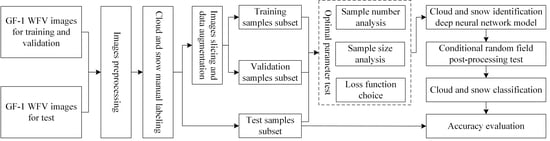
2. Data and Methodology

2.1. GF-1 WFV Data

The high-resolution remote sensing image used in this paper is the Wide Field View (WFV) sensor data of China Gaofen-1 (GF-1) satellite. The orbit height of GF-1 satellite is 645 km. The image of WFV sensor contains four bands of red, green, blue and near-infrared, with a spatial resolution of 16 m and a width of 800 km. The specific parameters of GF-1 WFV are shown in

Table 1. GF-1 WFV parameters.

Sensor	Band	Band Range (μm)	Radiometric Resolution (Bit)	Spatial Resolution (m)
Wide Field View (WFV)	1	0.45~0.52	10	16
	2	0.52~0.59
	3	0.63~0.69
	4	0.77~0.89

. The specific data used in this paper are listed in

Table 2. List of data used in the paper.

Number	Sensor	Scene Serial Number	Imaging Time	Remarks
1	WFV1	6013180	22 January 2019	Model training and validation images
2	WFV3	8348146	31 October 2020
3	WFV4	6252997	29 March 2019
4	WFV3	5848541	8 December 2018
5	WFV4	5416209	16 August 2018
6	WFV3	7050682	5 November 2019
7	WFV2	8155402	16 September 2020
8	WFV1	4330375	13 November 2017	Model test images
9	WFV3	6658981	18 July 2019
10	WFV1	4314475	9 November 2017

. A total of ten GF-1 WFV data images from November 2017 to October 2020 were used. Among them, seven images were used for model training and validation, and the other three images were used for model testing. Radiometric calibration and atmospheric correction of these images was performed before sample labeling and model training.

2.2. Sample Labeling

Since cloud and snow cover vary frequently with time, it is necessary to label samples by manual vectorization. The labeling categories are divided into three categories, which are snow, cloud and background. Considering the difficulty and limited accuracy of manual labeling for snow in shadows, both mountain shadows and cloud shadows are annotated as background samples in order to not affect the accuracy of model training and testing. Firstly, the regions with relatively concentrated cloud and snow in the seven training and validation images are manually vectorized and labeled, and the labeled regions are cropped to a total of 2000 pieces of sample with 256 × 256 pixel size and four bands. Secondly, in order to avoid overfitting of the model due to the small amount of training samples and to improve the robustness of the model, in this paper, the data augmentation methods such as rotation, Blur transform and adding Gaussian noise are used to increase the amount of samples. Here, the above 2000 pieces of sample are expanded to 10,000. These 10,000 pieces of sample with a size of 256 × 256 × 4 pixels are all used as the training and validation set of the cloud and snow identification neural network model, in which the training subset accounts for 75% and the validation subset accounts for 25%. At the same time, for the other three test images, the regions with relatively concentrated cloud and snow are only manually vectorized and annotated, without cropping and data augmentation, and the annotation results are directly used as the test data for the accuracy evaluation. Some labeled data are shown in Figure 1.

2.3. DeepLab V3+ Model

DeepLab v3+ is the latest model in Google’s DeepLab series, and the model structure is shown in Figure 2. Compared with the DeepLab v3 model, its biggest feature is to replace most of the convolutions in the network with dilated convolutions, which enhances the ability of the model to extract dense features of images without increasing the amount of calculated parameters while obtaining a larger sensory domain.

The skeleton network of the DeepLab v3+ encoder part is an Xception network with atrous convolution. The network is developed based on Inception v3+, and the model structure is similar to the residual connection in ResNet. It is considered that spatial correlations and inter-channel correlations should be dealt with separately. Therefore, Depthwise separable convolution is used to divided the ordinary convolution into Depthwise convolution and Pointwise convolution. Deepwise convolution performs spatial convolution only for each channel eigenvalue independently, and Pointwise convolution only performs for different channel eigenvalues of each pixel, which can reduce parameters and computation, and reduce computational complexity and maintain similar performance [21]. Xception replaces all the maximum pooling layer operations with depth separation convolution with step size without modifying the entry flow, middle flow and exit flow structure of the traditional entry flow network. Finally, the same as DeepLab v3, the Atrous Spatial Pyramid Pooling (ASPP), is used to extract the context information of remote sensing images at four different scales in four different sensory domains, so as to achieve robust segmentation and thus improve the segmentation effect.

The decoding part of DeepLab v3+ model refers to the step-skipping connection mode of the Full Coiler Network (FCN), and fuses the low-level detail features in the encoder part with the high-level features’ output from the encoder part by convolutional dimension reduction. Then the feature fusion image is restored to the original image size using 1 × 1 convolution and bilinear interpolation upsampling method. Finally, the Softmax activation function is also used to classify each pixel.

2.4. Loss Function

In the training process of neural network, the loss function is used to calculate the difference between the model predicted value and the true label value, to optimally adjust the parameters and training process in the model, and to evaluate the training results of the model. It is inversely proportional to the accuracy of the model. Cross Entropy Loss (CE) is generally used as the loss function in image segmentation, examines each pixel one by one, but is prone to fitting difficulties caused by too small loss when the sample amount of different types is extremely unbalanced. In medical image processing, because the anatomical structure of interest usually occupies only a small area in the scanned image, the Dice loss function is proposed in V-Net [22] to increase the weight of the foreground area, which prevents the model from falling into the local minimum of the loss function during the training process. In the field of target detection, the Focal loss function [23] is usually used to solve the problem of severe imbalance in the proportion of positive and negative samples. In the case of unbalanced categories, it can make the loss smaller for samples with high prediction probability and the loss larger for samples with low prediction probability, thus strengthening the attention of the model on the positive samples. In this study, because there are many more background samples and more cloud samples than snow samples in the labeled dataset, the Focal function is chosen as the loss function, which can effectively solve the problem that the proportion of foreground samples is too small. The formulas are as follows:

$$CrossEntropy:E=-{{\displaystyle \sum }}_{i=1}^n{P}_i\log \left(Q_i\right),$$

(1)

$$Dice:E=1-\frac{{{\displaystyle \sum }}_{i=1}^n{P}_i{Q}_i+\epsilon }{{{\displaystyle \sum }}_{i=1}^n{P}_i+Q_i+\epsilon }-\frac{{{\displaystyle \sum }}_{i=1}^n(1-P_i)\left(1-Q_i\right)+\epsilon }{{{\displaystyle \sum }}_{i=1}^{n}2-P_i-Q_i+\epsilon },$$

(2)

$$Focal:E=-{{\displaystyle \sum }}_{i=1}^n{\left(1-Q_i\right)}^{\gamma }{P}_i\log \left(Q_i\right),$$

(3)

where n is the number of categories; P_i is the true probability distribution; Q_i is the model prediction probability distribution; the value of ε in the Dice loss function formula is generally one to avoid the gradient explosion caused by denominator being zero or too small. γ in the Focal loss function is the parameter that controls the orientation of the sample tendency, generally takes the value of zero to five. In this paper, a triple classification (cloud, snow, background) problem is discussed, so n is three, P_i and Q_i are 256 × 256 matrices, where P_i is the sample label image, Qi is the model classification image.

2.5. Conditional Random Field

The conditional random field model is a probabilistic graph model proposed by Lafferty et al. (2001) [24]. It combines the unary potential energy of a single pixel and the pairwise potential energy between neighboring pixels, so that the spatial pixels are assigned to the same label. It is usually applied to smooth the segmentation maps with edge noise. However, its structure cannot model the pixels far apart and is prone to over-smoothing of target object boundaries. To solve this problem, Krähenbühl et al. (2011) proposed the concept of fully connected CRF based on CRF [25]. In fully connected CRF, the energy of predicted label value X is defined as

$$E\left(X\right)={{\displaystyle \sum }}_i{\psi }_u(x_i)+{{\displaystyle \sum }}_{i<j}{\psi }_p(x_i,x_j),$$

(4)

where, i, j represent pixels; x_i and x_j are the labels assigned to pixels i and j, respectively; ${\psi }_u\left(x_i\right)$ represents unary potential energy; ${\psi }_p\left(x_i,x_j\right)$ represents pairwise potential energy. The unary potential energy represents the class probability distribution obtained from independent prediction of each pixel i in the classification image to be improved in accuracy, which contains much noise and is discontinuous. The pairwise potential energy represents a fully connected graph that connects all pixels of the image and classifies pixels with the same properties into the same category as much as possible. When the energy E(X) of fully connected CRF is smaller, the predicted pixel category label X is more accurate. The average field approximation is generally used to iterate and find the minimum energy function so as to obtain the result of improved boundary accuracy. In this paper, the pixel category distribution probability map output from DeepLab v3+ neural network model is taken as unary potential energy, and the original high-resolution remote sensing image is taken as pairwise potential energy.

2.6. Evaluation Indicators

In order to explore the advantages and disadvantages of different neural network models in cloud and snow identification, the accuracy criteria in this paper are Mean Intersection over Union (MIoU) and the Mean Pixel Accuracy (MPA) [26,27]. The MIoU is the result of averaging the ratio of the intersection set to the union set of the true values derived from each class of prediction results, which can represent the accuracy of each class. MPA is the result of averaging the proportion of correctly classified pixels for each class. Both evaluation indicators take values in the range of zero to one, with closer to one representing better segmentation. Both of them are commonly used criteria to verify the accuracy of neural network model. Therefore, these two indicators are used as quantitative research criteria in this paper. The expressions are as follows

$$\mathrm{MIoU}=\frac{1}{K+1}{{\displaystyle \sum }}_{I=0}^K(\frac{n_{ii}}{{{\displaystyle \sum }}_{j=0}^K\left(n_{ij}+n_{ji}\right)-n_{ii}}),$$

(5)

$$\mathrm{MPA}=\frac{1}{K+1}{{\displaystyle \sum }}_{I=0}^K(\frac{n_{ii}}{{{\displaystyle \sum }}_{j=0}^K{n}_{ij}}),$$

(6)

where there are a total of K + 1 label categories (K classes of objects and one other category) in the classified image; n_ii is the number of correct predictions of class i; n_ij is the number of class i pixels predicted as class j; and n_ji is the number of class j pixels predicted as class i.

2.7. Experimental Environment

The experimental platform in this paper is an Inter (R) Core (TM) i7-9700F @ 3.0 GHz CPU, NVIDIA GeForce RTX 2060 SUPPER 8 GB graphics card and 16.0 GB running memory. In terms of software environment, Python is used as the main programming language under Windows 10 system, and the high-performance computing library CUDA11.0 for the display card is installed. The deep learning framework adopts TensorFlow 2.5.0 and Keras 2.3.1. In the training process, Adam is selected as the optimizer to update the network gradient, and Softmax activation function is used to classify each pixel. The learning rate is set to 0.001, the batch size is 5 and the iteration number (epoch) is 200.

3. Experiments and Results

The number of samples, sample size and loss function have a certain impact on the accuracy of the semantic segmentation neural network model, and the post-processing work will also affect the identification results. Generally, the smaller the sample number, the easier it is to cause overfitting. If the sample size is too small, it is impossible to learn to obtain more spatial semantic information, and it is easy to misclassify snow and cloud with similar spectral characteristics; if the sample size is too large, the model training time increases and the generalization ability decreases. At the same time, the model training accuracy will be different while using the different loss functions. Therefore, this study analyzed the effects of different sample numbers, sample sizes and loss functions on the DeepLab v3+ model for cloud and snow identification, as well as the impact of CRF post-processing on the accuracy of cloud and snow identification, so as to provide a reference for the optimal parameter selection of the semantic segmentation neural network model for cloud and snow identification.

3.1. Sample Number Analysis

In order to investigate the optimal number of samples required for model training, 2000, 5000 and 10,000 samples were randomly taken from the 10,000 training and validation sets prepared above, respectively, and input to the DeepLab v3+ model, in turn, for training. Among them, 2000 samples were directly taken from those training and validation samples without data augmentation. The batch size was 5, epoch was 200 and neural network models for cloud and snow identification trained by different sample numbers were obtained. The curves of loss value and the accuracy of model training with each batch are shown in Figure 3.

It can be seen from Figure 3 that the larger the number of samples, the smaller the fluctuation in the training loss value and training accuracy, and the higher the stability of the model. When the number of samples is 2000, the training loss value and training accuracy fluctuate greatly, and the model stability is very low. When the number of samples is 5000 and the iteration times is more than 100, the training loss value and training accuracy are comparable to those when the number of samples is 10,000, but the stability of the model is still insufficient. When the number of samples is 10,000 and the time of iterations reaches 170, the model training accuracy is high and the stability is strong. Therefore, the number of 10,000 training samples is more suitable for training the cloud and snow identification model with high accuracy and stability.

Figure 4 shows the prediction maps for the test data by using the models with different sample numbers. The prediction accuracies are shown in

Table 3. Comparison of model test accuracy under different sample numbers.

Sample Number	Snow IoU	Cloud IoU	MIoU	Snow PA	Cloud PA	MPA
2000	0.761	0.647	0.756	0.827	0.760	0.845
5000	0.766	0.619	0.750	0.808	0.810	0.857
10,000	0.804	0.757	0.816	0.891	0.934	0.918

. As seen in Figure 4, when sample numbers are 2000 and 5000, there are more misclassified cloud and snow pixels. Snow IoU, Cloud IoU, Snow PA and Cloud PA, as well as MIoU and MPA, are relatively low. In addition, compared with the number of 2000 samples, the prediction accuracy of the model trained by 5000 samples has not improved, and even Cloud IoU, MIoU and Snow PA have some reduction. When the number of samples is 10,000, the misclassified pixels of cloud and snow are significantly reduced. The MIoU and MPA are 0.816 and 0.918, respectively, which are 0.066 and 0.061 higher than the accuracy of 5000 samples. This is a significant improvement. In summary, the model training accuracy, stability and prediction accuracy are optimal when the number of samples is 10,000.

3.2. Sample Size Analysis

In order to analyze the appropriate sample size for cloud and snow identification in the GF-1 WFV image using the DeepLab v3+ model, the previous 10,000 samples of 256 × 256 size were cut into 10,000 samples of 64 × 64 size and 10,000 samples of 128 × 128 size, respectively. These samples with different sizes were input to the DeepLab v3+ model for training in turn. The loss function was set to the Focal function, the batch size was set to 5 and the epoch was set to 200. The variation curves of the loss value and accuracy of model training with the iteration times are shown in Figure 5.

As seen in Figure 5, in the early stage of training, the larger the sample size, the faster the fitting speed is. As the number of iterations increases, the differences in model training loss between different sample sizes gradually decrease, as does the difference in model training accuracy. However, within 200 iterations, the training loss value of the model trained by the sample sizes of 256 × 256 is always better than those trained by the sample sizes of 64 × 64 and 128 × 128; the training accuracy of the model is always higher than that of the sample sizes of 64 × 64 and 128 ×128 accuracy; and the model stability is better when the sample sizes is 256 × 256, and the model tends to be stable when the number of iterations reaches 170.

Figure 6 shows the prediction maps for the test data by using models with different sample sizes, and the prediction accuracies are shown in

Table 4. Comparison of model test accuracy under different sample sizes.

Sample Size	Snow IoU	Cloud IoU	MIoU	Snow PA	Cloud PA	MPA
64 × 64	0.761	0.630	0.754	0.866	0.795	0.862
128 × 128	0.764	0.599	0.748	0.877	0.691	0.838
256 × 256	0.804	0.757	0.816	0.891	0.934	0.918

. As seen in Figure 6 and Table 4, when the training sample sizes are 64 × 64 and 128 × 128, the cloud and snow are seriously misclassified in the prediction maps, and Snow IoU, Cloud IoU, Snow PA and Cloud PA, as well as MIoU and MPA are relatively low. The MIoU and MPA are only 0.754 and 0.862, the prediction accuracy of the 128 × 128 size is not improved compared with that of the 64 × 64 size, and the Cloud IoU, MIoU, Cloud PA and MPA are even reduced to a certain extent; in addition, the classification map of 128 × 128 size shows serious slicing traces. When the training sample size is 256 × 256, the prediction accuracy of the model is greatly improved, and the misclassified pixels of cloud and snow are significantly reduced. The MIoU and MPA reach 0.816 and 0.918, respectively, and the Cloud PA even reaches 0.934. It can be seen that the appropriate increase in sample size can reduce some misclassification pixels and improve the accuracy of the model, but at the same time, it also makes the model training slower and less efficient. In summary, when the sample size is 256 × 256, the training accuracy, stability and prediction accuracy of the model are relatively better.

3.3. Selection of Loss Function

To investigate the accuracy differences of different loss functions on the DeepLab v3+ model for cloud and snow identification, the CE loss function, Dice loss function and Focal loss function were selected, respectively, in the experiment, and 10,000 pieces of 256 × 256 size samples were input to train the DeepLab v3+ models for cloud and snow identification. The batch size was set to five, and the epoch was 200. The changes in training loss value and training accuracy were recorded, as shown in Figure 7.

It can be seen from Figure 7 that the training loss curve of Dice converges faster and the loss value is smaller in the whole process of training, but the training accuracies of these three loss functions are relatively close. In terms of the stability of training accuracy, the CE function has the most stable performance, but the difference with the Dice and Focal functions is not obvious.

Figure 8 shows the prediction maps for the test data by using models under different loss functions, and the prediction accuracies are shown in

Table 5. Comparison of model test accuracy under different loss functions.

Loss Function	Snow IoU	Cloud IoU	MIoU	Snow PA	Cloud PA	MPA
CE	0.759	0.595	0.741	0.846	0.683	0.827
Dice	0.777	0.763	0.803	0.845	0.917	0.899
Focal	0.805	0.757	0.816	0.891	0.934	0.918

. From Figure 8 and Table 5, it can be seen that the model using the CE loss function has more snow pixels misclassified as cloud, and the slicing traces are obvious. Compared with the Dice function and Focal function, the prediction accuracy of the model using the CE function is also the lowest, with MIoU and MPA only 0.741 and 0.827, respectively. The model accuracy using the Dice or Focal loss functions improves somewhat. In particular, because the Focal function increases the focus of the model on snow and cloud samples, the problem of an unbalanced number of samples of each category in the training samples set improves. In the model prediction maps, the misclassified pixels of cloud and snow are significantly reduced, and the model prediction accuracy is significantly improved. The Cloud PA reaches 0.934 and the Snow PA reaches 0.891. The MIoU and MPA are higher than those of CE and the Dice loss function. In summary, the training accuracies of the models using the CE, Dice and Focal functions are comparable, but the model using the Focal loss function has higher prediction accuracy and stronger generalization ability.

3.4. Conditional Random Field Post-Processing

In order to investigate the effectiveness of CRF post-processing on the accuracy improvement of the DeepLab v3+ model for cloud and snow classification, the CRF model is used to post-process the cloud and snow classification results of DeepLab v3+ model. The cloud and snow classification map predicted by the DeepLab v3+ model on the test data is taken as the univariate potential energy of the conditional random field, and the GF-1 WFV image is used as the unary potential energy. The mean field approximation method is used to iteratively find the minimum energy function E(X). The smaller E(X) is, the more accurate the predicted pixel class label X is, resulting in a classification map with improved boundary accuracy, as shown in Figure 9.

Figure 9 shows the comparison of prediction maps before and after CRF post-processing, and Figure 10 shows the comparison of their local details before and after post-processing. From Figure 9 and Figure 10, it is obvious that the DeepLab v3+ model misidentifies some isolated small patches of snow as clouds; and the boundaries of the snow are smoother and different from the true snow cover. In addition, the semantic segmentation neural network classifies the image after slicing, and then splices the classified slices. Different slices will take global consideration, respectively, so that different prediction results are generated at the boundaries of adjacent slices, thus leading to some slicing traces in the final spliced classification map. After the CRF post-processing, the misclassified clouds are correctly identified as snow again, and the boundaries of the snow cover are also finer and more closely match the true ground objects; at the same time, the slicing traces and isolated small patches are also eliminated.

In order to quantitatively analyze the effectiveness of CRF post-processing on the accuracy improvement of cloud and snow identification, The MIoU and MPA of the classification maps before and after CRF post-processing were calculated respectively and are shown in

Table 6. Comparison results of different models.

Model	Snow IoU	Cloud IoU	MIoU	Snow PA	Cloud PA	MPA
DeepLab v3+	0.805	0.757	0.816	0.891	0.934	0.918
DeepLab v3+ and CRF	0.829	0.787	0.836	0.890	0.997	0.941

. It can be seen that Snow IoU, Cloud IoU and Cloud PA, as well as MIoU and MPA, are effectively improved, where MIoU and MPA are improved from 0.816 and 0.918 to 0.836 and 0.941, respectively, and the improvement compared with no post-processing is 0.020 and 0.023, respectively. In summary, the combined model of DeepLab v3+ and CRF can effectively correct the misclassification problems such as blurred boundaries, slicing traces and isolated small patches, thus further improving the cloud and snow identification accuracy.

4. Discussion

When conducting image semantic segmentation experiments, it can be better to use authoritative public datasets. Tian et al. (2019) summarized some common public datasets for image semantic segmentation [28]. PASCAL VOC 2012 is one of the public standard datasets commonly used in the field of computer vision [29], and many scholars have studied the effectiveness and generalization of models using public datasets [30,31,32]. However, due to the frequent temporal changes in snow and cloud, there are few publicly available high spatial resolution cloud and snow labeling datasets. Therefore, the training datasets used in this paper are all completed by manual visual annotation. Since the annotation of deep learning datasets is time-consuming and labor-intensive, and the number of samples is relatively insufficient, many scholars have used data augmentation methods to increase the amount of sample data, including operations horizontal flips, vertical flips, diagonal mirroring and random scaling [33,34]. In this paper, various data augmentation operations are also used to increase the sample number of the labeled dataset, eliminate the overfitting caused by the small number of samples and improve the robustness of the model. The experimental results of different sample numbers in Section 3.1 also demonstrate that increasing the sample number by data augmentation can improve the identification accuracy of the model.

Wieland et al. (2019) achieved an accuracy of 0.89 for cloud and snow identification in multi-spectral satellite images based on the improved U-Net convolutional neural network [35]. The Fmask 4.0 algorithm proposed by Qiu et al. (2019) has an overall accuracy of 0.924 for cloud identification in Landsat 4–7 images [36]. In the tests of this paper, the accuracy for cloud and snow identification using only the DeepLab v3+ neural network is 0.918. However, as seen from the prediction maps above, there are still some misclassification problems such as blurred boundaries, slicing traces and isolated small patches. The CRF model can capture fine-grained information and infer the output class of target pixels by combining the target pixels with the nearby pixels, which is not achieved by the convolutional neural network focusing on local information. Some scholars previously used the CRF to extract the target features in remote sensing images, and the results show that the CRF model can improve the accuracy of the segmentation results [37,38]. In this paper, CRF post-processing for the predicted maps of the DeepLab v3+ model is carried out to further improve the pixel accuracy. The accuracy reaches 0.941, which is 0.023 higher than the accuracy before CRF post-processing, and 0.051 and 0.017 higher than the accuracy of the U-Net and Fmask 4.0 models, respectively, and the misclassification problems of blurred boundaries, slicing traces and isolated small patches are corrected. This further demonstrates that the CRF post-processing method can effectively optimize the boundary of cloud and snow and improve the accuracy of the segmentation. Therefore, it is feasible to combine the DeepLab v3+ and CRF models for cloud and snow identification in high-resolution remote sensing images.

5. Conclusions

Aimed at the problem that it is difficult to use the snow index algorithm to identify cloud and snow in high-resolution remote sensing images lacking the short-wave infrared band, and the problem that the semantic segmentation neural network model is prone to producing blurred boundaries, slicing traces and isolated small patches, in this paper, the feasibility and the optimal parameter selection of the DeepLab v3+ and CRF combined model for cloud and snow identification in high-resolution remote sensing images are explored through the comparative experimental analysis of different sample numbers, sample sizes, loss functions and CRF post-processing using GF-1 WFV images. The main conclusions are as follows:

(1)

The DeepLab v3+ model is used to identify cloud and snow in a GF-1 WFV image. When the number of samples is 10,000, the sample size is 256 × 256, and the loss function is the Focal function, the model has the optimal accuracy and strong stability, where the MIoU and the MPA reach 0.816 and 0.918, respectively.

(2)

For the cloud and snow identification, CRF post-processing can significantly improve the misclassification problems such as blurred boundaries, slicing traces and isolated small patches caused by the semantic segmentation of neural network model. Compared with the prediction maps without post-processing, the prediction accuracy after CRF post-processing is effectively improved. The MIoU and MPA are improved to 0.836 and 0.941, respectively, which proves the effectiveness of the post-processing method.

(3)

The DeepLab v3+ and CRF combined model for cloud and snow identification in a high-resolution remote sensing image has high accuracy and strong feasibility. The conclusions can provide a technical reference for the application of deep learning algorithms in high-resolution snow mapping and hydrological application.

The sample accuracy is a key factor affecting the prediction results of the semantic segmentation model. The manual labeling accuracy of cloud and snow samples is greatly affected by human factors; in particular, the manual labeling of snow in shadows is more difficult and has limited accuracy. Therefore, this paper treats both mountain shadows and cloud shadows as background categories. This treatment has certain limitations, which reduces the accuracy of cloud and snow identification. Therefore, how to reduce the influence of human factors on the accuracy of samples and improve the accuracy of cloud and snow identification, especially to improve the accuracy of snow identification in shadow areas, is the direction of further research. The authors will next try to use a weakly supervised learning method to identify cloud and snow in high-resolution remote sensing images to reduce the impact of human factors.

References

1. Shi, Y.; Cheng, G. The Cryosphere and Global Change. Bull. Chin. Acad. Sci. 1991, 4, 287–291. [Google Scholar] [CrossRef]
2. Qin, D.; Zhou, B.; Xiao, C. Progress in studies of cryospheric changes and their impacts on climate of China. Acta Meteorol. Sin. 2014, 72, 869–879. [Google Scholar] [CrossRef]
3. Yao, T.; Qin, D.; Shen, Y.; Zhao, L.; Wang, N.; Lu, A. Cryospheric changes and their impacts on regional water cycle and ecological conditions in the Qinghai-Tibetan Plateau. Chin. J. Nat. 2013, 35, 179–186. [Google Scholar]
4. Wu, H. Research of Cloud and Snow Discrimination from Multispectral High-Resolution Satellite Images. Master’s Thesis, Wuhan University, Wuhan, China, 2018. [Google Scholar]
5. Ying, Q.; Yang, Y.; Xu, W. Research on Distinguishing between Cloud and Snow with NOAA Images. Plateau Meteorol. 2002, 21, 526–528. [Google Scholar]
6. Ding, H.; Ma, L.; Li, Z.; Tang, L. Automatic Identification of Cloud and Snow based on Fractal Dimension. Remote Sens. Technol. Appl. 2013, 28, 52–57. [Google Scholar]
7. Joshi, P.P.; Wynne, R.H.; Thomas, V.A. Cloud detection algorithm using SVM with SWIR2 and tasseled cap applied to Landsat 8. Int. J. Appl. Earth Obs. Geoinf. 2019, 82, 101898. [Google Scholar] [CrossRef]
8. Ghasemian, N.; Akhoondzadeh, M. Introducing two Random Forest based methods for cloud detection in remote sensing images. Adv. Space Res. 2018, 62, 288–303. [Google Scholar] [CrossRef]
9. Long, J.; Shelhamer, E.; Darrell, T. Fully convolutional networks for semantic segmentation. In Proceedings of the 2015 IEEE Conference on Computer Vision and Pattern Recognition (CVPR), Boston, MA, USA, 7–12 June 2015; pp. 3431–3440. [Google Scholar]
10. Maggiori, E.; Tarabalka, Y.; Charpiat, G.; Alliez, P. Convolutional neural networks for large-scale remote-sensing image classification. IEEE Trans. Geosci. Remote Sens. 2016, 55, 645–657. [Google Scholar] [CrossRef]
11. Liu, W. Cloud and Snow Classification in Plateau Area Based on Deep Learning Algorithms. Master’s Thesis, Nanjing University of Information Science and Technology, Nanjing, China, 2019. [Google Scholar]
12. Wang, J.; Li, J.; Zhou, H.; Zhang, X. Typical element extraction method of remote sensing image based on Deeplabv3+ and CRF. Comput. Eng. 2019, 45, 260–265, 271. [Google Scholar] [CrossRef]
13. Guo, X.; Chen, Y.; Liu, X.; Zhao, Y. Extraction of snow cover from high-resolution remote sensing imagery using deep learning on a small dataset. Remote Sens. Lett. 2020, 11, 66–75. [Google Scholar] [CrossRef]
14. Wang, Y.; Su, J.; Zhai, X.; Meng, F.; Liu, C. Snow Coverage Mapping by Learning from Sentinel-2 Satellite Multispectral Images via Machine Learning Algorithms. Remote Sens. 2022, 14, 782. [Google Scholar] [CrossRef]
15. Zhang, G.; Gao, X.; Yang, Y.; Wang, M.; Ran, S. Controllably Deep Supervision and Multi-Scale Feature Fusion Network for Cloud and Snow Detection Based on Medium- and High-Resolution Imagery Dataset. Remote Sens. 2021, 13, 4805. [Google Scholar] [CrossRef]
16. Nambiar, K.G.; Morgenshtern, V.I.; Hochreuther, P.; Seehaus, T.; Braun, M.H. A Self-Trained Model for Cloud, Shadow and Snow Detection in Sentinel-2 Images of Snow- and Ice-Covered Regions. Remote Sens. 2022, 14, 1825. [Google Scholar] [CrossRef]
17. Park, J.; Shin, C.; Kim, C. PESSN: Precision Enhancement Method for Semantic Segmentation Network. In Proceedings of the 2019 IEEE International Conference on Big Data and Smart Computing (BigComp), Tokyo, Japan, 4 April 2019; pp. 1–4. [Google Scholar]
18. Jeong, H.G.; Jeong, H.W.; Yoon, B.H.; Choi, K.S. Image Segmentation Algorithm for Semantic Segmentation with Sharp Boundaries using Image Processing and Deep Neural Network. In Proceedings of the 2020 IEEE International Conference on Consumer Electronics—Asia (ICCE-Asia), Seoul, Korea, 1 November 2020; pp. 1–4. [Google Scholar]
19. Sun, X.; Shi, A.; Huang, H.; Mayer, H. BAS4Net: Boundary-Aware Semi-Supervised Semantic Segmentation Network for Very High Resolution Remote Sensing Images. IEEE J. Sel. Top. in Appl. Earth Obs. Remote Sens. 2020, 13, 5398–5413. [Google Scholar] [CrossRef]
20. Li, K. Semi-supervised Classification of Hyperspectral Images Combined with Convolutional Neural Network and Conditional Random Fields. Master’s Thesis, China University of Geosciences, Beijing, China, 2021. [Google Scholar]
21. Chen, L.; Zhu, Y.; Papandreou, G.; Schrof, F.; Adam, H. Encoder-decoder with atrous separable convolution for semantic image segmentation. In Proceedings of the European conference on computer vision (ECCV), Munich, Germany, 8–14 September 2018; pp. 801–818. [Google Scholar]
22. Zhu, Z.; Liu, C.; Yang, D.; Yuille, A.; Xu, D. V-NAS: Neural Architecture Search for Volumetric Medical Image Segmentation. In Proceedings of the 2019 IEEE International Conference on 3D Vision (3DV), Québec City, QC, Canada, 16–19 September 2019; pp. 240–248. [Google Scholar]
23. Lin, T.Y.; Goyal, P.; Girshick, R.; He, K.; Dollar, P. Focal loss for dense object detection. In Proceedings of the 2017 IEEE International Conference on Computer Vision (ICCV), Venice, Italy, 22–29 October 2017; pp. 2999–3007. [Google Scholar]
24. Lafferty, J.; Mccallum, A.; Pereira, F. Conditional Random Fields: Probabilistic Models for Segmenting and Labeling Sequence Data. In Proceedings of the Eighteenth International Conference on Machine Learning (ICML ‘01), San Francisco, CA, USA, 28 June–1 July 2001; pp. 282–289. [Google Scholar]
25. Krähenbühl, P.; Koltun, V. Efficient inference in fully connected crfs with gaussian edge potentials. In Proceedings of the 24th International Conference on Neural Information Processing Systems (NIPS’11), Red Hook, NY, USA, 12–15 December 2011; pp. 109–117. [Google Scholar]
26. Alberto, G.G.; Sergio, O.E.; Sergiu, O.; Victor, V.M.; Jose, G.R. A Review on Deep Learning Techniques Applied to Semantic Segmentation. arXiv 2017, arXiv:1704.06857. [Google Scholar]
27. Jing, Z.W.; Guan, H.Y.; Peng, D.F.; Yu, Y.T. Survey of Research in Image Semantic Segmentation Based on Deep Neural Network. Comput. Eng. 2020, 46, 1–17. [Google Scholar] [CrossRef]
28. Tian, X.; Wang, L.; Ding, Q. Review of image semantic segmentation based on deep learning. J. Softw. 2019, 30, 440–468. [Google Scholar] [CrossRef]
29. Everingham, M.; Eslami, S.M.; Gool, L.; Williams, C.K.; Winn, J.; Zisserman, A. The pascal visual object classes challenge: A retrospective. Int. J. Comput. Vis. 2015, 111, 98–136. [Google Scholar] [CrossRef]
30. Chen, L.C.; Papandreou, G.; Kokkinos, I.; Murphy, K.; Yuille, A.L. Deeplab: Semantic image segmentation with deep convolutional nets, atrous convolution, and fully connected CRFs. IEEE Trans. Pattern Anal. Mach. Intell. 2018, 40, 834–848. [Google Scholar] [CrossRef]
31. Chen, L.C.; Papandreou, G.; Schroff, F.; Adam, H. Rethinking atrous convolution for semantic image segmentation. arXiv 2017, arXiv:1706.05587. [Google Scholar]
32. Meng, J.; Zhang, L.; Cao, Y.; Zhang, L.; Song, Q. Research on optimization of image semantic segmentation algorithms based on Deeplab v3+. Laser Optoelectron. Prog. 2022, 59, 161–170. [Google Scholar]
33. Yan, Q.; Liu, H.; Zhang, J.; Sun, X.; Xiong, W.; Zou, M.; Xia, Y.; Xun, L. Cloud Detection of Remote Sensing Image Based on Multi-Scale Data and Dual-Channel Attention Mechanism. Remote Sens. 2022, 14, 3710. [Google Scholar] [CrossRef]
34. Zhao, W.; Li, M.; Wu, C.; Zhou, W.; Chu, G. Identifying Urban Functional Regions from High-Resolution Satellite Images Using a Context-Aware Segmentation Network. Remote Sens. 2022, 14, 3996. [Google Scholar] [CrossRef]
35. Wieland, M.; Li, Y.; Martinis, S. Multi-sensor cloud and cloud shadow segmentation with a convolutional neural network. Remote Sens. Environ. 2019, 230, 111203. [Google Scholar] [CrossRef]
36. Qiu, S.; Zhu, Z.; He, B.B. Fmask 4.0: Improved cloud and cloud shadow detection in Landsats 4–8 and Sentinel-2 imagery. Remote Sens. Environ. 2019, 231, 111205. [Google Scholar] [CrossRef]
37. Zhu, Q.; Li, Z.; Zhang, Y.; Li, J.; Du, Y.; Guan, Q.; Li, D. Global-Local-Aware conditional random fields based building extraction for high spatial resolution remote sensing images. Natl. Remote Sens. Bull. 2021, 25, 1422–1433. [Google Scholar]
38. He, Q.; Zhao, L.; Kuang, G. SAR airport runway extraction method based on semantic segmentation model and conditional random field. Mod. Radar. 2021, 43, 91–100. [Google Scholar] [CrossRef]
Figure 1. Examples of labeled dataset. Subfigures (af) are eight pairs of cloud and snow labels on different dates, each with remote sensing image on the left and corresponding labeled image on the right.
Remotesensing 14 04880 g001
Figure 2. DeepLab v3+ structure [21]. It adopts encoder-decoder structure. The arrows in the figure represent the data flow. The red, blue and gray in the prediction map represent different ground objects.
Remotesensing 14 04880 g002
Figure 3. The change curve of training loss value with the iterations times (a) and the change curve of training accuracy with the iterations times (b) under different sample numbers.
Remotesensing 14 04880 g003
Figure 4. Comparison of cloud and snow identification under different sample numbers. The three columns of subfigures (ac) represent the original image, the label image, and the prediction maps under the sample number of 2000, 5000, and 10,000 at three different dates, respectively.
Remotesensing 14 04880 g004
Figure 5. The change curve of training loss value with the iterations times (a) and the change curve of training accuracy with the iterations times (b) under different sample sizes.
Remotesensing 14 04880 g005
Figure 6. Comparison of cloud and snow identification under different sample sizes. The three columns of subfigures (ac) represent the original image, the label image, and the prediction maps under the sample size of 64 × 64, 128 × 128, and 256 × 256 at three different dates, respectively.
Remotesensing 14 04880 g006
Figure 7. The change curve of training loss value with the iterations times (a) and the change curve of training accuracy with the iterations times (b) under different loss functions.
Remotesensing 14 04880 g007
Figure 8. Comparison of cloud and snow identification under different loss functions. The three columns of subfigures (ac) represent the original image, the label image, and the prediction maps under CE, Dice, and Focal loss functions at three different dates, respectively.
Remotesensing 14 04880 g008
Figure 9. Comparison of cloud and snow identification between DeepLab v3+ and CRF post-processing. The three columns of subfigures (ac) represent the original image, the label image, the DeepLab v3+ prediction map and the prediction map of DeepLab v3+ & CRF at three different dates, respectively.
Remotesensing 14 04880 g009
Figure 10. Post-processing cloud and snow identification comparison map (local details). The four lines of subfigures (ad) represent the significant improvements of isolated small patches, blurred boundaries and slicing traces, respectively. The inside black rectangles show the corresponding areas where improved.
Remotesensing 14 04880 g010