Article

Factors Controlling a Synthetic Aperture Radar (SAR) Derived Root-Zone Soil Moisture Product over The Seward Peninsula of Alaska

1
Earth and Environmental Sciences, Los Alamos National Laboratory, Los Alamos, NM 87545, USA
2
International Arctic Research Center, University of Alaska Fairbanks, Fairbanks, AK 99775, USA
*
Author to whom correspondence should be addressed.
Remote Sens. 2022, 14(19), 4927; https://doi.org/10.3390/rs14194927
Submission received: 18 August 2022 / Revised: 18 September 2022 / Accepted: 22 September 2022 / Published: 2 October 2022

Abstract

:
Root-zone soil moisture exerts a fundamental control on vegetation, energy balance, and the carbon cycle in Arctic ecosystems, but it is still not well understood in vast, remote, and understudied regions of discontinuous permafrost. The root-zone soil moisture product (30 m resolution) used in this analysis was retrieved from a time-series P-Band (420–440 MHz) synthetic aperture radar (SAR) backscatter observations (August 2017 & October 2017). While similar approaches have been taken to retrieve surface (0 cm to 5 cm) soil moisture from L-Band (1.2 GHz) SAR backscatter, this is one of the first known attempts at reaching the root-zone in permafrost regions. Here, we analyze secondary factors (excluding primary factors, such as precipitation) controlling summer (August) soil moisture at depths of 6 cm, 12 cm, and 20 cm over a 4500 km2 area on the Seward Peninsula of Alaska. Using a random forest model, we quantify the impact of topography, vegetation, and meteorological factors on soil moisture distributions. In developing the random forest model, we explore a variety of feature scales (30 m, 60 m, 90 m, 120 m, 180 m, and 240 m), tune hyperparameters (the structure of individual decision trees making up the ensemble including the number and depth of trees), and perform the final feature selection using cross-validated recursive feature elimination. Results suggest that root-zone soil moisture on the Seward Peninsula is primarily controlled by vegetation at 6 cm, but deeper in the soil column topography and meteorological factors, such as predominant winter wind direction and summer insolation, play a larger role. The random forest model accounts for 40% to 60% of the variation observed (R2 = 0.44 at 6 cm, R2 = 0.52 at 12 cm, R2 = 0.58 at 20 cm). These results indicate that vegetation is the dominant control on soil moisture shallow in the soil column, but the impact of vegetation does not extend to deeper layers retrieved from P-Band SAR backscatter.

1. Introduction

In the Arctic alone, more than 1500 billion metric tons of carbon are sequestered in permafrost, more than twice the amount currently in the atmosphere [1]. As a result of climate change, surface air temperatures in the Arctic have warmed at twice the rate of the rest of the globe, resulting in massive landscape shifts due to permafrost thaw [2]. Permafrost, which is defined as ground that has maintained temperatures below 0 °C for two or more consecutive years [3], is highly susceptible to these temperature fluctuations. As permafrost degrades it changes the geomorphology [4], hydrology [5], and geochemical pathways [6] of arctic tundra.
To study and understand these important changes in Arctic system processes, Earth System Models (ESMs) and their included land surface models can be used. One of the most critical variables to ESMs is soil moisture because of the control it has on the energy balance, carbon cycle, vegetation, and subsurface thermal properties [7]. Additionally, soil moisture influences the rates of decomposition and photosynthesis, which can alter the ability of an Arctic ecosystem to act as a carbon sink or source [8]. The soil moisture content of Arctic ecosystems dictates the aerobic or anaerobic nature of environments which in turn regulate the microbial breakdown of organic carbon and the release of carbon dioxide and methane [9]. Typically, models of soil moisture incorporate three complex and overlapping environmental controls to represent soil moisture variability and associated feedback loops: local topography, soil conditions, and vegetation cover [10,11,12,13]. For example, soil conditions impact vegetation patterns which in turn strongly affect local soil temperature and moisture [14]. Vegetation type and distribution also control soil moisture through mechanisms including evapotranspiration and the trapping of snow [14,15,16]. Topographic features, such as slope and aspect, have also been shown to control the spatial variability of soil moisture [10].
While land surface models that incorporate topography, land cover type, and soil type have been shown to capture soil moisture variability reasonably well, Arctic regions are complicated by the presence of permafrost, which is not directly observable from the surface. In most Arctic landscapes, the water table resides high in the soil column due to the underlying, ice-rich permafrost layer. However, degradation, in the form of thawed zones such as taliks, increases hydrologic drainage resulting in greater variations of soil moisture across watersheds [17,18]. Therefore, the spatial and temporal heterogeneity of soil moisture in regions underlain by permafrost are difficult to capture and model with accuracy, particularly over the large spatial scales needed to validate ESMs. To improve soil moisture predictions from ESMs, reliable, continuous, regional datasets are needed to help scientists better understand the role topography, vegetation, and other environmental features play in the consumption and redistribution of water.
Soil moisture is commonly measured as the volumetric water content, which is the ratio of the volume of water to the volume of soil. In the simplest terms, volumetric water content depends upon soil texture (porosity), topography (runoff, pooling, and solar illumination), vegetative cover (evapotranspiration), and climate (precipitation, wind, and humidity) of the region [19]. In-situ soil moisture can be measured using time-domain reflectometry and the gravimetric sampling method, but these observations represent spatially and temporally discrete soil measurements. In-situ measurements over larger scales are prohibitively expensive, yet strategic in-situ sampling is critical to validating soil moisture. With airborne and satellite sensors, it is possible to measure soil moisture remotely and over regions large enough to compare with ESMs.
Soil moisture can be sensed remotely using optical, infrared, and microwave sensors (radar or radiometer) [19]. Optical and thermal infrared (TIR) methods provide high resolution, but are only applicable to the surface and are constrained by the presence of clouds, light, and vegetation cover [20]. With longer wavelengths at L- or P-band, microwave sensors can penetrate clouds, and possibly through vegetation canopies, and operate regardless of day/night. In particular, P-band radar can penetrate deeper into the soil column allowing them to detect moisture in the root-zone, which is the region that drives vegetation and controls the surface fluxes of energy, water, and carbon [21].
Predicting soil moisture from polarimetric radar backscatter requires an understanding of the effect of vegetation (fresh biomass, canopy structure, etc.), the dielectric constant of the soil (e.g., [22,23,24]), the soil surface roughness, and radar imaging properties (frequency, polarization, and incidence angle) [19,25,26]. The soil dielectric constant is a function of soil water content, soil texture, bulk density, temperature, and freeze–thaw conditions [27,28]. To derive soil moisture from radar backscatter, researchers have used simple regression models [29,30,31,32,33,34], semi-empirical models [29,35,36], and fully physically based models like the Integral Equation Model (IEM) [26,37]. The evolution of synthetic aperture radar technology has allowed for the collection of higher resolution datasets than can be achieved with passive radiometers [38]. By synthesizing a larger aperture, SAR instruments can measure backscatter at scales consistent with the spatial heterogeneity of permafrost (i.e., meters).
Beginning in 2015, National Aeronautics and Space Administration’s (NASA, Washington, DC, USA) Arctic Boreal Vulnerability Experiment (ABoVE) project has conducted repeat airborne campaigns over a range of biomes in arctic and boreal regions using SAR instruments [39]. A main goal of the ABoVE project is to bridge the gap between in situ observations and ESMs. While SAR has been used to capture soil dielectric properties since the 1990s, most observations have been limited to the near-surface (X, C, and L Bands), sensing deeper into the soil column with longer P-band wavelengths is a more recent development [40]. In 2017, the ABoVE project collaborated with US Department of Energy’s Next Generation Ecosystem Experiment Arctic (NGEE Arctic) project to fly the Airborne Microwave Observatory of Subcanopy and Subsurface (AirMOSS) instrument over NGEE Arctic field sites on the Seward Peninsula of Alaska concurrent with in situ measurements of soil moisture and active layer thickness. An understanding of soil moisture dynamics in this region is important, as permafrost in the Arctic continues to thaw at an accelerating rate due to anthropogenic climate change.
In this paper, we quantify the impact of topography, vegetation, and meteorological features on SAR-derived root-zone soil moisture using two intersecting ABoVE flight lines collected over the Seward Peninsula of Alaska in 2017. Using a three-layer dielectric model to represent active layer and permafrost soils, Chen et al. (2019) retrieved active layer properties, including soil moisture and the active layer thickness, from P-band time series observations [41]. Using the depth-integrated soil moisture at various depths within the root zone (6 cm, 12 cm, 20 cm), we train a random forest model based on easily-accessible remotely sensed products for topography and vegetation. The paper includes a description of the materials and methods, including details on the training and tuning of random forest models. We then present the results of our random forest modeling including accuracy, feature importance, and patterns observed. We discuss our findings, and conclude with remarks on limitations and future work.

2. Materials and Methods

2.1. Region of Interest

As part of a large remote-sensing campaign (NASA ABoVE), the P-Band AirMOSS radar instrument was flown over two perpendicular and overlapping swaths on the Seward Peninsula of Alaska in 2017. The regions imaged are ~15 km wide and ~160 km long with a total coverage of ~4500 km2, this region is referred to as the region of interest (ROI). After excluding Open Water pixels, the ROI is composed primarily of Dwarf/Scrub (46%), Shrub/Scrub (20%), and Sedge/Herbaceous (17%), according to the 2016 National Land Cover Database (NLCD) for Alaska (Figure 1).
The climate of the Seward Peninsula experiences long, cold winters and short, cool summers, with precipitation maximums occurring in August [42]. The long-term (1980–2010) mean annual air temperature for Nome Airport climate station (Global Historical Climate Network or GHCN station USW00026617) ranges from −6.4 °C to 1.2 °C, with a minimum January temperature of −19.3 °C and maximum July temperature of 14.5 °C. Annual precipitation is 430 mm with 45% falling as snow. Total precipitation falling from November to April is 140 mm (1980–2010), while annual precipitation (rain and snow) is 425 mm. Snow covers the ground from approximately October through May, with some year-to-year inter-annual variability.
The Seward Peninsula is characterized by discontinuous permafrost which acts as a powerful control on the energy and water balance, the carbon cycle, and vegetation distribution. This underlying, ice-rich, and nearly impermeable layer of permafrost can elevate the water table resulting in saturation of root-zone soils. At the same time, a region of the soil that has developed a hole in the permafrost, or talik, can drain water rapidly to deeper soil layers. Remote sensing tools such as drones, planes, and satellites struggle to observe the presence and depth of permafrost, however, large spatial heterogeneity in soil moisture can be observed.

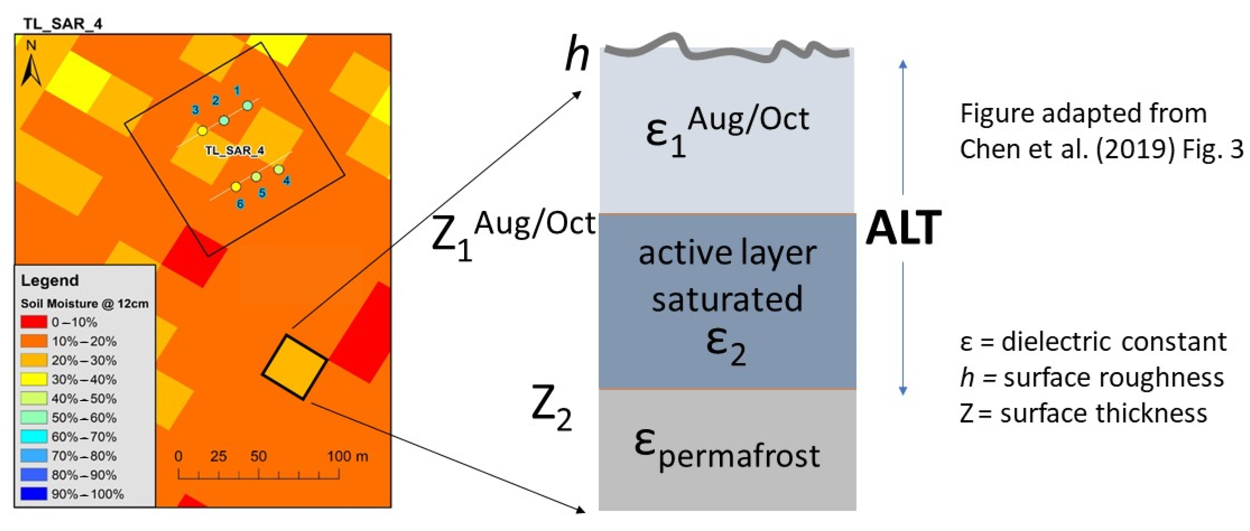
2.2. The Response Feature: SAR-Derived Root-Zone Soil Moisture

The AirMOSS instrument provides high-resolution observations of root-zone soil moisture (RZSM) using polarimetric P-band (420–440 MHz) backscatter [43]. The design for the AirMOSS instrument is leveraged from the L-band Uninhabited Aerial Vehicle Synthetic Aperture Radar (UAVSAR), which has been in use since 2007 [44,45]. The AirMOSS instrument can penetrate deeper into the root zone of vegetation due to its longer wavelength. With a spatial resolution of 10 m and a penetration depth of 0.4–0.6 m, it is ideal for creating regional root-zone soil moisture products at 30 m resolutions [41,46]. In permafrost regions, the AirMOSS instrument has acquired data during four phases of permafrost thaw: thaw onset (late May to early June), maximum thaw (late August), partially frozen (early October), and fully frozen (early-mid April).
To derive soil moisture from the polarimetric radar backscatter collected by AirMOSS, Chen et al. (2019) used a three-layer dielectric forward inversion model. The major challenge presented by this retrieval is the simultaneous estimation of multiple geophysical parameters, which are often ambiguous in the radar backscatter. A time-series approach resolves this ambiguity by assuming vegetation, surface roughness, and the change in thaw depth do not vary significantly between observations. For the Seward Peninsula dataset, the AirMOSS instrument was flown near the maximum thaw (17 August 2017) and partially frozen (10 October 2017) time periods. Between late August and early October, it is assumed that the upward freezing of the active layer is minimal because heat input to the subsurface is limited, therefore it can be approximated to represent the maximum active layer depth [47]. Surface air temperatures and soil temperatures at 5 cm below the ground surface at a meteorological station within the ROI (Teller Site MM27 as shown in Figure 1) indicate that the onset of freezing occurs after 15 October 2017 and should not interfere with the retrieval of the root-zone soil moisture product. Additionally, snow does not present a major concern because the dielectric constant of snow is similar to that of frozen soils and is lumped into the retrieval of the surface layer dielectric (ε1) [41]. Snow at the meteorological stations Teller Site MM27 indicate that snow cover on 15 October 2017 (earliest measurement) is <2 cm.
The Chen et al. (2019) product [48] models the dielectric properties of three soil layers: the unsaturated surface active layer, the saturated active layer, and the underlying permafrost (Figure 2). Using empirical calibrations based on Alaskan soils, we convert soil dielectric constants into volumetric water contents (VWC) at three depths (6 cm, 12 cm, and 20 cm) that can be compared directly against in situ observations of the VWC at the same depths using time-domain reflectometry [49]. To facilitate comparison, SAR-derived dielectric constants were converted to VWC using Equations (1) and (2) which converts the real dielectric constant to τ , the time period of returned signal for the in situ TDR devices.
τ = τ 0 + 2 L c L R e { ϵ r } R e { ϵ r } ϵ r = c 0 2 L ( τ τ 0 )
where c 0 is the speed of light in free space, ϵ R is the relative permittivity/dielectric constant ( ϵ r = ϵ r + i ϵ r ), τ is the time period of the returned signal, τ 0 is the time delay due to internal circuits, and L is the length of the waveguide (probe rods). In-situ measurements for 6 cm, 12 cm and 20 cm soil depths were taken with different Hydrosense II probe (CS620) rod lengths (6 cm and 12 cm w/CS659, 20 cm w/CS658), which requires two quadratic calibration equations that are used in a weighted average to get the SAR-derived VWC.
θ = A τ 2 + B τ + C  
where θ is the volumetric water content, τ is the period in microseconds, and A, B and C are derived from calibration data based on gravimetric moisture observations from soils collected in the Northwest Territories, Canada [49]. Coefficients used can be found in the Appendix A in Table A1.

2.3. Predictor Features

Models of soil moisture commonly incorporate three complex and overlapping environmental controls: local topography, soil conditions, and vegetation cover [10,11,12,13]. We exclude soil conditions due to a lack of comprehensive soil information on the Seward Peninsula. Instead, we focus on a mixture of proven and easily accessible topographic, vegetation, and meteorological features to predict the SAR-derived root-zone soil moisture. By doing so, this method can be applied to a broader array of environments and regions to increase its application external to this work.

2.3.1. Topographic Features

Topographic features were derived from an Interferometric Synthetic Aperture Radar (IfSAR) Digital Terrain Model (DTM) of Alaska with a 5 m spatial resolution (data available from http://ifsar.gina.alaska.edu/ accessed on 29 October 2021) The DTM differs from its accompanying data product, a Digital Surface Model (DSM), by the removal of vegetation and man-made feaures resulting in bare earth elevations. Using ArcGIS 10.8, we created rasters for elevation, slope, curvature, and topographic position index (TPI). Additionally, we calculate the SAGA (System for Automated Geoscientific Analyses) wetness index (SWI) using QGIS. Each of these indices is described below. The reason for using both programs is because the mapping of points to raster values is more efficient in QGIS and the SAGA tools were easier to implement. However, the same results can be achieved by both.
In Arctic regions, spatially extensive soil moisture measurements are challenging and expensive to obtain, thus terrain-based surrogates, such as wetness indices are commonly used. Thus, TPI and SWI reflect topographic controls on the spatial variation of soil moisture, and do not consider precipitation events, vegetation, or soil conditions [50]. These indices generally represent spatial distributions of soil moisture based on the flow of water over the landscape and have been shown to work best for predicting soil moisture deeper (>0.4 m) in the land surface [50,51,52].
TPI measures the relative topographic position of a central pixel as the difference between the elevation of the central pixel and the mean elevation of the neighboring pixels [53]. Positive and negative values correspond to ridges and valleys, respectively, while zero values correspond generally to flat areas. TPI has been used to classify morphological landscapes for environmental analysis [54,55].
The SAGA Wetness Index (SWI) is a modification of the commonly used topographic wetness index (TWI) [56], adapted to detect small changes in elevation in regions with low relief by using an iterative modification of the specific catchment area [57]. SWI is applied as a proxy for soil water accumulation (Equation (3)) [58,59].
S C A M = S C A m a x   ( 1 15 ) β e x p   ( 15 β )     for   S C A < S C A m a x ( 1 15 ) β e x p ( 15 β ) S W I = ln ( S C A M tan β )
where β is the slope angle, SCA is the specific catchment area, S C A M is the modified specific catchment area, and t a n   ( β )   is the local slope [60].

2.3.2. Vegetation Features

Using the Google Earth Engine (GEE) Code Editor and the GEE Data Catalog, we downloaded Landsat 8 Collection 2 (Analysis Ready Data, ARD) imagery for the ROI to estimate vegetation features [61]. Using a cloud threshold of 80%, we took the median of images collected within one week (before/after) of the flights for years 2016, 2017, and 2018. Clouds were then masked using the FMask v3.3.1 algorithm [62] as well as the simpleCloudScore function (<20% cloud probability accepted) in GEE. We took the median pixel value from images that covered more than 50% of the region of interest to get a complete cloud-free mosaic
We calculated three vegetation indices using the Landsat mosaic including the Normalized Difference Vegetation Index (NDVI), the Landsat Enhanced Vegetation Index (EVI), and the Tasseled Cap Greenness (TCG) index [63,64]. The NDVI is among the most used Landsat indices because it quantifies the greenness of vegetation. NDVI is calculated from near-infrared light and visible wavelengths and ranges from −1 to 1, with values closer to one representing the most dense and green leaves. NDVI has been used to assess vegetative change in above-ground biomass and quality across landscape scales [65,66,67,68,69,70]. Landsat Enhanced Vegetation Index (EVI) reduces atmospheric influences while being more sensitive in regions with high biomass by decoupling the atmospheric influences from the canopy background signal [71]. TCG incorporates more bands than NDVI and has been shown to better approximate vegetation biomass [72]. While random forest models are well equipped to handle correlated features, we included only the single highest scoring of the three vegetation indices in each final model [73].

2.3.3. Meteorological Features

Meteorological variables are key to soil moisture distributions on a landscape, however fine-scale measurements over vast and remote areas of Alaska are sparse. Wind and radiation indices based on topography (slope/aspect) help to account for these important processes in our model and represent peak snow depth and the sum of radiation for each pixel.
Solar radiation is distributed unevenly on north and south-facing slopes, creating soil temperature variations that impact evapotranspiration and hence, soil moisture conditions [10,74,75]. Therefore, radiation was included as a predictor feature through the use of the Areal Solar Radiation (ASR) tool in ArcGIS 10.8, which calculates the sum solar insolation (WH/m2) for a given digital terrain model, period of time, and latitude. In this case, summer ASR was calculated between 1 May 2017 and 1 October 2017 to capture the entirety of the snow-free season.
Wind is also a critical driver of evapotranspiration patterns, however local wind speed and direction are challenging to predict over large areas with sparse data. Wind-borne transport of snow occurs at speeds above 6 m/s where it is eroded from windward slopes and deposited on leeward slopes [76]. A wind factor from −1 to 1 is used to show the change in angle from a windward to a leeward slope, where leeward slopes are negative [77]. In this case, the predominant direction of the wind was from the East (90 deg), we use Equation (4). More detail can be found in Appendix A.1.
W f ( A ) = s i n ( A )
where W f is the wind factor and A is the aspect of the slope in radians.

2.4. Modelling

A random forest model was chosen to account for the nonlinear relationships between predictor features and the SAR-derived root-zone soil moisture product from Chen et al., 2019. Random forests are based on decision trees composed of yes/no binary choices to predict a dependent or response variable. Each tree considers a different combination of questions that generate a “vote” for the class (classification) or mean prediction (regression), and the one with the most votes is used as the final prediction. By using an ensemble with many trees, random forest models mitigate the errors made by individual trees to make robust predictions.
The random forest approach is useful because it handles both categorical and continuous variables, is efficient on a large database, is less influenced by outliers, implicitly handles collinearity of variables, and can be applied to determine feature importance [78]. Disadvantages of random forest models are that it can be hard to separate the impact of individual variables as they are rooted deeply in various trees. Random forest models were constructed using the RandomForestRegressor within the Python scikit-learn package. Scoring of models is assessed using the coefficient of determination (R2) because it is normalized between 0 and 1, making it more easily interpretable as a best fit statistic.
Feature importance in random forests are commonly calculated in two ways: impurity feature importance and permutation feature importance. Impurity importance, also known as Mean Decrease in Impurity (MDI), is proportional to the total number of splits that each feature divides across all trees in the random forest, where features with more splits are more important [78]. MDI feature importance is computationally cheap but can be biased towards features with more possible split points, thus it can suffer from overfitting. Permutation importance, also known as Mean Decrease in Accuracy (MDA), is based on the decrease in model performance when a single feature is randomly shuffled, more important features result in larger decreases in performance when permuted [78]. In selecting scales and features, we opted for MDA because it tests the impact of the variables itself rather than using a statistical analysis of the tree structure, which may be influenced by overfitting.
Cross-validation (CV) was performed at every step of the fitting procedure to mitigate overfitting and ensure consistent results. We use a cross-validation procedure in which a random 80% of the dataset was selected for training and 20% withheld for testing during each model run. This is instituted using sklearn’s ShuffleSplit function.
The fitting procedure consists of an initial resolution selection, hyperparameter tuning, recursive feature elimination, collinearity analysis (Pearson’s Correlation, Variance Inflation Factor, VIF), and the final resolution selection. A diagram of this procedure is shown in Figure 3.

2.4.1. Selecting Resolutions

The initial dataset contains all ten features at six separate resolutions (30 m, 60 m, 90 m, 120 m, 180 m, 240 m). All features were normalized to a mean value of 0 and a standard deviation of 1. Initial resolutions were selected from the highest scoring resolution for each of the ten features based on the MDA score with a cross-validation of 30. After tuning hyperparameters, recursive feature elimination, and eliminating features based on collinearity, the final feature resolutions were identified using a grid search with a cross-validation of 5.

2.4.2. Tuning Model Hyperparameters

Tuning a random forest involves changing parameters that define the shape of individual decision trees. There are numerous hyperparameters that can be used to create an efficient and accurate random forest model. These parameters include: the total number of trees (ntrees), the maximum depth of each tree (max_depth), the minimum number of samples required to split an internal node (min_samples_split), the minimum number of samples required to be at a leaf node (min_samples_leaf), the number of features to consider when looking for the best split (max_features), and whether bootstrapping is used. To find the best hyperparameters, we perform a grid search over ranges of values for each parameter. In total, we fit 118 different configurations with a cross-validation of 5.
When working with random forest models, the number of trees and the maximum depth of each tree generally required the most tuning. In Figure 4, we show that the maximum depth of each tree (max_depth) has a more dramatic effect than the number of trees (ntrees) in determining the score of the model.
Tuning results for all depths were very similar, so we opted to use the same hyperparameters for all three models. Final hyperparameters are provided in Table A2.

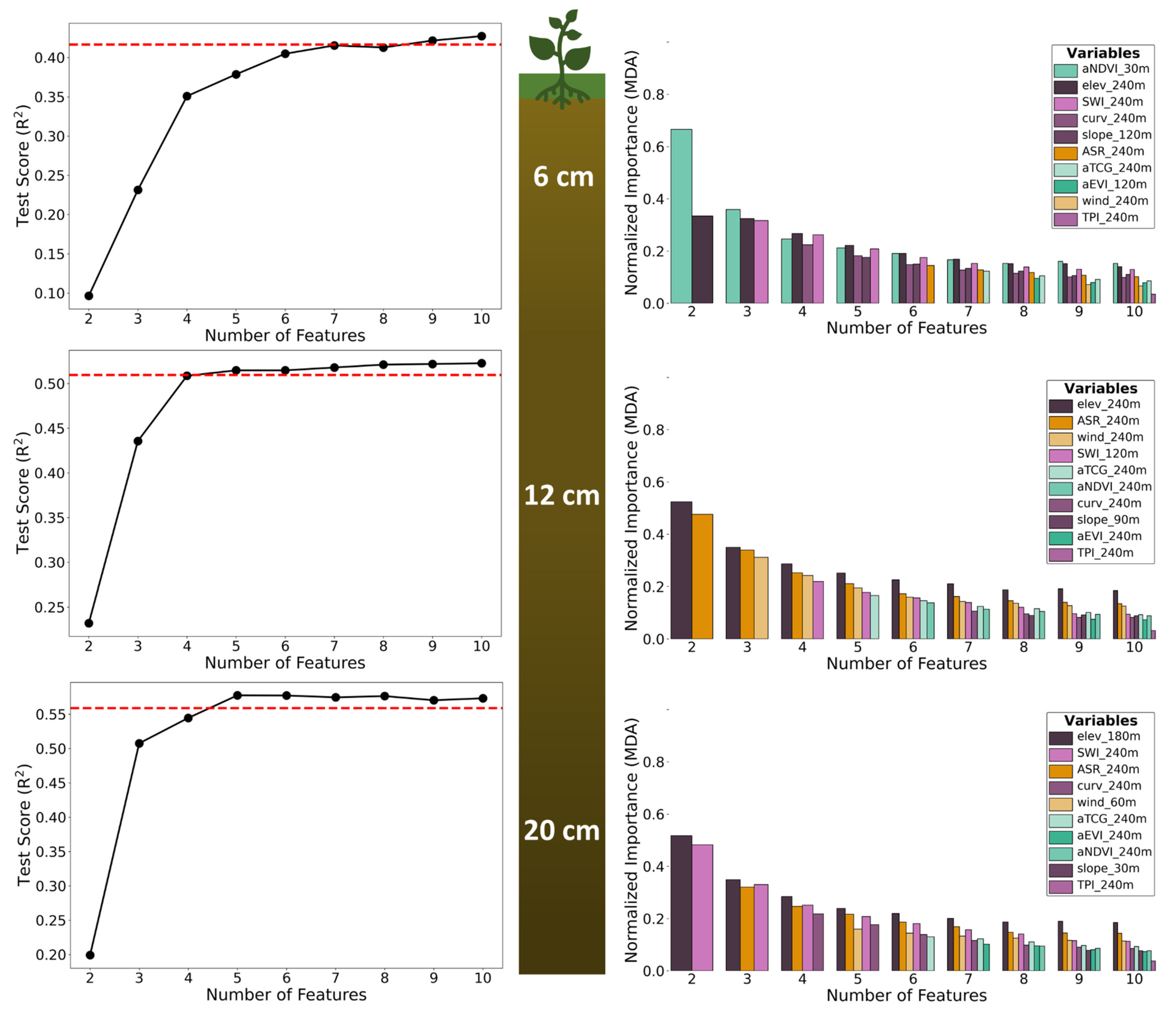
2.4.3. Recursive Feature Elimination

Feature selection was determined using a recursive feature elimination method in which variables are eliminated one at a time based on their MDA importance until there are just two features remaining. Resolutions used in this stage are based on results of the previous step. We use cross-validation of 5 to eliminate the least important feature from ten variables to two. We determine the number of variables for each fit based on where the elimination of a variable results in a loss of >2.5% of the initial coefficient of determination with all ten variables.

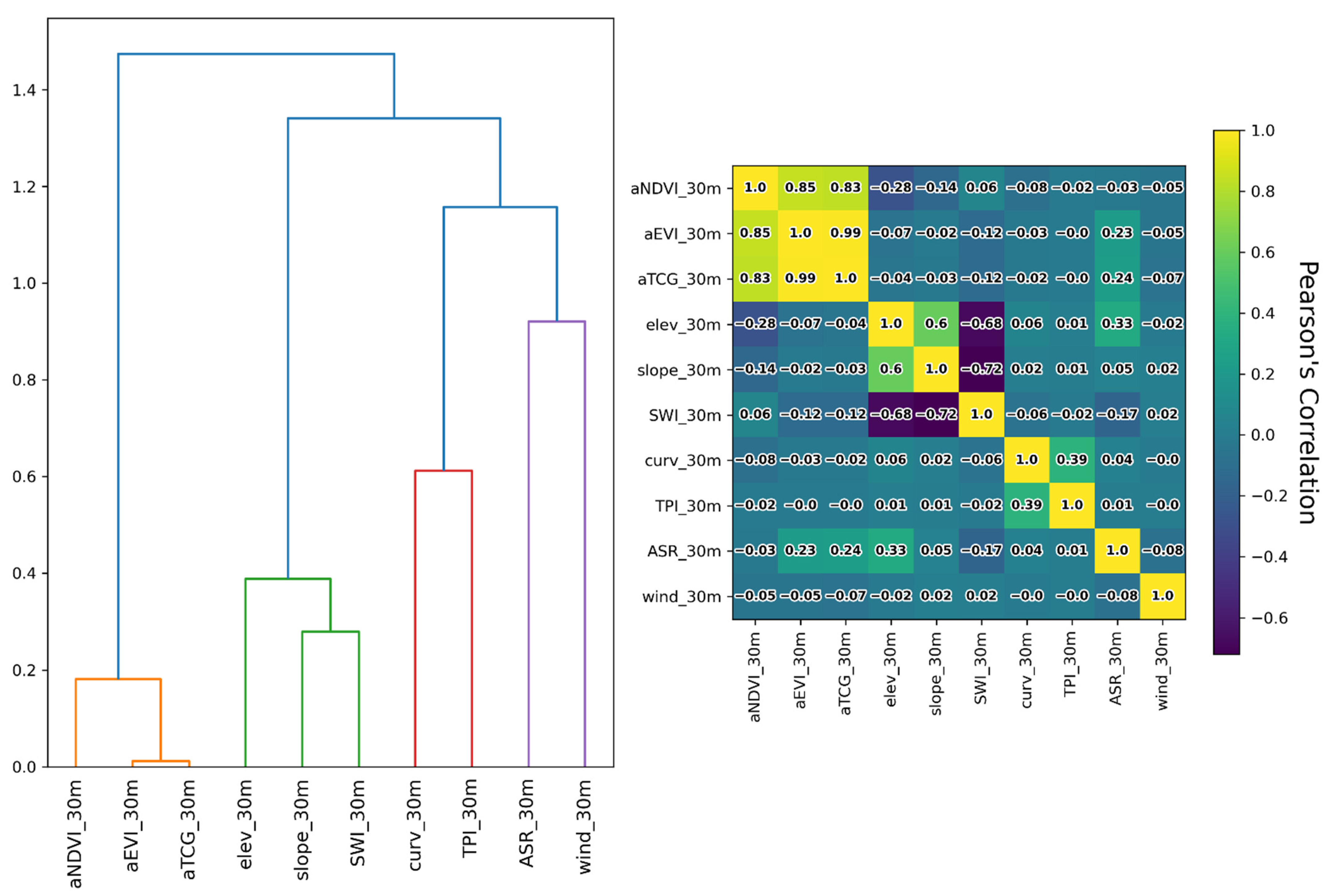
2.4.4. Pairwise Correlation and Multicollinearity

After selecting the best performing feature resolutions, we computed pairwise correlation with Pearson’s coefficients as shown in Figure 5.
Using the Pearson’s correlation matrix as distances, Ward’s method identifies clusters of similar variables. The clustering analysis shown on the left side of Figure 5 identifies four groups of features: the Landsat-8 derived vegetation features, major topography, minor topography, and meteorological factors. The major topographic cluster includes elevation, slope, and SWI. SWI is negatively correlated with slope, which is in turn correlated with elevation (e.g., high elevations are generally mountain peaks that are characterized by steep slopes). The minor topographic cluster includes curvature and TPI which are both useful in identifying ridges and valleys. They show a moderate correlation (0.39 for TPI and curvature) with each other. The final cluster included the meteorological features: wind and ASR. Both features address important meteorological influences on soil moisture through the redistribution of snow and total summer radiation based upon topographic exposure. In addition to testing for pairwise correlation, we assess the presence of multicollinearity in the final models and between all variables using the variance inflation factor (VIF) shown in Figure A2 and Figure A3. All VIF values are well below the accepted threshold of five [80] except for the vegetation features.

3. Results

3.1. AirMOSS P-Band SAR-Derived Soil Moisture Product

The SAR-derived soil moisture product for the ROI contains ~2.3 million observations with a mean VWC and a standard deviation of 0.26 +/−0.07, 0.38 +/−0.11, 0.52 +/−0.10 (%/100) for 6 cm, 12 cm, and 20 cm soil depths, respectively. Additionally, the mean error of the reported 6 cm, 12 cm, and 20 cm VWC values are 0.04, 0.15, and 0.25 (%/100) based on uncertainty associated with the retrieval of the dielectric constant ɛ1 and the depth of the surface layer z1. The minimum VWC value detected by the SAR instrument was 0.08 (%/100) and the maximum was 0.76 (%/100). In all cases, the soil moisture of deep layers is greater than shallow regions because the lower active layer, which lies just above the permafrost layer, is assumed to be saturated.
The soil moisture predictions based on random forest models compared to the SAR-derived soil moisture for 6 cm, 12 cm, and 20 cm depths are shown in Figure 6. In each case, the predicted soil moisture distribution is narrower than the SAR-derived values but has a similar mean value. The predicted distributions are more normally distributed whereas the SAR-derived values for deeper soils (12 cm, 20 cm) are broader.

3.2. Random Forest Modeling

Through several different tests, we determined the optimal features and resolutions used in the final models. Initial training included a fit of all 60 feature/resolution combinations to determine initial resolutions for each feature using shuffled cross-validation of 30. We tuned the hyperparameters including the number of trees and the depth using a grid search approach with 118 combinations and shuffled cross-validation of three (final parameters can be found in Table A2). Next, we performed recursive feature elimination based on elimination of the least important feature from ten variables to two. The number of variables included in the final fit for each depth is determined as the point at which loss to the model exceeds 2.5% of the coefficient of determination of the fit with all ten features (Figure 7). Based on these criteria, the 6 cm fit should have seven variables while the 12 cm and 20 cm fits should each have five variables.
After identifying the number of features, we look at feature correlations and multicollinearity. In the 6 cm fit, we eliminated the slope feature as it was less important than SWI. The largest pairwise correlation coefficient between features in the final models are well below the accepted threshold of 0.7, with the exception of slope, elevation, and SWI. SWI and slope have the highest correlation, therefore we only include the best performing in the final model. While elevation and SWI are negatively correlated (−0.72), we chose to include them because the variance inflation factors remain low (<5) [80], random forests have been proven to deal well with collinearity between predictor features [81], and models performed significantly (>2.5%) better when including both SWI and elevation in the same model.
The final step was to determine the final feature resolutions through a grid search approach with shuffled cross-validation of five. Final model predictions and feature importances (MDA) for 6 cm, 12 cm, and 20 cm VWC are shown in Figure 8.
Training and test scores for each model are given in Table 1. The 6 cm model captured 45% of the variance in VWC and has an RMSE of 5.0% on the test set. The 12 cm model captured 52% of the variance in VWC and has an RMSE of 7.6% on the test set. The 20 cm model captured 58% of the variance in VWC and has an RMSE of 6.6% on the test set.

3.3. Feature Importance

Figure 8 shows the permutation feature for the final models. At the shallowest depth (6 cm), vegetation is the most important feature, but in the deeper models its importance becomes insignificant. Overall, elevation and SWI are the important features for predicting VWC distributions across these regions of the Seward Peninsula. In the 12 cm and 20 cm layers, ASR joins elevation and SWI as the three most important features. TPI did not have a significant effect on any of the final models.

4. Discussion

The fate of permafrost in Earth System Models (ESMs) remains highly uncertain as estimates of permafrost carbon-climate feedbacks vary greatly [82]. Soil moisture in the changing Arctic has important implications for land-atmosphere carbon exchange, vegetation distribution, local hydrology, and the thermal regime of underlying permafrost [4,5,6,10]. Field studies indicate that warming and drying lead to higher soil respiration and laboratory studies indicate that carbon losses increase with increased hydrologic drainage [8,83,84]. In the presence of increased saturation of Arctic soils (due either to projected increases in precipitation or ponding caused by thermokarst), microbial decomposition is likely to emit a higher proportion of methane (CH4) to carbon dioxide (CO2) than in dry environments [85]. These local-scale changes, in turn, will have dramatic influence on the global carbon cycle and contribute to climate change [86]. The inclusion of remotely sensed soil moisture products in ESMs has been shown to improve the estimation of soil temperature for permafrost regions [87]. Further understanding of environmental controls on soil moisture at larger scales is critical to improving future studies and models in regions with discontinuous permafrost.
In the absence of highly localized precipitation data across regional scales, secondary factors like topography, vegetation, and meteorological factors play an important role in the redistribution of water through the environment. Using random forest models, we quantify the contribution of individual features and resolutions across three soil depths in the root-zone (6 cm, 12 cm, and 20 cm) that correspond to typical sampling depths specified by NASA ABoVE in situ measurement protocols (see data availability section for details on in situ sampling procedure).
Regional-scale soil moisture estimates from SAR instruments are an important step in moving from field-based observations to global representations. Our results, based on a regional product over discontinuous permafrost, indicate that vegetation (NDVI) is the most important factor influencing shallow depths (6 cm). However, deeper in the soil column, the influence of vegetation is replaced by topographic and meteorological controls. Thus, as shrubs expand northward in the Arctic, near-surface water availability may decrease as these shrubs use the water for important ecohydrological functions [88]. Changes deeper in the soil column will likely be increasingly influenced by the formation of hydrologic pathways driven by topography as permafrost thaw continues.
Drivers of soil moisture distributions in regions underlain by permafrost are understudied when compared to lower latitude regions. There have been in situ studies of individual drivers of soil moisture in permafrost regions [10,14,15,16], but few studies address how these drivers compare to one another [89]. No other study we are aware of attempts to quantify the role of individual features in soil moisture distributions in regions with discontinuous permafrost using P-band SAR that is capable of covering regions necessary for the validation of ESMs. Our study presents a novel approach to understanding the importance of individual drivers across the root zone of regions with discontinuous permafrost. These findings are critical to improving ESMs and regional datasets used in their validation. Additional studies of the in-situ data associated with the NASA ABoVE campaign would greatly contribute to these findings.

4.1. Decreasing Importance of Vegetation in The Soil Column

As depth in the soil column increases, the importance of vegetation in the model decreases. In these modeling efforts, we use only continuous measures of vegetation: NDVI, EVI, and TCG. Coarse-scale NDVI is the most important variable explaining the variance of soil moisture at 6 cm across the landscape. However, no vegetation features are included in the final 12 cm and 20 cm models. This is reflective of the shallow rooting depth of many Arctic tundra species, where the average rooting depth in tundra environments is just 0.5 +/−0.1 m [90].
In the Arctic, increases in NDVI have been attributed to the expansion of deciduous shrubs [65]. Areas dominated by tall willow and alders, trap snow readily creating both a greater availability of water as well as moisture demand during the growing season [18,90,91,92]. Binning of the interaction between NDVI at 240 m and VWC at 6 cm, shows a peak at an NDVI value of ~0.5 and a local minimum at ~0.8 as shown in Figure A4. High NDVI values are associated with dense patches of alder/willow shrubs [65,88,93,94]. This suggests that alder/willow shrublands deplete the water available in the upper layer of soil by this mid-August observation and therefore are a dominant factor in the final fit for 6 cm. The expansion of alders shrubs is correlated with a deepening of the active layer and increased evapotranspiration, both of which lead to lower soil moisture [95]. This conclusion is corroborated by field observations in the region showing that soil moisture at 15 cm in low-lying alder savannas was much greater than in taller alder shrublands (51.1% vs. 30.4%, p = 0.01, [96]) [97]. It is worth noting that elevation becomes the most important feature in the model for fits at 12 cm and 20 cm. This could be due to a variety of factors including increased precipitation at high elevations [98,99], higher wind speeds leading to an increased redistribution of snow [99,100,101], and the draining of water to lower elevations [102,103].

4.2. Increasing Accuracy of Models at Greater Depths in The Soil Column

As depth in the soil column increased, the performance of our random forest models increased, while requiring fewer predictive features. This may be because subsurface hydrologic pathways are controlled by frost table topography and broad-scale topography [104,105]. This is supported by the resulting importance of elevation, SAGA Wetness Index (SWI), and Curvature at 240 m scale in the 12 cm and 20 cm models. The resolution of the initial SAR-derived soil moisture dataset (30 m) may not be fine enough to identify localized changes in hydrology caused by the development of taliks, which allow hydrologic drainage to sub-permafrost layers. With a finer resolution, the presence and state of permafrost could be inferred through study of soil moisture patterns in discontinuous permafrost regions. Our results demonstrate that controls on soil moisture spatial distribution, in a discontinuous permafrost landscape, differ based on depth in the soil column, with varying importance of factors that also depend on depth. An analysis of controls on in situ soil moisture measurements in this region would bolster this result but is outside the scope of the current work.

4.3. Importance of Winter Snow Accumulation on Soil Moisture

Snow plays a fundamental role in controlling water availability, soil temperature, and moisture, which in turn affects all components of Arctic ecosystems [106,107]. As snow melts in spring and summer, localized regions of deep snow, driven by curvature, wind (slope/aspect), elevation, and microtopography, maintain cold temperatures and increase water availability into the growing season. In a positive feedback loop, this can lead to increased growth of deciduous shrubs that are known to trap snow during wind redistribution [76,108,109]. Fine-scale (10–100 m) snow water equivalent (SWE) distributions at regional scales would improve our understanding of summer soil moisture distribution. However, in its absence, we include a wind factor to account for the redistribution of snow in predicting soil moisture. It is well documented that snow is blown off windward facing slopes and accumulates on leeward slopes [106,110,111]. Wind proved to be a significant variable at all depths, however, it generally was one of the least important in predicting the soil moisture distribution. This could be due to the complicated interaction between the trapping of snow by tall shrubs and their increased water uptake, or the capacity of our simple wind index to capture wind effects.

4.4. Mitigating Collinearity and Overfitting in Random Forest Modelling

De-correlation effects from bootstrapping make predictions from the random forest robust to collinearity between features [81]. This is very important because collinearity is inherent to topographic, vegetation, and meteorological features that are often driven by their interaction. We test for both collinearity and multicollinearity before finalizing the model results. Thus, we eliminate highly correlated features in the final model [81]. We also assess for multicollinearity using the VIF between predictor features.
We reduce overfitting throughout the fitting process by cross-validating results and tuning hyperparameters that dictate the number and depth of trees. Random forest models leveled out with a maximum depth of 30 and 50 trees, but parameters min_samples_leaf and min_samples_split had less dramatic influences on the final scores of each model.
Throughout the fitting process, the importance of selected features are highly stable because of the very large number of observations in the P-Band SAR product. For each stage of testing, the dataset was separated into training (80%) and testing (20%) sets to ensure that we have an adequate sample for both. With nearly 2.4 million pixels, training sets of 80% can represent many different environments. In addition, to separate training and testing data, we also used bootstrapping for each model and tested the Out Of Bag (OOB) error and found that values were comparable with the cross-validated test scores (R2).
While the final R2 values could be considered low when compared with more constrained problems, here we purposefully do not include the key input to soil moisture, precipitation, to better constrain secondary features. These secondary features, topography, vegetation, and derived meteorological indices, are responsible for the redistribution of water throughout the ecosystem. By fitting for secondary features, we help global scale models identify critical variables for predicting future soil moisture distributions and in turn greenhouse gas emissions in regions underlain by permafrost. However, the p-values associated with our random forest model are very low because of the high number of observations and give us confidence in the significance of these results.

4.5. Other Key Controls on Soil Moisture

To increase the accuracy of our soil moisture predictions we need to account for fine-scale microtopography and improved soil texture data in the region. Near-surface soil moisture has been shown to be influenced by local microtopography that allows for the accumulation of precipitation in Alaskan permafrost environments [112]. Due to the scale of the SAR-derived soil moisture product, the direct impact of fine-scale microtopography is unable to be confirmed in our modelling efforts. Heterogeneity of soil moisture over short scales (<10 m) are below the grid size for many modern remote sensing techniques as well as modelling efforts. With improved resolution, future SAR missions may become capable of monitoring fine-scale soil moisture in hydrologically complex regions such as the sites described in this work.
In Arctic regions, soil texture data is limited and sparsely distributed resulting in coarse spatial distributions of soil properties that would not aid in the derivation of the soil dielectric constant from radar backscatter. Physical properties of soil including grain size, bulk density, temperature, and organic matter content dictate the water storage capacity [10,28,113], therefore there is a great need for improved soil classifications across Western Alaska. The derivation of soil moisture from P-Band SAR backscatter employed in Chen et al. 2019, uses a constant ratio of the imaginary to the real part of the soil dielectric constant (ϵ’’/e’) of 0.15. For the purpose of this study, we were advised to use the general soil parameters for calibrating our in-situ Time Domain Reflectometry (TDR) soil moisture probes (HydroSense CS620), thus the SAR-Derived soil moisture product was also calibrated using the general soil calibration parameters [49]. These general calibration parameters seem to overestimate the capacity of these soils to store water as evidenced by the maximum volumetric water content recording of 0.76 (%/100).

4.6. Inherent Limitations of The SAR-Derived Soil Moisture Product

All of this work is based on training a P-Band SAR product that has inherent assumptions. The product as described in Chen et al. (2019), assumes a two-layer (surface and saturated layers) dielectric model for the active layer that approximates the actual soil dielectric profile that in reality could be influenced by soil organic matter and soil texture. As previously stated, we used the general calibration coefficients based on Alaskan soils [49]. The P-Band product only covers areas that are bare soil or lightly vegetated because the forward scattering model used does not apply to forested pixels.
The dielectric model also assumes that certain characteristics remain constant between August and October observations, including the surface roughness and the depth of the active layer. The freezing of the active layer occurs from the top down as well as from the bottom up. Freeze-up of the active layer occurs gradually while the ground surface temperature is below 2 °C but above 0 °C [114,115]. At a meteorologic station situated within the ROI surface (1.5 m) air temperatures and soil temperatures at a depth of 5 cm do not go below 2 °C consistently until 15 October 2017. Thus we assume that freezing from the top and from the bottom of the active layer does not begin until after the 10 October 2017 data collection date.
While Chen et al. (2019), provides ground-based validation for the derived active layer thickness using measurements from Circumpolar Active Layer Monitoring sites, they do not address validation of the root-zone soil moisture within the paper. However, researchers have validated the retrieval of root-zone soil moisture from P-band SAR in sub-arctic environments [116]. In-situ measurements taken coincident with SAR flights at three NGEE-Arctic field sites within the ROI are presently insufficient to validate this particular swath and further effort to provide in-depth validation measures is outside the scope of this study.
The dielectric model assumes that the lower layer of the active layer is saturated as it lies just above the nearly impermeable permafrost layer. However, due to the presence of taliks, and other subsurface permafrost drainage features, lower layers of permafrost may not always be wetter than the surface layers. This assumption in the model may apply better in regions of continuous permafrost than in more complex regions such as the Seward Peninsula. Talik features may be present at sub-pixel scales, but their impact on hydrologic drainage could extend beyond the bounds of a single pixel.

5. Conclusions

Root-zone soil moisture is a dominant control on the surface energy balance, carbon fluxes, and vegetation distribution in permafrost landscapes. However, soil moisture predictions in earth system models which rely heavily on soil moisture to approximate carbon fluxes in permafrost environments, vary greatly between different models [117]. The development of P-Band synthetic aperture radar as a tool for estimating active layer properties, including its thickness and soil moisture, is an opportunity to understand complex interactions between vegetation, soil, and water. Until recently, soil moisture studies in remote regions of Alaska have been limited to either discrete in-situ measurements limited in both time and space, or very coarse surface soil moisture measurements. Regional soil moisture products (such as Chen et al. 2019) are bridging the gap by estimating soil moisture within the root zone at finer (10–100 m) resolutions for permafrost regions. In this work, we used random forest models trained on common topographic, vegetation, and meteorologically based features to predict soil moisture distributions based on training datasets with these SAR-derived observations. By doing so, we hope to improve the accuracy with which ESMs approximate soil moisture in regions with discontinuous permafrost.
Results of our work indicate that the primary variables impacting the distribution of soil moisture differ throughout the soil column. At 6 cm, NDVI is the most important variable in determining the soil moisture, however, deeper in the soil column (12 cm and 20 cm) we observe a decay in the importance of vegetation features. Vegetation control on shallow soil moisture is likely due to increased water uptake by willow/alder shrub complexes, leaving these sites drier by the mid-August observation used in this project. At 12 cm and 20 cm soil depths, the most important features are coarse resolution topography and proxies for meteorology (radiation + wind). Additionally, both the 12 and 20 cm depths are easier to predict owing to greater insulation from surface features and processes that increase soil moisture variability, including vegetation and evapotranspiration.

Author Contributions

J.D. designed, implemented, and wrote the manuscript. K.E.B. greatly contributed to the methodology, editing, and conceptualization of the manuscript, while W.R.B. and C.J.W. contributed to the conceptualization of the manuscript and provided edits to the text. All authors have read and agreed to the published version of the manuscript.

Funding

Funding for this research was provided by the Department of Energy Office of Science, Office of Biological and Environmental Research through the Next Generation Ecosystem Experiment (NGEE) Arctic project. Additional funding was provided by the U.S. Geological Survey’s Alaska Climate Adaptation Science Center (Cooperative Agreement G17AC00213).

Data Availability Statement

The P-band SAR dataset can be downloaded from Chen, R.H., A. Tabatabaeenejad, and M. Moghaddam. 2019. aBoVE: Active Layer and Soil Moisture Properties from AirMOSS P-band SAR in Alaska. ORNL DAAC, Oak Ridge, Tennessee, USA. https://doi.org/10.3334/ORNLDAAC/1657 (accessed on 22 October 2021). In situ soil moisture measurements at NGEE Arctic field sites can be downloaded from Wilson C.J., Dann, J., Bolton, W.R., Charsley-Groffman, L., Jafarov, E., Musa, D., Wullschleger, S. 2018. In Situ Soil Moisture and Thaw Depth Measurements Coincident with Airborne SAR Data Collections, Barrow and Seward Peninsulas, Alaska, 2017. Next Generation Ecosystem Experiments Arctic Data Collection, Oak Ridge National Laboratory, U.S. Department of Energy, Oak Ridge, Tennessee, USA. https://doi.org/10.5440/1423892 (accessed on 22 October 2021).

Acknowledgments

We would like to acknowledge the guidance of Richard Chen with respect to using his data product and additionally to Mahta Moghaddam for making the collection of this dataset possible. We gratefully acknowledge Mary’s Igloo, Sitnasuak, and Council Native Corporation guidance and for allowing us to conduct our research on their traditional lands. We would also like to acknowledge Rawser Spicer for his advice on random forest modeling, and Emma Lathrop, Kyle Dickman, and Xiaoying Jin for assisting with the field data collection. We’d also like to acknowledge our reviewers for their time and expertise that helped this paper come to be.

Conflicts of Interest

The authors declare there are no conflict of interest.

Appendix A

Appendix A.1. Wind Factor Derivation

To derive predominant wind direction, we downloaded weather station data from nearby airports [Teller (PATE), Nome (PAOM), and White Mountain (PAWM)] to obtain the wind directions between 1 October to 1 May for winds in excess of the snow transport threshold (i.e., 6 m/s) [76]. The average wind speed for the stations were: 3.75 m/s (PAOM), 5.1 m/s (PATE), and 4.1 m/s (PAWM). The average wind direction (>6 m/s) were: 80.7 deg (PAOM), 91.2 deg (PATE), and 53.4 deg (PAWM). Based on this we use Equation (4) based on an easterly wind as shown in Figure A1 [77].
Figure A1. Wind factor illustration for an easterly wind were derived similarly to the wind equations found in Dvornikov et al 2015 [55].
Remotesensing 14 04927 g0a1
Figure A2. Variance inflation factors (VIF) for final variables are all well under the accepted threshold of 5 [80].
Remotesensing 14 04927 g0a2
Figure A3. Variance inflation factors for the ten predictor features at their smallest resolutions. The red dashed line shows the accepted threshold of five [80].
Remotesensing 14 04927 g0a3
Figure A4. Boxplots of the VWC at 6 cm binned by the most predictive feature (NDVI @ 240 m) showing a peak at ~0.5 and a local minima at ~0.8.
Remotesensing 14 04927 g0a4
Table A1. Coefficients used to calibrate in situ and SAR-derived volumetric water contents for general Alaskan soil types [49].
GroupProbeProbe DepthABCR2Standard Error
GeneralHydrosense II20 cm7.6931.641−12.3410.88735.773
GeneralHydrosense II12 cm−24.28134.55−110.2450.82947.102
Table A2. Final hyperparameters for the random forest model runs after the grid search selection.
ModelNumber of TreesMax DepthMax SamplesMin_Samples_LeafMin_Samples_SplitBootstrapMax Features
6 cm50300.8110Truesqrt
12 cm50300.8110Truesqrt
20 cm50300.8110Truesqrt

References

  1. Tarnocai, C.; Canadell, J.G.; Schuur, E.A.G.; Kuhry, P.; Mazhitova, G.; Zimov, S. Soil Organic Carbon Pools in the Northern Circumpolar Permafrost Region. Glob. Biogeochem. Cycles 2009, 23, GB2023. [Google Scholar] [CrossRef]
  2. Osborne, E.; Richter-Menge, J.; Jeffries, M. Arctic Report Card 2018; National Park Service: Washington, DC, USA, 2018.
  3. Muller, S.W. Permafrost: Or Permanently Frozen Ground: And Related Engineering Problems; Army Map Service, U.S. Army: Arlington, VA, USA, 1945. [Google Scholar]
  4. Smith, L.C.; Sheng, Y.; MacDonald, G.M.; Hinzman, L.D. Disappearing Arctic Lakes. Science 2005, 308, 1429. [Google Scholar] [CrossRef] [PubMed] [Green Version]
  5. Hinzman, L.D.; Bettez, N.D.; Bolton, W.R.; Chapin, F.S.; Dyurgerov, M.B.; Fastie, C.L.; Griffith, B.; Hollister, R.D.; Hope, A.; Huntington, H.P.; et al. Evidence and Implications of Recent Climate Change in Northern Alaska and Other Arctic Regions. Clim. Chang. 2005, 72, 251–298. [Google Scholar] [CrossRef]
  6. Keller, K.; Blum, J.D.; Kling, G.W. Stream Geochemistry as an Indicator of Increasing Permafrost Thaw Depth in an Arctic Watershed. Chem. Geol. 2010, 273, 76–81. [Google Scholar] [CrossRef]
  7. Liljedahl, A.K.; Hinzman, L.D.; Harazono, Y.; Zona, D.; Tweedie, C.E.; Hollister, R.D.; Engstrom, R.; Oechel, W.C. Nonlinear Controls on Evapotranspiration in Arctic Coastal Wetlands. Biogeosciences 2011, 8, 3375–3389. [Google Scholar] [CrossRef] [Green Version]
  8. Oberbauer, S.F.; Tenhunen, J.D.; Reynolds, J.F. Environmental Effects on CO2 Efflux from Water Track and Tussock Tundra in Arctic Alaska, USA. Arct. Alp. Res. 1991, 23, 162–169. [Google Scholar] [CrossRef]
  9. Schuur, E.A.G.; McGuire, A.D.; Schädel, C.; Grosse, G.; Harden, J.W.; Hayes, D.J.; Hugelius, G.; Koven, C.D.; Kuhry, P.; Lawrence, D.M.; et al. Climate Change and the Permafrost Carbon Feedback. Nature 2015, 520, 171–179. [Google Scholar] [CrossRef] [PubMed]
  10. Isard, S.A. Factors Influencing Soil Moisture and Plant Community Distribution on Niwot Ridge, Front Range, Colorado, USA. Arct. Alp. Res. 1986, 18, 83. [Google Scholar] [CrossRef]
  11. Takahashi, K. Seasonal Changes in Soil Temperature on an Upper Windy Ridge and Lower Leeward Slope in Pinus Pumila Scrub on Mt. Shogigashira, Central Japan. Polar Biosci. 2005, 18, 82–89. [Google Scholar]
  12. Bertoldi, G.; Notarnicola, C.; Leitinger, G.; Endrizzi, S.; Zebisch, M.; Della Chiesa, S.; Tappeiner, U. Topographical and Ecohydrological Controls on Land Surface Temperature in an Alpine Catchment. Ecohydrol. Ecosyst. Land Water Process Interact. Ecohydrogeomorphol. 2010, 3, 189–204. [Google Scholar] [CrossRef]
  13. Scherrer, D.; Körner, C. Topographically Controlled Thermal-habitat Differentiation Buffers Alpine Plant Diversity against Climate Warming. J. Biogeogr. 2011, 38, 406–416. [Google Scholar] [CrossRef]
  14. Aalto, J.; le Roux, P.C.; Luoto, M. Vegetation Mediates Soil Temperature and Moisture in Arctic-Alpine Environments. Arct. Antarct. Alp. Res. 2013, 45, 429–439. [Google Scholar] [CrossRef] [Green Version]
  15. Ayres, E.; Nkem, J.N.; Wall, D.H.; Adams, B.J.; Barrett, J.E.; Simmons, B.L.; Virginia, R.A.; Fountain, A.G. Experimentally Increased Snow Accumulation Alters Soil Moisture and Animal Community Structure in a Polar Desert. Polar Biol. 2010, 33, 897–907. [Google Scholar] [CrossRef]
  16. Kemppinen, J. Soil Moisture and Its Importance for Tundra Plants; Helsingin Yliopisto: Helsinki, Finland, 2020. [Google Scholar]
  17. Yoshikawa, K.; Hinzman, L.D. Shrinking Thermokarst Ponds and Groundwater Dynamics in Discontinuous Permafrost near Council, Alaska. Permafr. Periglac. Process. 2003, 14, 151–160. [Google Scholar] [CrossRef]
  18. Jafarov, E.E.; Coon, E.T.; Harp, D.R.; Wilson, C.J.; Painter, S.L.; Atchley, A.L.; Romanovsky, V.E. Modeling the Role of Preferential Snow Accumulation in through Talik Development and Hillslope Groundwater Flow in a Transitional Permafrost Landscape. Environ. Res. Lett. 2018, 13, 105006. [Google Scholar] [CrossRef]
  19. Petropoulos, G. Remote Sensing of Energy Fluxes and Soil Moisture Content; Taylor & Francis Group: Baton Rouge, LA, USA, 2013; ISBN 978-1-4665-0579-7. [Google Scholar]
  20. Ahlmer, A.-K.; Cavalli, M.; Hansson, K.; Koutsouris, A.J.; Crema, S.; Kalantari, Z. Soil Moisture Remote-Sensing Applications for Identification of Flood-Prone Areas along Transport Infrastructure. Environ. Earth Sci. 2018, 77, 533. [Google Scholar] [CrossRef] [Green Version]
  21. Crow, W.T.; Milak, S.; Moghaddam, M.; Tabatabaeenejad, A.; Jaruwatanadilok, S.; Yu, X.; Shi, Y.; Reichle, R.H.; Hagimoto, Y.; Cuenca, R.H. Spatial and Temporal Variability of Root-Zone Soil Moisture Acquired From Hydrologic Modeling and AirMOSS P-Band Radar. IEEE J. Sel. Top. Appl. Earth Obs. Remote Sens. 2018, 11, 4578–4590. [Google Scholar] [CrossRef]
  22. Hallikainen, M.T.; Ulaby, F.T.; Dobson, M.C.; El-rayes, M.A.; Wu, L. Microwave Dielectric Behavior of Wet Soil-Part 1: Empirical Models and Experimental Observations. IEEE Trans. Geosci. Remote Sens. 1985, GE-23, 25–34. [Google Scholar] [CrossRef]
  23. Dobson, M.C.; Ulaby, F.T.; Hallikainen, M.T.; El-rayes, M.A. Microwave Dielectric Behavior of Wet Soil-Part II: Dielectric Mixing Models. IEEE Trans. Geosci. Remote Sens. 1985, GE-23, 35–46. [Google Scholar] [CrossRef]
  24. Mironov, V.L.; Dobson, M.C.; Kaupp, V.H.; Komarov, S.A.; Kleshchenko, V.N. Generalized Refractive Mixing Dielectric Model for Moist Soils. IEEE Trans. Geosci. Remote Sens. 2004, 42, 773–785. [Google Scholar] [CrossRef]
  25. Ulaby, F.T.; Siquera, P.; Nashashibi, A.; Sarabandi, K. Semi-Empirical Model for Radar Backscatter from Snow at 35 and 95 GHz. IEEE Trans. Geosci. Remote Sens. 1996, 34, 1059–1065. [Google Scholar] [CrossRef]
  26. Fung, A.K.; Bredow, J.W.; Gogineni, P. An Investigation of Scattering Mechanisms from Snow Covered Ice. In Proceedings of the 1995 International Geoscience and Remote Sensing Symposium, IGARSS ’95. Quantitative Remote Sensing for Science and Applications, Firenze, Italy, 10–14 July 1995; Volume 1, pp. 407–409. [Google Scholar]
  27. Peplinski, N.R.; Ulaby, F.T.; Dobson, M.C. Dielectric Properties of Soils in the 0.3-1.3-GHz Range. IEEE Trans. Geosci. Remote Sens. 1995, 33, 803–807. [Google Scholar] [CrossRef]
  28. Mironov, V.L.; De Roo, R.D.; Savin, I.V. Temperature-Dependable Microwave Dielectric Model for an Arctic Soil. IEEE Trans. Geosci. Remote Sens. 2010, 48, 2544–2556. [Google Scholar] [CrossRef]
  29. Oh, Y.; Sarabandi, K.; Ulaby, F.T. An Empirical Model and an Inversion Technique for Radar Scattering from Bare Soil Surfaces. IEEE Trans. Geosci. Remote Sens. 1992, 30, 370–381. [Google Scholar] [CrossRef]
  30. Taconet, O.; Vidal-Madjar, D.; Emblanch, C.; Normand, M. Taking into Account Vegetation Effects to Estimate Soil Moisture from C-Band Radar Measurements. Remote Sens. Environ. 1996, 56, 52–56. [Google Scholar] [CrossRef]
  31. Quesney, A.; Le Hégarat-Mascle, S.; Taconet, O.; Vidal-Madjar, D.; Wigneron, J.P.; Loumagne, C.; Normand, M. Estimation of Watershed Soil Moisture Index from ERS/SAR Data. Remote Sens. Environ. 2000, 72, 290–303. [Google Scholar] [CrossRef]
  32. Zribi, M.; Dechambre, M. A New Empirical Model to Inverse Soil Moisture and Roughness Using Two Radar Configurations. In Proceedings of the IEEE International Geoscience and Remote Sensing Symposium, Toronto, ON, Canada, 24–28 June 2002; Volume 4, pp. 2223–2225. [Google Scholar]
  33. Le Hegarat-Mascle, S.; Zribi, M.; Alem, F.; Weisse, A.; Loumagne, C. Soil Moisture Estimation from ERS/SAR Data: Toward an Operational Methodology. IEEE Trans. Geosci. Remote Sens. 2002, 40, 2647–2658. [Google Scholar] [CrossRef]
  34. Álvarez-Mozos, J.; Casalí, J.; González-Audícana, M.; Verhoest, N.E.C. Correlation between Ground Measured Soil Moisture and RADARSAT-1 Derived Backscattering Coefficient over an Agricultural Catchment of Navarre (North of Spain). Biosyst. Eng. 2005, 92, 119–133. [Google Scholar] [CrossRef]
  35. Oh, Y.; Sarabandi, K.; Ulaby, F.T. An Inversion Algorithm for Retrieving Soil Moisture and Surface Roughness from Polarimetric Radar Observation. In Proceedings of the IGARSS ’94—1994 IEEE International Geoscience and Remote Sensing Symposium, Pasadena, CA, USA, 8–12 August 1994; Volume 3, pp. 1582–1584. [Google Scholar]
  36. Dubois, P.C.; van Zyl, J.; Engman, T. Measuring Soil Moisture with Active Microwave: Effect of Vegetation. In Proceedings of the 1995 International Geoscience and Remote Sensing Symposium, IGARSS ’95. Quantitative Remote Sensing for Science and Applications, Firenze, Italy, 10–14 July 1995; Volume 1, pp. 495–497. [Google Scholar]
  37. Fung, A.K.; Li, Z.; Chen, K.S. Backscattering from a Randomly Rough Dielectric Surface. IEEE Trans. Geosci. Remote Sens. 1992, 30, 356–369. [Google Scholar] [CrossRef]
  38. Ulaby, F. Radar Measurement of Soil Moisture Content. IEEE Trans. Antennas Propag. 1974, 22, 257–265. [Google Scholar] [CrossRef] [Green Version]
  39. Miller, C.E.; Griffith, P.C.; Goetz, S.J.; Hoy, E.E.; Pinto, N.; McCubbin, I.B.; Thorpe, A.K.; Hofton, M.; Hodkinson, D.; Hansen, C.; et al. An Overview of ABoVE Airborne Campaign Data Acquisitions and Science Opportunities. Environ. Res. Lett. 2019, 14, 080201. [Google Scholar] [CrossRef]
  40. Moghaddam, M.; Tabatabaeenejad, A.; Chen, R.H.; Saatchi, S.S.; Jaruwatanadilok, S.; Burgin, M.; Duan, X.; Truong-Loi, M.L. AirMOSS: L2/3 Volumetric Soil Moisture Profiles Derived from Radar, 2012–2015; ORNL DAAC: Oak Ridge, TN, USA, 2016. [CrossRef]
  41. Chen, R.H.; Tabatabaeenejad, A.; Moghaddam, M. Retrieval of Permafrost Active Layer Properties Using Time-Series P-Band Radar Observations. IEEE Trans. Geosci. Remote Sens. 2019, 57, 6037–6054. [Google Scholar] [CrossRef]
  42. Peel, M.C.; Finlayson, B.L.; McMahon, T.A. Updated World Map of the Köppen-Geiger Climate Classification. Hydrol. Earth Syst. Sci. 2007, 11, 1633–1644. [Google Scholar] [CrossRef] [Green Version]
  43. Chapin, E.; Chau, A.; Chen, J.; Heavey, B.; Hensley, S.; Lou, Y.; Machuzak, R.; Moghaddam, M. AirMOSS: An Airborne P-Band SAR to Measure Root-Zone Soil Moisture. In Proceedings of the 2012 IEEE Radar Conference, Atlanta, GA, USA, 7–11 May 2012; pp. 693–698. [Google Scholar]
  44. Rosen, P.A.; Hensley, S.; Wheeler, K.; Sadowy, G.; Miller, T.; Shaffer, S.; Muellerschoen, R.; Jones, C.; Zebker, H.; Madsen, S. UAVSAR: A New NASA Airborne SAR System for Science and Technology Research. In Proceedings of the 2006 IEEE Conference on Radar, Verona, NY, USA, 24–27 April 2006; p. 8. [Google Scholar]
  45. Hensley, S.; Wheeler, K.; Sadowy, G.; Jones, C.; Shaffer, S.; Zebker, H.; Miller, T.; Heavey, B.; Chuang, E.; Chao, R. The UAVSAR Instrument: Description and First Results. In Proceedings of the 2008 IEEE Radar Conference, Rome, Italy, 26–30 May 2008; pp. 1–6. [Google Scholar]
  46. Tabatabaeenejad, A.; Burgin, M.; Duan, X.; Moghaddam, M. P-Band Radar Retrieval of Subsurface Soil Moisture Profile as a Second-Order Polynomial: First AirMOSS Results. IEEE Trans. Geosci. Remote Sens. 2015, 53, 645–658. [Google Scholar] [CrossRef]
  47. Zona, D.; Gioli, B.; Commane, R.; Lindaas, J.; Wofsy, S.C.; Miller, C.E.; Dinardo, S.J.; Dengel, S.; Sweeney, C.; Karion, A.; et al. Cold Season Emissions Dominate the Arctic Tundra Methane Budget. Proc. Natl. Acad. Sci. USA 2016, 113, 40–45. [Google Scholar] [CrossRef] [Green Version]
  48. Chen, R.H.; Tabatabaeenejad, A.; Moghaddam, M. ABoVE: Active Layer and Soil Moisture Properties from AirMOSS P-Band SAR in Alaska; ORNL DAAC: Oak Ridge, TN, USA, 2019. [CrossRef]
  49. Bourgeau-Chavez, L.L.; Garwood, G.C.; Riordan, K.; Koziol, B.W.; Slawski, J. Development of Calibration Algorithms for Selected Water Content Reflectometry Probes for Burned and Non-Burned Organic Soils of Alaska. Int. J. Wildland Fire 2010, 19, 961. [Google Scholar] [CrossRef]
  50. Western, A.W.; Grayson, R.B.; Blöschl, G. Scaling of Soil Moisture: A Hydrologic Perspective. Annu. Rev. Earth Planet. Sci. 2002, 30, 149–180. [Google Scholar] [CrossRef] [Green Version]
  51. Southee, F.M.; Treitz, P.M.; Scott, N.A. Application of Lidar Terrain Surfaces for Soil Moisture Modeling. Photogramm. Eng. Remote Sens. 2012, 78, 1241–1251. [Google Scholar] [CrossRef]
  52. Murphy, P.N.; Ogilvie, J.; Meng, F.-R.; White, B.; Bhatti, J.S.; Arp, P.A. Modelling and Mapping Topographic Variations in Forest Soils at High Resolution: A Case Study. Ecol. Model. 2011, 222, 2314–2332. [Google Scholar] [CrossRef]
  53. Amatulli, G.; Domisch, S.; Tuanmu, M.-N.; Parmentier, B.; Ranipeta, A.; Malczyk, J.; Jetz, W. A Suite of Global, Cross-Scale Topographic Variables for Environmental and Biodiversity Modeling. Sci. Data 2018, 5, 180040. [Google Scholar] [CrossRef] [Green Version]
  54. Gallant, J.C. Primary Topographic Attributes. In Terrain Analysis-Principles and Application; John Wiley & Sons: Hoboken, NJ, USA, 2000; pp. 51–86. [Google Scholar]
  55. Bennett, K.E.; Miller, G.; Busey, R.; Chen, M.; Lathrop, E.R.; Dann, J.B.; Nutt, M.; Crumley, R.; Dafflon, B.; Kumar, J.; et al. Spatial Patterns of Snow Distribution for Improved Earth System Modelling in the Arctic. Cryosphere 2021. [Google Scholar] [CrossRef]
  56. Beven, K.J.; Kirkby, M.J. A Physically Based, Variable Contributing Area Model of Basin Hydrology/Un Modèle à Base Physique de Zone d’appel Variable de l’hydrologie Du Bassin Versant. Hydrol. Sci. J. 1979, 24, 43–69. [Google Scholar] [CrossRef] [Green Version]
  57. Böhner, J.; Koethe, R.; Conrad, O.; Gross, J.; Ringeler, A.; Selige, T. Soil Regionalisation by Means of Terrain Analysis and Process Parameterisation. Soil Classif. 2001, 7, 213. [Google Scholar]
  58. Böhner, J.; McCloy, K.R. SAGA-Analysis and Modelling Applications. In Collection Göttinger Geographische Abhandlungen; Goltze: Göttingen, Germany, 2006; Volume 115, 130p. [Google Scholar]
  59. Böhner, J.; Selige, T. Spatial Prediction of Soil Attributes Using Terrain Analysis and Climate Regionalisation. In SAGA-Analyses and Modelling Applications; Goltze: Göttingen, Germany, 2006. [Google Scholar]
  60. Zevenbergen, L.W.; Thorne, C.R. Quantitative Analysis of Land Surface Topography. Earth Surf. Process. Landf. 1987, 12, 47–56. [Google Scholar] [CrossRef]
  61. Dwyer, J.L.; Roy, D.P.; Sauer, B.; Jenkerson, C.B.; Zhang, H.K.; Lymburner, L. Analysis Ready Data: Enabling Analysis of the Landsat Archive. Remote Sens. 2018, 10, 1363. [Google Scholar] [CrossRef]
  62. Foga, S.; Scaramuzza, P.L.; Guo, S.; Zhu, Z.; Dilley, R.D.; Beckmann, T.; Schmidt, G.L.; Dwyer, J.L.; Joseph Hughes, M.; Laue, B. Cloud Detection Algorithm Comparison and Validation for Operational Landsat Data Products. Remote Sens. Environ. 2017, 194, 379–390. [Google Scholar] [CrossRef] [Green Version]
  63. Crist, E.P. A TM Tasseled Cap Equivalent Transformation for Reflectance Factor Data. Remote Sens. Environ. 1985, 17, 301–306. [Google Scholar] [CrossRef]
  64. Vermote, E.; Justice, C.; Claverie, M.; Franch, B. Preliminary Analysis of the Performance of the Landsat 8/OLI Land Surface Reflectance Product. Remote Sens. Environ. 2016, 185, 46–56. [Google Scholar] [CrossRef]
  65. Jia, G.J.; Epstein, H.E.; Walker, D.A. Greening of Arctic Alaska, 1981–2001. Geophys. Res. Lett. 2003, 30, 2067. [Google Scholar] [CrossRef]
  66. Myneni, R.B.; Keeling, C.D.; Tucker, C.J.; Asrar, G.; Nemani, R.R. Increased Plant Growth in the Northern High Latitudes from 1981 to 1991. Nature 1997, 386, 698–702. [Google Scholar] [CrossRef]
  67. Stow, D.A.; Hope, A.; McGuire, D.; Verbyla, D.; Gamon, J.; Huemmrich, F.; Houston, S.; Racine, C.; Sturm, M.; Tape, K. Remote Sensing of Vegetation and Land-Cover Change in Arctic Tundra Ecosystems. Remote Sens. Environ. 2004, 89, 281–308. [Google Scholar] [CrossRef] [Green Version]
  68. Goetz, S.J.; Bunn, A.G.; Fiske, G.J.; Houghton, R.A. Satellite-Observed Photosynthetic Trends across Boreal North America Associated with Climate and Fire Disturbance. Proc. Natl. Acad. Sci. USA 2005, 102, 13521–13525. [Google Scholar] [CrossRef] [PubMed] [Green Version]
  69. Bunn, A.G.; Goetz, S.J.; Kimball, J.S.; Zhang, K. Northern High-latitude Ecosystems Respond to Climate Change. Eos Trans. Am. Geophys. Union 2007, 88, 333–335. [Google Scholar] [CrossRef]
  70. Verbyla, D. The Greening and Browning of Alaska Based on 1982–2003 Satellite Data. Glob. Ecol. Biogeogr. 2008, 17, 547–555. [Google Scholar] [CrossRef]
  71. Matsushita, B.; Yang, W.; Chen, J.; Onda, Y.; Qiu, G. Sensitivity of the Enhanced Vegetation Index (EVI) and Normalized Difference Vegetation Index (NDVI) to Topographic Effects: A Case Study in High-Density Cypress Forest. Sensors 2007, 7, 2636–2651. [Google Scholar] [CrossRef] [PubMed] [Green Version]
  72. Raynolds, M.K.; Walker, D.A. Increased Wetness Confounds Landsat-Derived NDVI Trends in the Central Alaska North Slope Region, 1985–2011. Environ. Res. Lett. 2016, 11, 085004. [Google Scholar] [CrossRef] [Green Version]
  73. Pedregosa, F.; Varoquaux, G.; Gramfort, A.; Michel, V.; Thirion, B.; Grisel, O.; Blondel, M.; Prettenhofer, P.; Weiss, R.; Dubourg, V. Scikit-Learn: Machine Learning in Python. J. Mach. Learn. Res. 2011, 12, 2825–2830. [Google Scholar]
  74. Dai, A.; Trenberth, K.E.; Qian, T. A Global Dataset of Palmer Drought Severity Index for 1870–2002: Relationship with Soil Moisture and Effects of Surface Warming. J. Hydrometeorol. 2004, 5, 1117–1130. [Google Scholar] [CrossRef] [Green Version]
  75. le Roux, P.C.; Aalto, J.; Luoto, M. Soil Moisture’s Underestimated Role in Climate Change Impact Modelling in Low-energy Systems. Glob. Chang. Biol. 2013, 19, 2965–2975. [Google Scholar] [CrossRef]
  76. Sturm, M.; Wagner, A.M. Using Repeated Patterns in Snow Distribution Modeling: An Arctic Example. Water Resour. Res. 2010, 46, W12549. [Google Scholar] [CrossRef] [Green Version]
  77. Dvornikov, Y.; Khomutov, A.; Mullanurov, D.; Ermokhina, K.; Gubarkov, A.; Leibman, M. GIS and Field Data Based Modelling of Snow Water Equivalent in Shrub Tundra. Fennia 2015, 193, 53–65. [Google Scholar] [CrossRef]
  78. Breiman, L. Random Forests. Mach. Learn. 2001, 45, 5–32. [Google Scholar] [CrossRef] [Green Version]
  79. Ward, J.H., Jr. Hierarchical Grouping to Optimize an Objective Function. J. Am. Stat. Assoc. 1963, 58, 236–244. [Google Scholar] [CrossRef]
  80. Shaeri Karimi, S.; Saintilan, N.; Wen, L.; Valavi, R. Application of Machine Learning to Model Wetland Inundation Patterns Across a Large Semiarid Floodplain. Water Resour. Res. 2019, 55, 8765–8778. [Google Scholar] [CrossRef]
  81. Dormann, C.F.; Elith, J.; Bacher, S.; Buchmann, C.; Carl, G.; Carré, G.; Marquéz, J.R.G.; Gruber, B.; Lafourcade, B.; Leitão, P.J.; et al. Collinearity: A Review of Methods to Deal with It and a Simulation Study Evaluating Their Performance. Ecography 2013, 36, 27–46. [Google Scholar] [CrossRef]
  82. Lawrence, D.M.; Koven, C.D.; Swenson, S.C.; Riley, W.J.; Slater, A.G. Permafrost Thaw and Resulting Soil Moisture Changes Regulate Projected High-Latitude CO2 and CH4 Emissions. Environ. Res. Lett. 2015, 10, 094011. [Google Scholar] [CrossRef] [Green Version]
  83. Natali, S.M.; Schuur, E.A.; Mauritz, M.; Schade, J.D.; Celis, G.; Crummer, K.G.; Johnston, C.; Krapek, J.; Pegoraro, E.; Salmon, V.G. Permafrost Thaw and Soil Moisture Driving CO2 and CH4 Release from Upland Tundra. J. Geophys. Res. Biogeosci. 2015, 120, 525–537. [Google Scholar] [CrossRef]
  84. Elberling, B.; Michelsen, A.; Schädel, C.; Schuur, E.A.; Christiansen, H.H.; Berg, L.; Tamstorf, M.P.; Sigsgaard, C. Long-Term CO2 Production Following Permafrost Thaw. Nat. Clim. Chang. 2013, 3, 890–894. [Google Scholar] [CrossRef] [Green Version]
  85. Olefeldt, D.; Turetsky, M.R.; Crill, P.M.; McGuire, A.D. Environmental and Physical Controls on Northern Terrestrial Methane Emissions across Permafrost Zones. Glob. Chang. Biol. 2013, 19, 589–603. [Google Scholar] [CrossRef]
  86. Schuur, E.A.G.; Bockheim, J.; Canadell, J.G.; Euskirchen, E.; Field, C.B.; Goryachkin, S.V.; Hagemann, S.; Kuhry, P.; Lafleur, P.M.; Lee, H.; et al. Vulnerability of Permafrost Carbon to Climate Change: Implications for the Global Carbon Cycle. BioScience 2008, 58, 701–714. [Google Scholar] [CrossRef] [Green Version]
  87. Zwieback, S.; Westermann, S.; Langer, M.; Boike, J.; Marsh, P.; Berg, A. Improving Permafrost Modeling by Assimilating Remotely Sensed Soil Moisture. Water Resour. Res. 2019, 55, 1814–1832. [Google Scholar] [CrossRef]
  88. Tape, K.E.N.; Sturm, M.; Racine, C. The Evidence for Shrub Expansion in Northern Alaska and the Pan-Arctic. Glob. Chang. Biol. 2006, 12, 686–702. [Google Scholar] [CrossRef]
  89. Kemppinen, J.; Niittynen, P.; Riihimäki, H.; Luoto, M. Modelling Soil Moisture in a High-Latitude Landscape Using LiDAR and Soil Data. Earth Surf. Process. Landf. 2018, 43, 1019–1031. Available online: https://onlinelibrary.wiley.com/doi/pdfdirect/10.1002/esp.4301 (accessed on 3 February 2022). [CrossRef] [Green Version]
  90. Canadell, J.; Jackson, R.B.; Ehleringer, J.B.; Mooney, H.A.; Sala, O.E.; Schulze, E.-D. Maximum Rooting Depth of Vegetation Types at the Global Scale. Oecologia 1996, 108, 583–595. [Google Scholar] [CrossRef] [PubMed]
  91. Liston, G.E.; Mcfadden, J.P.; Sturm, M.; Pielke, R.A. Modelled Changes in Arctic Tundra Snow, Energy and Moisture Fluxes Due to Increased Shrubs. Glob. Chang. Biol. 2002, 8, 17–32. [Google Scholar] [CrossRef]
  92. Sturm, M.; Douglas, T.; Racine, C.; Liston, G.E. Changing Snow and Shrub Conditions Affect Albedo with Global Implications. J. Geophys. Res. Biogeosci. 2005, 110, G01004. [Google Scholar] [CrossRef]
  93. Raynolds, M.K.; Walker, D.A.; Maier, H.A. NDVI Patterns and Phytomass Distribution in the Circumpolar Arctic. Remote Sens. Environ. 2006, 102, 271–281. [Google Scholar] [CrossRef]
  94. Raynolds, M.K.; Comiso, J.C.; Walker, D.A.; Verbyla, D. Relationship between Satellite-Derived Land Surface Temperatures, Arctic Vegetation Types, and NDVI. Remote Sens. Environ. 2008, 112, 1884–1894. [Google Scholar] [CrossRef]
  95. Tape, D.K.; Hallinger, M.; Welker, J.M.; Ruess, R.W. Landscape Heterogeneity of Shrub Expansion in Arctic Alaska. Ecosystems 2012, 15, 711–724. [Google Scholar] [CrossRef]
  96. McCaully, R.E.J. Sources and Variability of Nitrate on an Alaskan Hillslope Dominated by Alder Shrubs; North Carolina State University: Raleigh, NC, USA, 2019; ISBN 1-65841-135-8. [Google Scholar]
  97. Salmon, V.G.; Breen, A.L.; Kumar, J.; Lara, M.J.; Thornton, P.E.; Wullschleger, S.D.; Iversen, C.M. Alder Distribution and Expansion Across a Tundra Hillslope: Implications for Local N Cycling. Front. Plant Sci. 2019, 10, 1099. [Google Scholar] [CrossRef]
  98. Dozier, J.; Bair, E.H.; Davis, R.E. Estimating the Spatial Distribution of Snow Water Equivalent in the World’s Mountains. WIREs Water 2016, 3, 461–474. [Google Scholar] [CrossRef]
  99. Homan, W.J.; Kane, D.L. Arctic Snow Distribution Patterns at the Watershed Scale. Hydrol. Res. 2015, 46, 507–520. [Google Scholar] [CrossRef]
  100. Assini, J.; Young, K.L. Snow Cover and Snowmelt of an Extensive High Arctic Wetland: Spatial and Temporal Seasonal Patterns. Hydrol. Sci. J. 2012, 57, 738–755. [Google Scholar] [CrossRef] [Green Version]
  101. Shook, K.; Gray, D.M. Small-scale Spatial Structure of Shallow Snowcovers. Hydrol. Process. 1996, 10, 1283–1292. [Google Scholar] [CrossRef]
  102. Woo, M.-k.; Steer, P. Slope Hydrology as Influenced by Thawing of the Active Layer, Resolute, NWT. Can. J. Earth Sci. 1983, 20, 978–986. [Google Scholar] [CrossRef]
  103. Quinton, W.L.; Marsh, P. A Conceptual Framework for Runoff Generation in a Permafrost Environment. Hydrol. Process. 1999, 13, 2563–2581. [Google Scholar] [CrossRef]
  104. Wright, N.; Hayashi, M.; Quinton, W.L. Spatial and Temporal Variations in Active Layer Thawing and Their Implication on Runoff Generation in Peat-Covered Permafrost Terrain. Water Resour. Res. 2009, 45, W05414. [Google Scholar] [CrossRef] [Green Version]
  105. Hubbard, S.S.; Gangodagamage, C.; Dafflon, B.; Wainwright, H.; Peterson, J.; Gusmeroli, A.; Ulrich, C.; Wu, Y.; Wilson, C.; Rowland, J.; et al. Quantifying and Relating Land-Surface and Subsurface Variability in Permafrost Environments Using LiDAR and Surface Geophysical Datasets. Hydrogeol. J. 2013, 21, 149–169. [Google Scholar] [CrossRef]
  106. Evans, B.M.; Walker, D.A.; Benson, C.S.; Nordstrand, E.A.; Petersen, G.W. Spatial Interrelationships between Terrain, Snow Distribution and Vegetation Patterns at an Arctic Foothills Site in Alaska. Ecography 1989, 12, 270–278. [Google Scholar] [CrossRef]
  107. Pa, S.; Wr, R. Impacts of Increased Winter Snow Cover on Upland Tundra Vegetation: A Case Example. Clim. Res. 1995, 5, 25–30. [Google Scholar] [CrossRef] [Green Version]
  108. Sturm, M.; Racine, C.; Tape, K. Increasing Shrub Abundance in the Arctic. Nature 2001, 411, 546–547. [Google Scholar] [CrossRef] [PubMed]
  109. Vajda, A.; Venalainen, A.; Hanninen, P.; Sutinen, R. Effect of Vegetation on Snow Cover at the Northern Timberline: A Case Study in Finnish Lapland. Silva Fenn. 2006, 40, 195. [Google Scholar] [CrossRef] [Green Version]
  110. Winstral, A.; Marks, D. Simulating Wind Fields and Snow Redistribution Using Terrain-Based Parameters to Model Snow Accumulation and Melt over a Semi-Arid Mountain Catchment. Hydrol. Process. 2002, 16, 3585–3603. [Google Scholar] [CrossRef]
  111. Litaor, M.I.; Williams, M.; Seastedt, T.R. Topographic Controls on Snow Distribution, Soil Moisture, and Species Diversity of Herbaceous Alpine Vegetation, Niwot Ridge, Colorado. J. Geophys. Res. Biogeosci. 2008, 113, G02008. [Google Scholar] [CrossRef] [Green Version]
  112. Engstrom, R.; Hope, A.; Kwon, H.; Stow, D.; Zamolodchikov, D. Spatial Distribution of near Surface Soil Moisture and Its Relationship to Microtopography in the Alaskan Arctic Coastal Plain. Hydrol. Res. 2005, 36, 219–234. [Google Scholar] [CrossRef]
  113. Cosby, B.J.; Hornberger, G.M.; Clapp, R.B.; Ginn, T.R. A Statistical Exploration of the Relationships of Soil Moisture Characteristics to the Physical Properties of Soils. Water Resour. Res. 1984, 20, 682–690. [Google Scholar] [CrossRef] [Green Version]
  114. Romanovsky, V.E.; Osterkamp, T.E. Thawing of the Active Layer on the Coastal Plain of the Alaskan Arctic. Permafr. Periglac. Process. 1997, 8, 1–22. [Google Scholar] [CrossRef]
  115. Osterkamp, T.E.; Romanovsky, V.E. Freezing of the Active Layer on the Coastal Plain of the Alaskan Arctic. Permafr. Periglac. Process. 1997, 8, 23–44. [Google Scholar] [CrossRef]
  116. Tabatabaeenejad, A.; Chen, R.H.; Burgin, M.S.; Duan, X.; Cuenca, R.H.; Cosh, M.H.; Scott, R.L.; Moghaddam, M. Assessment and Validation of AirMOSS P-Band Root-Zone Soil Moisture Products. IEEE Trans. Geosci. Remote Sens. 2020, 58, 6181–6196. [Google Scholar] [CrossRef]
  117. Andresen, C.G.; Lawrence, D.M.; Wilson, C.J.; McGuire, A.D.; Koven, C.; Schaefer, K.; Jafarov, E.; Peng, S.; Chen, X.; Gouttevin, I.; et al. Soil Moisture and Hydrology Projections of the Permafrost Region—A Model Intercomparison. Cryosphere 2020, 14, 445–459. [Google Scholar] [CrossRef]
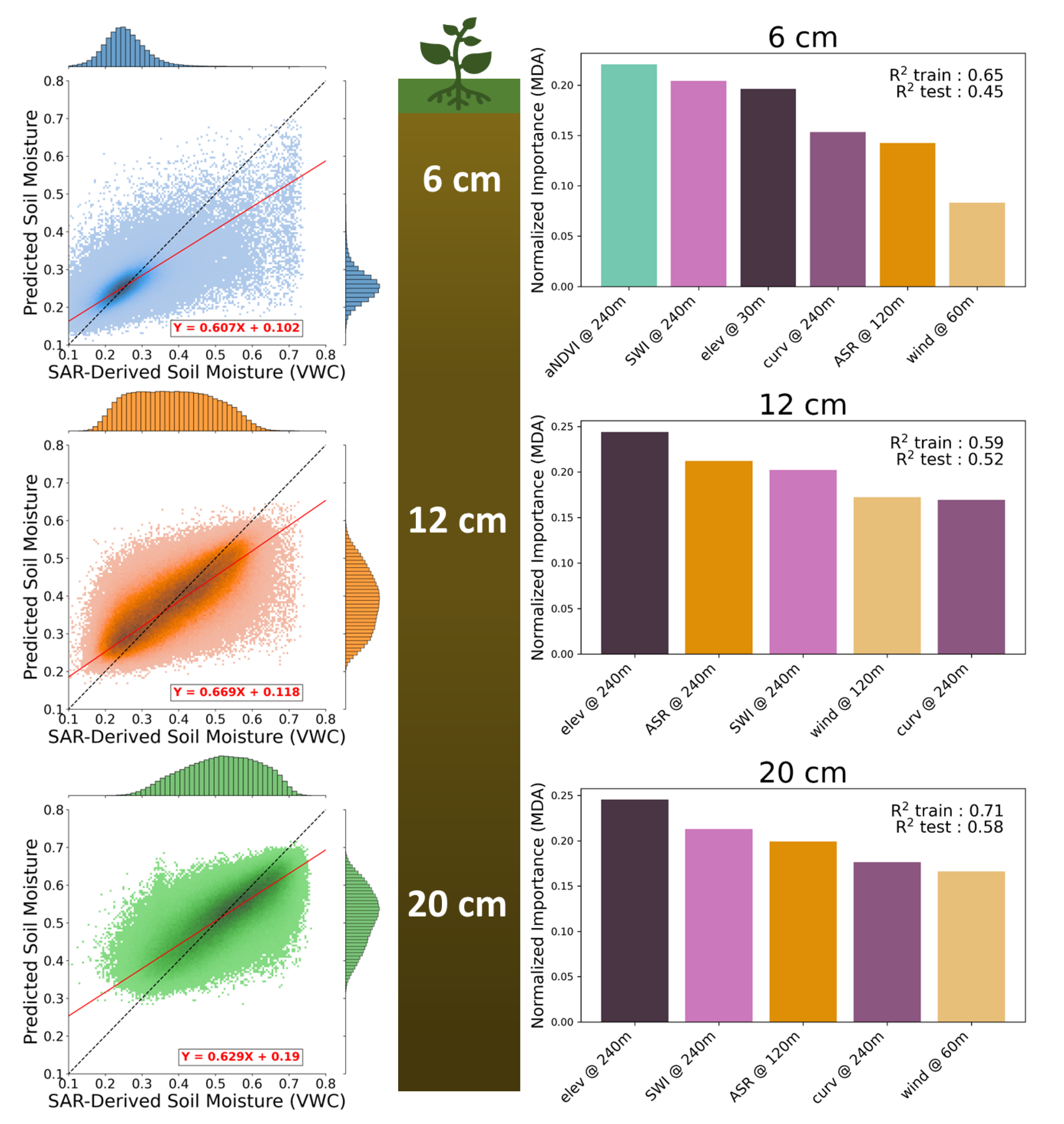
Figure 1. The main map illustrates the two footprints of the P-band SAR flight swaths over the Seward Peninsula (outlined in red). Shown within the flight footprints are dominant land cover types from the 2016 Alaska NLCD. The Teller Site, located at mile marker 27 of the Nome-Teller Highway, is highlighted in black. Inset shows all 2017 AirMOSS (P-Band) SAR footprints flown by the NASA ABoVE campaign over Alaska and Canada.
Remotesensing 14 04927 g001
Figure 2. An example soil profile for a given pixel of the Chen et al. (2019) product. Each pixel has a surface roughness h, which is constant between the August and October SAR backscatter retrievals. The saturated active layer has a consistent dielectric (𝛆2) constant that depends only on the soil porosity. Between retrievals of the SAR instrument, the depth of the unsaturated surface layer (Z1) and the dielectric constant of the unsaturated surface layer(𝛆1) change. Z2 is the depth of the active layer which is assumed to not vary substantially between maximum thaw (August) and partially frozen (October) in which most of the freezing occurs from the top down. The square labeled ‘TL_SAR_4’ is a ground-truthing plot established by the Next Generation Ecosystem Experiment Arctic (NGEE Arctic) with labeled points representing in situ soil moisture observations. Figure is adapted from Chen et al., 2019, Figure 3 [41].
Remotesensing 14 04927 g002
Figure 3. Steps in the fitting procedure to go from using all features and resolutions to a final model for each depth. In parentheses is the method used for each step. CV is the number of cross-validations applied at. N is the number of combinations for the grid search. VIF is the variance inflation factor.
Remotesensing 14 04927 g003
Figure 4. The impact of the number of trees (left) and the max depth of individual trees (right) on the R2 of the test data set (20 cm).
Remotesensing 14 04927 g004
Figure 5. Hierarchical clustering dendrogram based on Ward’s method (left) [79] and Pearson’s correlation matrix (right) of the ten predictor features at the highest resolution considered in this study. Four main clusters are identified: vegetation features: NDVI, EVI, and TCG; major topography features: elevation, slope, and SWI; minor topography features: curvature and TPI, and meteorological features: ASR and the wind factor.
Remotesensing 14 04927 g005
Figure 6. Distribution of SAR-derived volumetric water content for 6 cm, 12 cm, and 20 cm depths. The shaded histogram represents the SAR-derived soil moisture values and the lines are the associated random forest predictions for each depth.
Remotesensing 14 04927 g006
Figure 7. Results of a recursive feature elimination based on feature scales identified in the all-feature model. In the left-hand plots, we show an increase in the R2 of the test scores as the number of features increases. The dashed red line indicates a threshold of 2.5% used to identify the number of features used in the final model for each depth. The right-hand side plots show the permutation feature importance (MDA) for the features included in each model fitting stage. We show plots for 6 cm, 12 cm, and 20 cm soil depths.
Remotesensing 14 04927 g007
Figure 8. Relationship between SAR-derived soil moisture and random forest soil moisture predictions at 6 cm, 12 cm, and 20 cm. The dashed black line is the 1:1, the solid red line is the result of a robust linear regression (Huber), distributions for both the predicted and SAR-derived soil moisture are shown on the sides of the plot. On the right side of the figure are feature importances (MDA) for input features for the final fits at each depth in the soil column.
Remotesensing 14 04927 g008
Table 1. Final random forest model parameters and scores.
DepthFeatures (In Order of Decreasing Permutation Importance)Train R2Test R2
6 cmNDVI @240 m, SAGA Wetness Index @240 m, Elevation @30 m, Curvature @240 m, Areal Solar Radiation @120 m, Wind Factor @60 m0.6540.447
12 cmElevation @240 m, Areal Solar Radiation @240 m, SAGA Wetness Index @240 m, Wind Factor @120 m, Curvature @240 m0.5870.517
20 cmElevation @240 m, SAGA Wetness Index @240 m, Areal Solar Radiation @120 m, Curvature @240 m, Wind Factor @60 m0.7130.576
Publisher’s Note: MDPI stays neutral with regard to jurisdictional claims in published maps and institutional affiliations.

