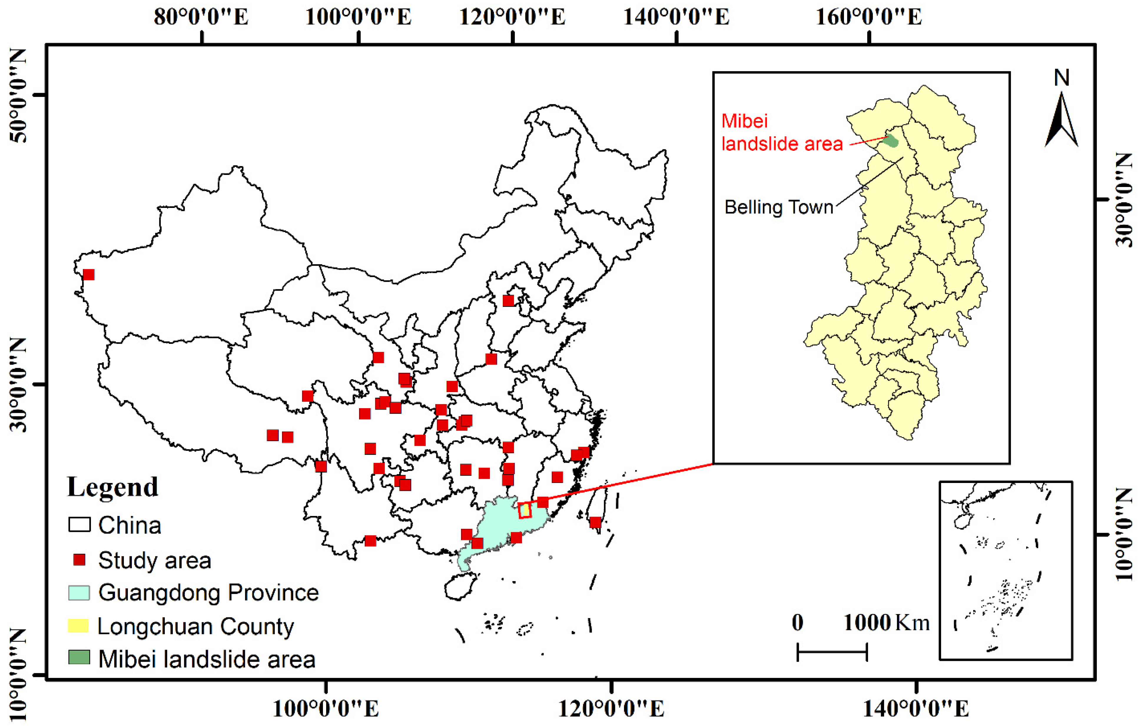
Figure 1.
The location of the study area. The red rectangular boxes are landslide study areas, with multiple landslides distributed within each area.
Figure 1.
The location of the study area. The red rectangular boxes are landslide study areas, with multiple landslides distributed within each area.
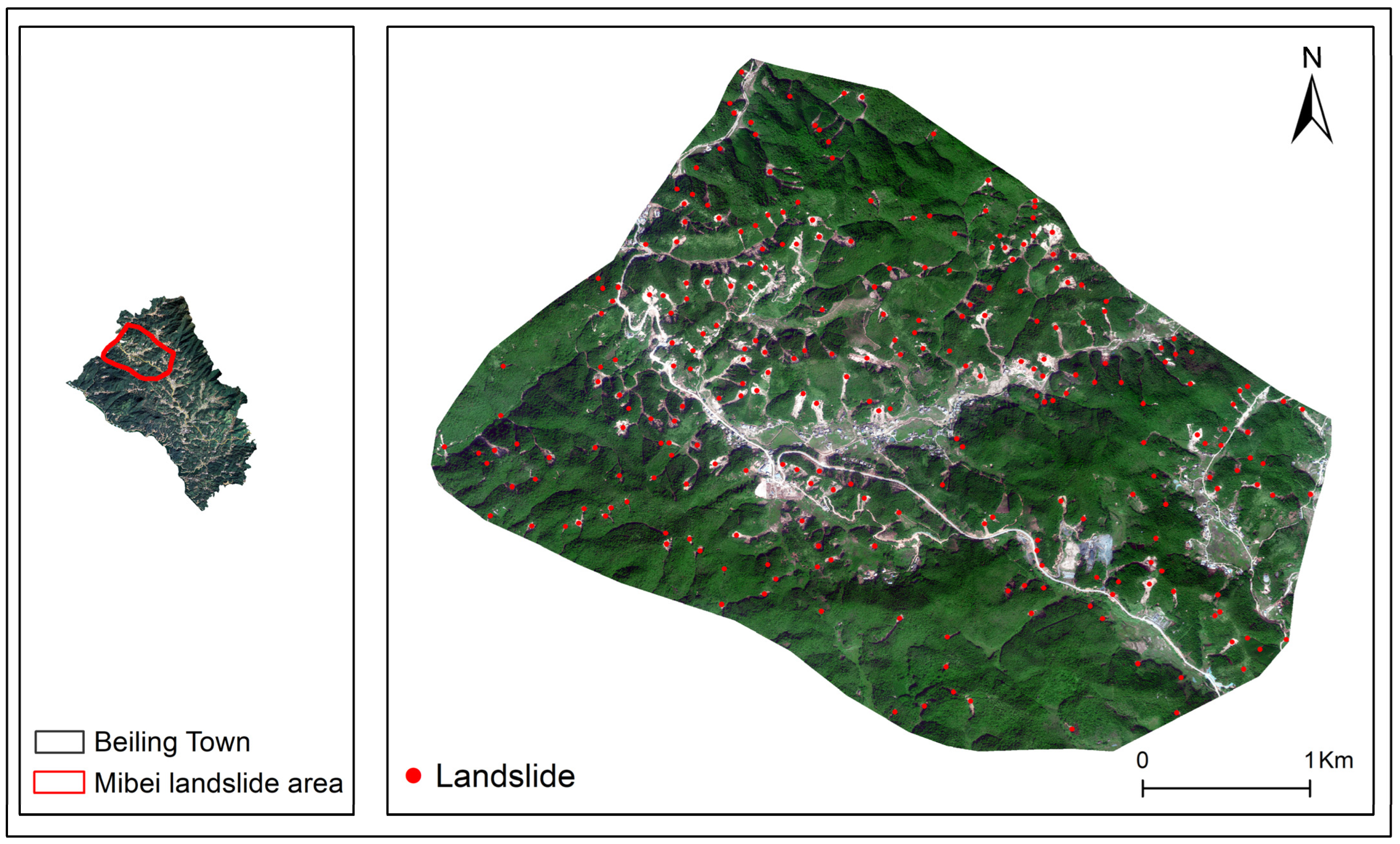
Figure 2.
The landslide area is located in Mibei Village, Beiling Town, Longchuan County, Heyuan City, Guangdong Province, China. The red points are the locations of landslides identified after the survey.
Figure 2.
The landslide area is located in Mibei Village, Beiling Town, Longchuan County, Heyuan City, Guangdong Province, China. The red points are the locations of landslides identified after the survey.
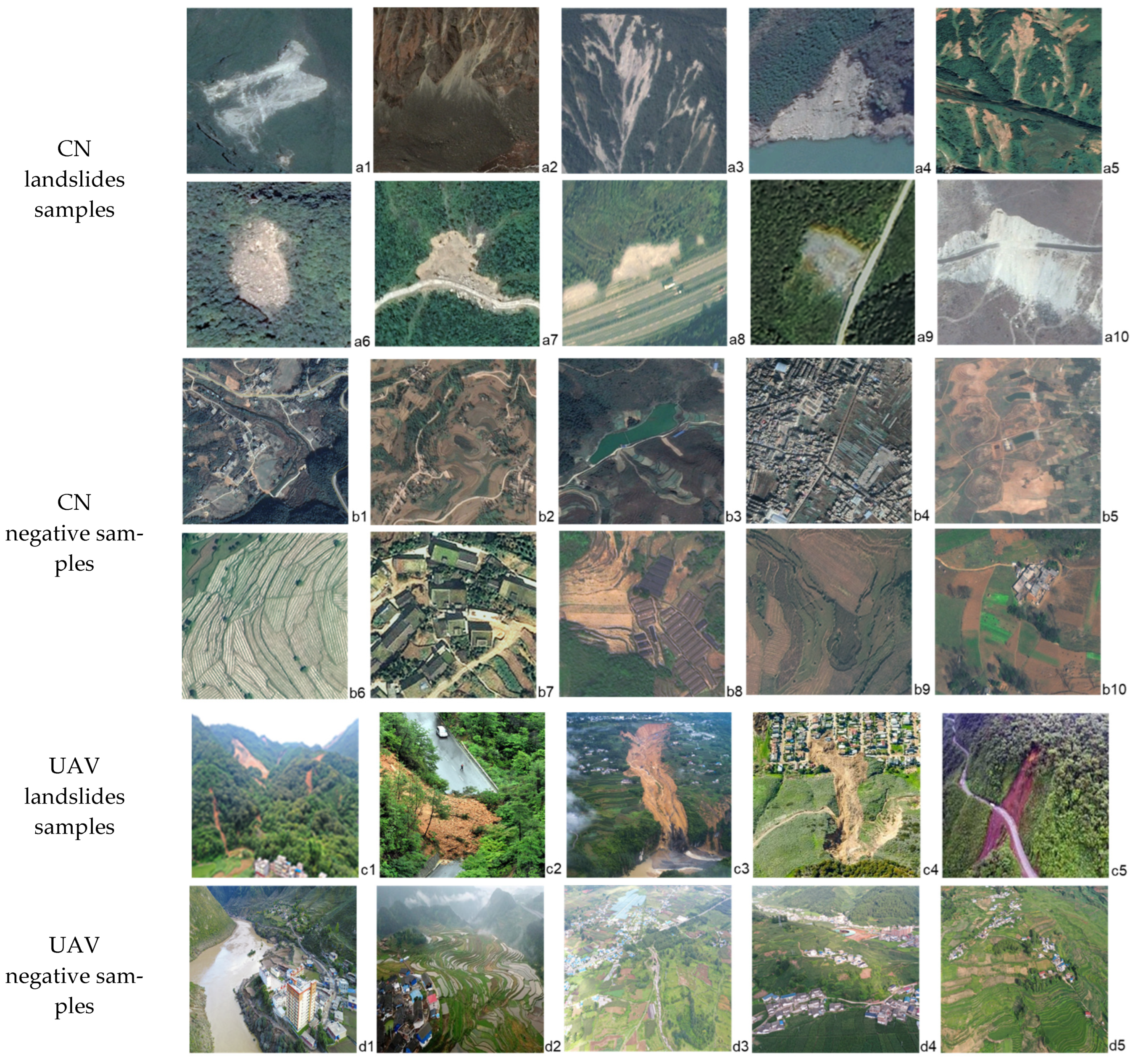
Figure 3.
The research sample for this paper. The landslide samples contain one or more landslides per image, and the negative samples are environmental images that do not contain landslides. CN landslides samples: (a1–a10); CN negative samples: (b1–b10); UAV landslides samples: (c1–c5); UAV negative samples: (d1–d5).
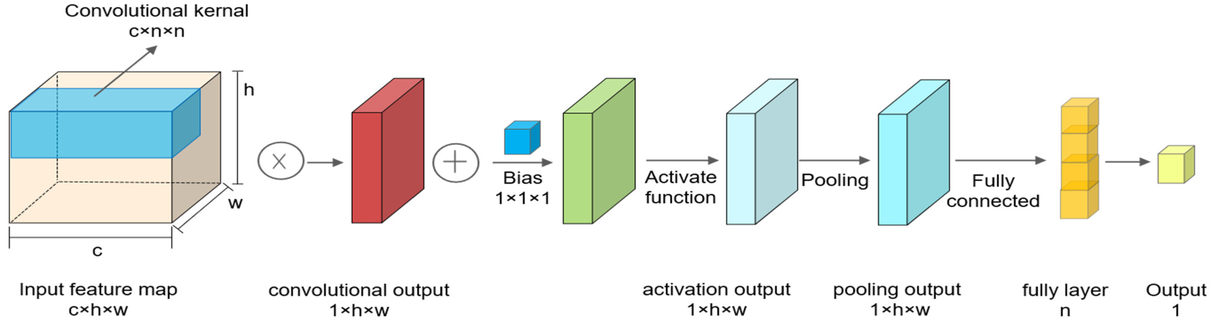
Figure 4.
The basic CNN structure. The “×” and “+” with circles are multiplication and addition operations.
Figure 4.
The basic CNN structure. The “×” and “+” with circles are multiplication and addition operations.
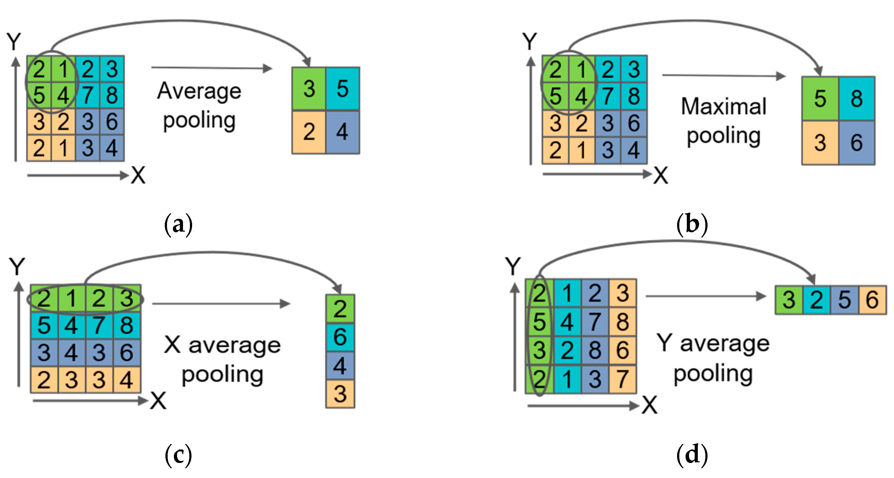
Figure 5.
Four typical pooling operations: (a) Average pooling; (b) Maximal pooling; (c) X average pooling: one-dimensional features are encoded along the horizontal direction and then aggregated along the vertical direction; (d) Y average pooling: one-dimensional features are encoded along the vertical direction and then aggregated along the horizontal direction.
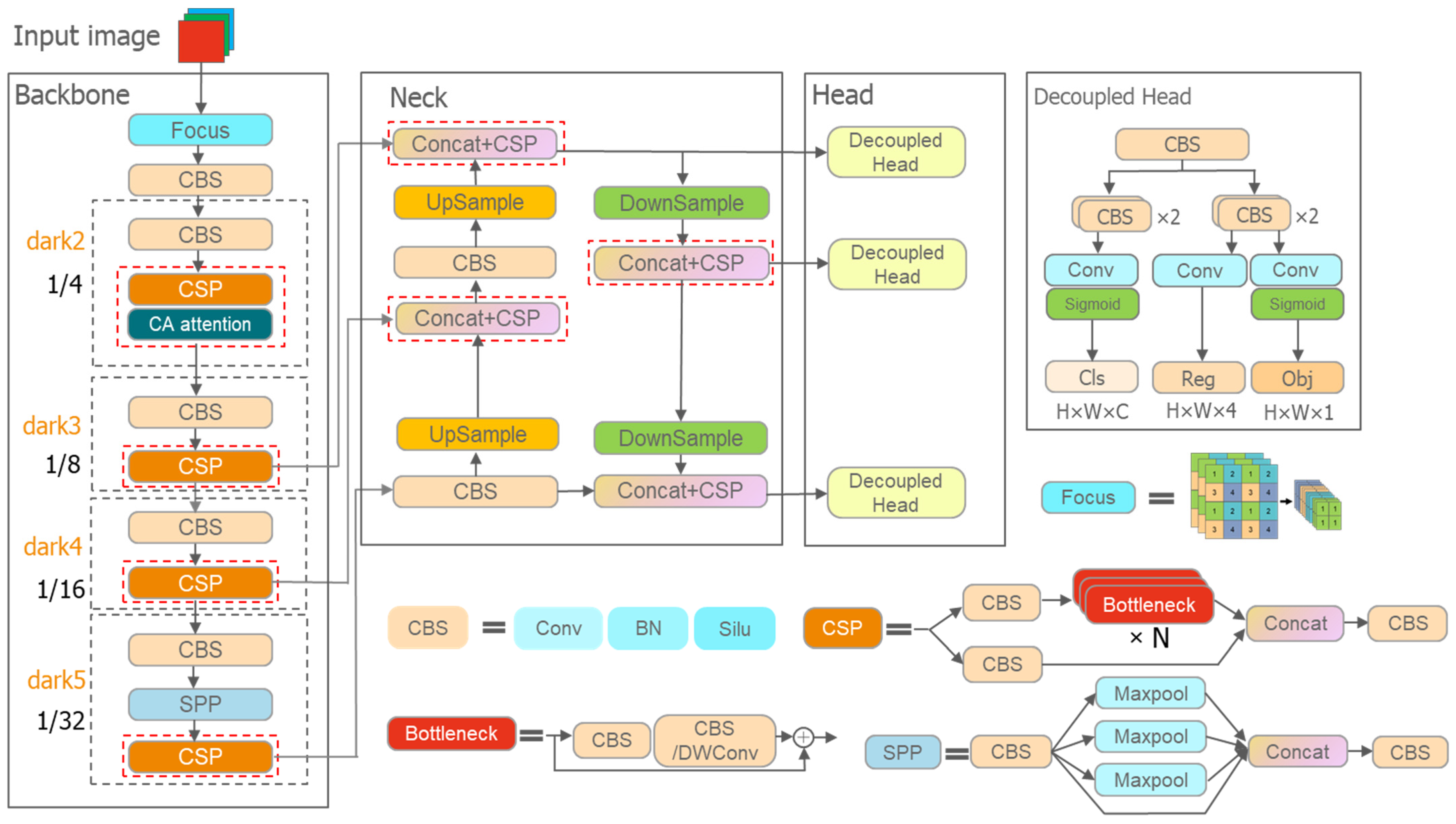
Figure 6.
YOLOX network structure. The red dotted boxes are the alternative locations for adding the attention module. The Conv, BN, and Silu denote Convolution, Batch Normalization, and SILU, respectively. The Concat and Maxpool denote Concatenation and Maximum pooling operations. The DWConv is a variant of the Convolution operation. The Cls, Reg, and Obj represent the classification, the regression parameters of each feature point, and the detected target’s confidence score information from the input image. The prediction box can be obtained by adjusting the regression parameters. The confidence score represents the probability that each feature point prediction box contains an object. The H, W, and X indicate the feature maps’ width, height, and number of channels.
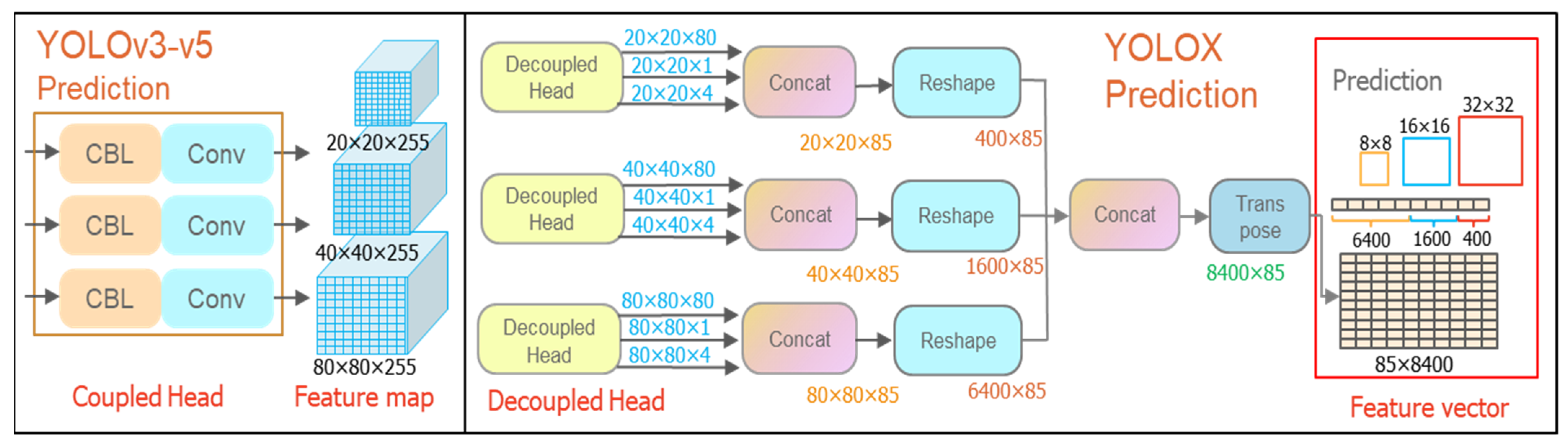
Figure 7.
YOLO series detection head structure. The CBL module consists of Convolution, Batch Normalization, and LeakyRelu functions to extract and transform the input features, where a is a tiny constant. The number of prediction boxes corresponding to the three types of feature points is 6400, 1600, and 400, respectively.
Figure 8.
Model design flowchart.
Figure 8.
Model design flowchart.
Figure 9.
The Coordinate Attention workflow. C, H, and W are the number of channels, height, and width of the feature map, respectively. The r denotes the compression ratio of the channels.
Figure 9.
The Coordinate Attention workflow. C, H, and W are the number of channels, height, and width of the feature map, respectively. The r denotes the compression ratio of the channels.
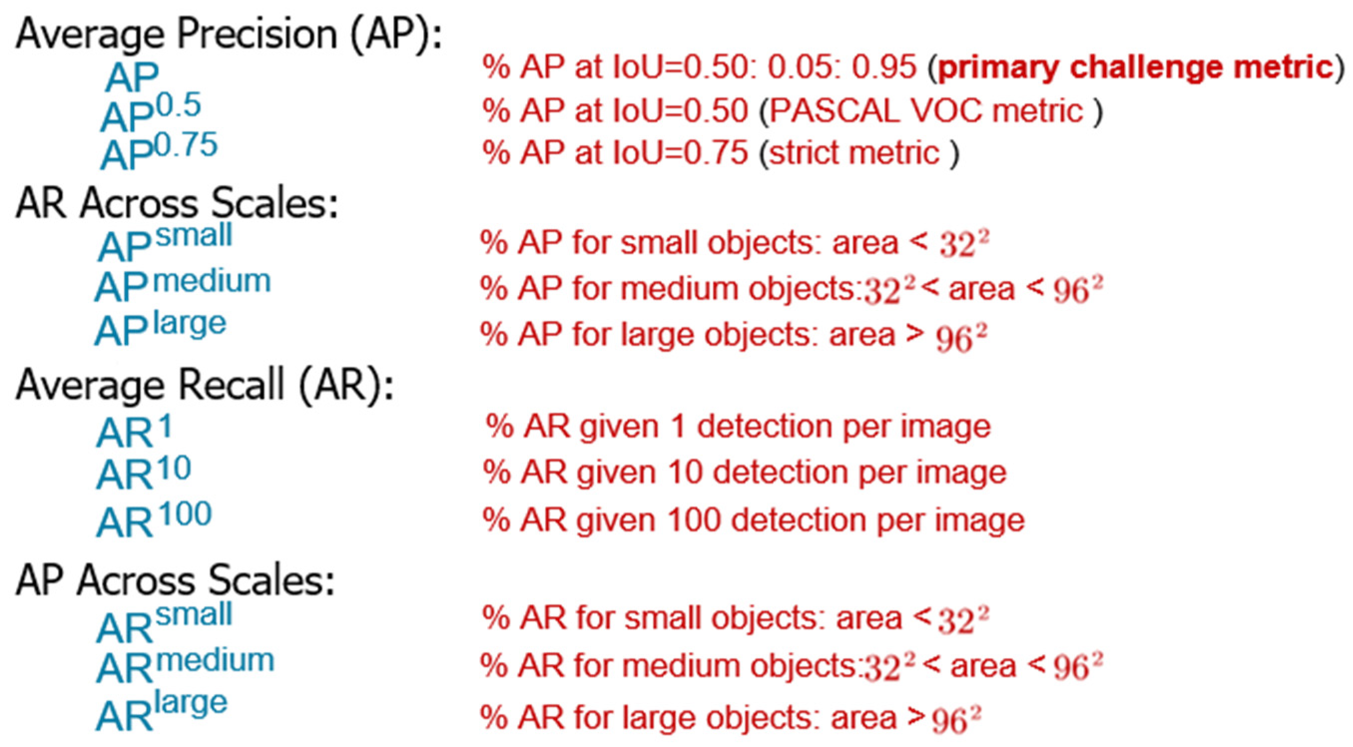
Figure 10.
The detection evaluation metrics of COCO.
Figure 10.
The detection evaluation metrics of COCO.
Figure 11.
The workflow of landslide detection from CN dataset, UAV dataset, and Mibei landslide area.
Figure 11.
The workflow of landslide detection from CN dataset, UAV dataset, and Mibei landslide area.
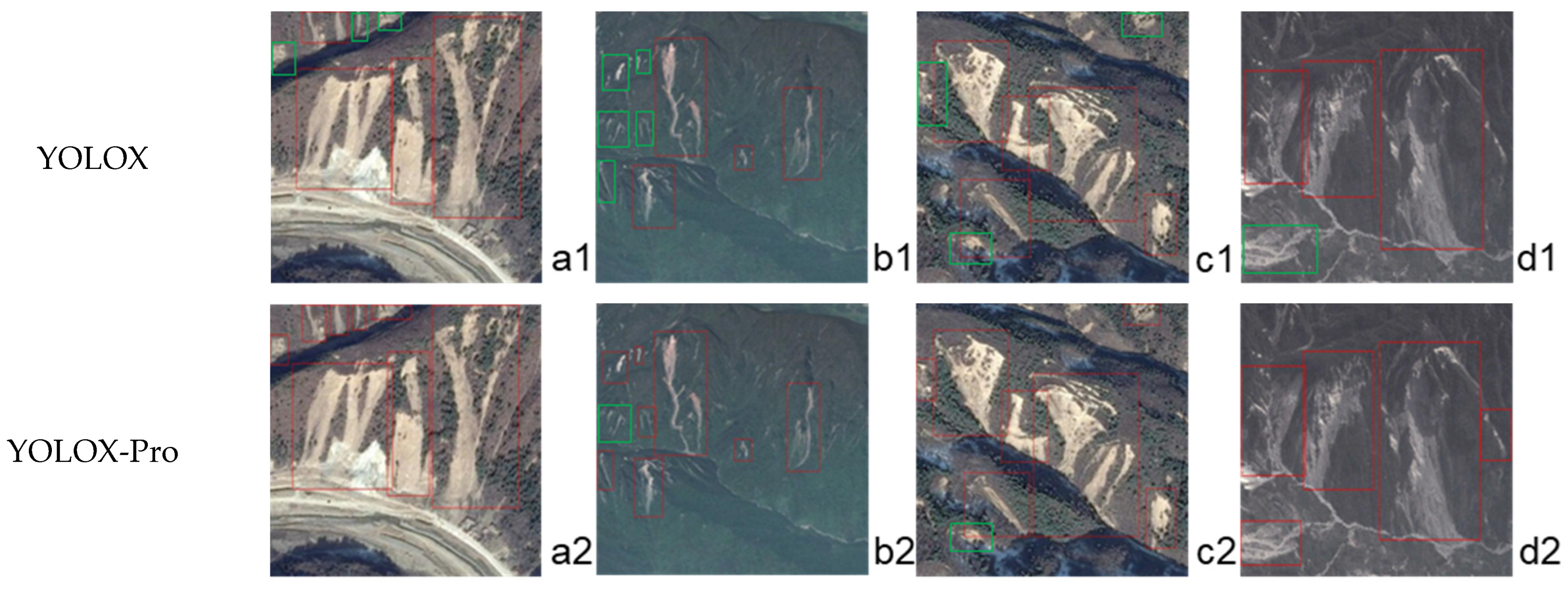
Figure 12.
Comparison of detection results of YOLOX(M) and YOLOX-Pro(M) models. The red target boxes indicate the landslides automatically detected by the model, and the green target boxes are the manually labeled missed landslides. (a1–c1): the detection effect of small landslides is poor, and there are many missed detections; d1: the debris flow in the lower left corner of the image was missed; (a2–d2): better detection performance, least missed detection.
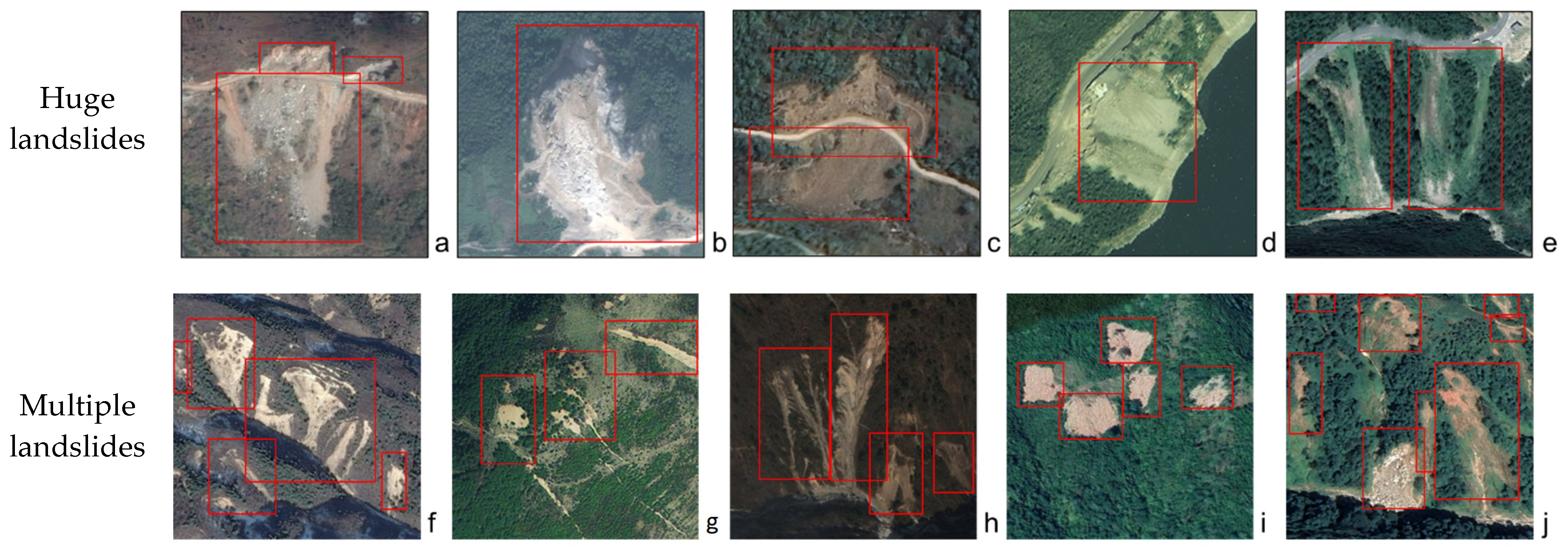
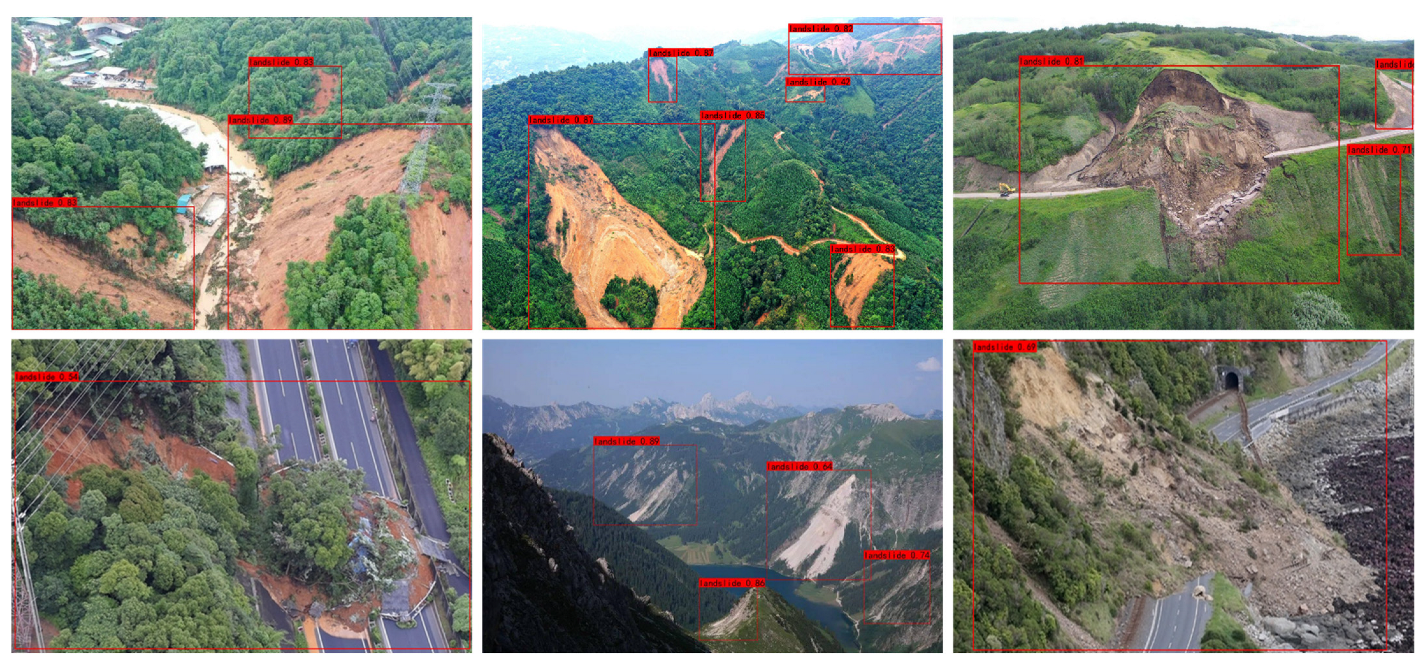
Figure 13.
Detection results of potential landslide areas by YOLOX-Pro(M). The partially representative detection results of YOLOX-Pro for potential landslide areas. The red rectangles mark the boundaries of the landslide, which the model automatically detects. (Huge landslides) (a–e): the huge landslides. (Multiple landslides) (f–j): the multiple landslides of different sizes; (Complex landslides) (k,l): the historical landslides areas are very similar to the surrounding environment; (m–o): the landslides that have been covered by surface vegetation in some areas. (Small landslides) (p–t): the small landslides along the road.
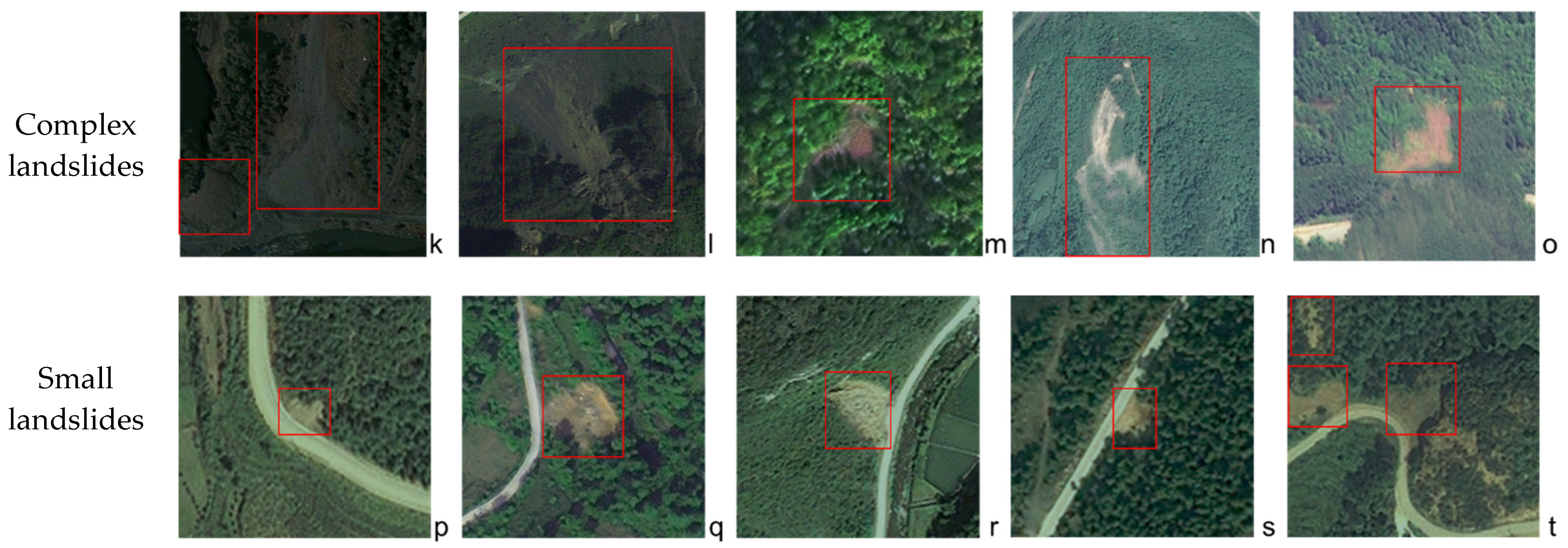
Figure 14.
Detection results of Mibei area by YOLOX-Pro(M). (a,b,d): Detection results of dense areas of landslides. (c): Landslide detection results for the Mibe area. The red, blue, and yellow points indicate the correct, erroneous, and missed landslide detection locations, respectively. The red rectangles mark the landslide boundaries, which the model automatically detects. The yellow and blue rectangular boxes are the model’s missed and erroneously detected landslides, respectively.
Figure 15.
Detection results of UAV landslide image area by YOLOX-Pro(M).
Figure 15.
Detection results of UAV landslide image area by YOLOX-Pro(M).
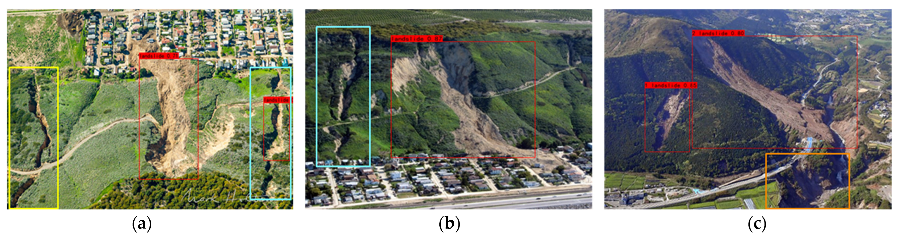
Figure 16.
(a): The yellow box is the landslide fissure, and the blue box is the landslide detected after converting the angle; (b): the blue box is the missed landslide; (c): the orange box is the missed landslide.
Figure 16.
(a): The yellow box is the landslide fissure, and the blue box is the landslide detected after converting the angle; (b): the blue box is the missed landslide; (c): the orange box is the missed landslide.
Table 1.
The dataset in this paper. Each sample is an image, the landslide sample contains one to more landslides, and there are no landslides in the negative sample.
Table 1.
The dataset in this paper. Each sample is an image, the landslide sample contains one to more landslides, and there are no landslides in the negative sample.
| Dataset | Images | Total Images |
|---|
| CN dataset | 1200 landslides samples | 720 earth slides | 2400 |
| 400 rock slides |
| 80 debris flows |
| 1200 negative samples |
| UAV dataset | 250 landslides samples | 750 |
| 500 negative samples |
Table 2.
The Parameters of YOLOX and YOLOX-Pro.
Table 2.
The Parameters of YOLOX and YOLOX-Pro.
| | Parameters (Mb) |
|---|
| Network Size | Nano | Tiny | S | M | L |
| YOLOX | 0.91 | 5.06 | 9.00 | 25.30 | 54.20 |
| YOLOX-Pro | 1.42 | 6.51 | 10.30 | 26.50 | 57.51 |
Table 3.
The details of dataset division. The UAV dataset does not have validation set. The Mibei landslide area is only divided into test set for landslide detection.
Table 3.
The details of dataset division. The UAV dataset does not have validation set. The Mibei landslide area is only divided into test set for landslide detection.
| | CN Dataset | UAV Dataset | Mibei Landslide
Area |
|---|
| Data Composition | Landslide images | Negative images | Landslide images | Negative images | images |
| Train | 770 | 670 | 150 | 400 | - |
| Val | 180 | 300 | - | - | - |
| Test | 250 | 230 | 100 | 100 | 26 |
| Total | 1200 | 1200 | 250 | 500 | 26 |
Table 4.
The effect of different attentional mechanisms on the YOLOX-Pro model.
Table 4.
The effect of different attentional mechanisms on the YOLOX-Pro model.
| Model | Params (Mb) | AP (%) | AP0.75 (%) | APsmall (%) | ARsmall (%) |
|---|
| YOLOX (m) | 25.30 | 47.00 | 48.30 | 32.50 | 46.80 |
| YOLOX-CA (m) | 26.50 | 47.80 | 51.50 | 36.50 | 49.50 |
| YOLOX-CBAM (m) | 26.68 | 47.70 | 50.10 | 35.30 | 47.90 |
| YOLOX-SE (m) | 26.59 | 47.50 | 49.80 | 35.70 | 48.10 |
| YOLOX (nano) | 0.91 | 45.10 | 44.60 | 31.30 | 45.00 |
| YOLOX-CA (nano) | 1.42 | 46.10 | 46.90 | 33.70 | 47.50 |
| YOLOX-CBAM (nano) | 1.44 | 45.70 | 46.70 | 33.10 | 47.20 |
| YOLOX-SE (nano) | 1.43 | 45.60 | 46.60 | 32.80 | 46.90 |
Table 5.
Comparison of detection performance of different models.
Table 5.
Comparison of detection performance of different models.
| Model | Params (Mb) | AP0.5 (%) | Recall (%) | Precision (%) |
|---|
| YOLOX-Pro (m) | 26.50 | 84.85 | 81.52 | 85.36 |
| YOLOX (m) | 25.30 | 81.73 | 75.09 | 82.30 |
| YOLOv5 (m) | 21.20 | 74.30 | 68.95 | 80.25 |
| Faster R-CNN (resnet-50) | 107.87 | 71.35 | 77.37 | 67.56 |
| SSD (vgg) | 90.07 | 69.15 | 57.29 | 76.19 |
Table 6.
Comparison of detection performance between YOLOX and YOLOX-Pro models.
Table 6.
Comparison of detection performance between YOLOX and YOLOX-Pro models.
| | YOLOX | YOLOX-Pro |
|---|
| | l | m | s | Tiny | Nano | l | m | s | Tiny | Nano |
|---|
| Params (Mb) | 54.20 | 25.30 | 9.00 | 5.06 | 0.91 | 57.51 | 26.50 | 10.30 | 6.51 | 1.42 |
| AP (%) | 47.20 | 47.00 | 45.30 | 45.10 | 45.10 | 48.30 | 47.80 | 47.00 | 46.70 | 46.10 |
| AP0.75 (%) | 48.70 | 48.30 | 45.00 | 45.20 | 44.60 | 52.40 | 51.50 | 50.80 | 48.80 | 46.90 |
| APsmall (%) | 33.40 | 32.50 | 32.10 | 31.40 | 31.30 | 37.50 | 36.50 | 35.30 | 34.82 | 33.70 |
| ARsmall (%) | 47.00 | 46.80 | 45.70 | 45.40 | 45.00 | 49.80 | 49.50 | 49.20 | 48.60 | 447.50 |
| AR10 (%) | 58.60 | 58.60 | 57.70 | 57.80 | 57.40 | 61.70 | 61.20 | 60.90 | 60.50 | 60.10 |
Table 7.
Results of the YOLOX-Pro network for detecting the Mibei area.
Table 7.
Results of the YOLOX-Pro network for detecting the Mibei area.
| Model | Params (Mb) | AP0.5 (%) | Recall (%) | Precision (%) |
|---|
| YOLOX-Pro (l) | 57.51 | 85.19 | 86.76 | 83.95 |
| YOLOX-Pro (m) | 26.50 | 83.77 | 83.88 | 81.37 |
| YOLOX-Pro (s) | 10.30 | 81.86 | 82.51 | 80.86 |
| YOLOX-Pro (tiny) | 6.51 | 80.55 | 80.22 | 80.35 |
| YOLOX-Pro (nano) | 1.42 | 79.30 | 79.18 | 79.56 |
Table 8.
Results of the YOLOX-Pro network for detecting the UAV dataset.
Table 8.
Results of the YOLOX-Pro network for detecting the UAV dataset.
| Model | Params (Mb) | AP0.5 (%) | Recall (%) | Precision (%) |
|---|
| YOLOX-Pro (l) | 57.51 | 86.35 | 83.51 | 84.65 |
| YOLOX-Pro (m) | 26.50 | 85.87 | 82.37 | 83.28 |
| YOLOX-Pro (s) | 10.30 | 84.56 | 81.77 | 82.54 |
| YOLOX-Pro (tiny) | 6.51 | 83.28 | 80.82 | 81.66 |
| YOLOX-Pro (nano) | 1.42 | 82.47 | 80.36 | 80.88 |
Table 9.
The effect of the location and quantity of CA modules on the base model. The YOLOX model with the VariFocal loss function was used as the base model for this experiment.
Table 9.
The effect of the location and quantity of CA modules on the base model. The YOLOX model with the VariFocal loss function was used as the base model for this experiment.
| Description | Params (Mb) | AP | AP0.75 | APsmall | ARsmall |
|---|
| base model(m) | 26.50 | 47.50 | 49.50 | 34.90 | 47.80 |
| YOLOX -CA _dark2(m) | 26.50 | 47.80 | 51.50 | 35.80 | 49.50 |
| YOLO -CA _dark3–5(m) | 26.58 | 46.80 | 50.40 | 33.50 | 49.20 |
| YOLOX -CA _neck(m) | 26.55 | 47.40 | 49.90 | 34.70 | 48.50 |
| base model (nano) | 1.40 | 45.50 | 46.60 | 32.50 | 46.70 |
| YOLOX -CA _dark2(nano) | 1.42 | 45.90 | 46.90 | 33.70 | 47.50 |
| YOLOX -CA _dark3–5(nano) | 1.44 | 44.60 | 46.80 | 31.20 | 47.50 |
| YOLOX -CA _neck(nano) | 1.44 | 45.30 | 46.60 | 31.90 | 47.40 |


