
A Novel Lidar Signal-Denoising Algorithm Based on Sparrow Search Algorithm for Optimal Variational Modal Decomposition

Abstract
:1. Introduction
2. Methodology
2.1. Lidar Equation
2.2. VMD Algorithm
2.3. Sparrow Search Algorithm (SSA)
2.4. SVD Algorithm
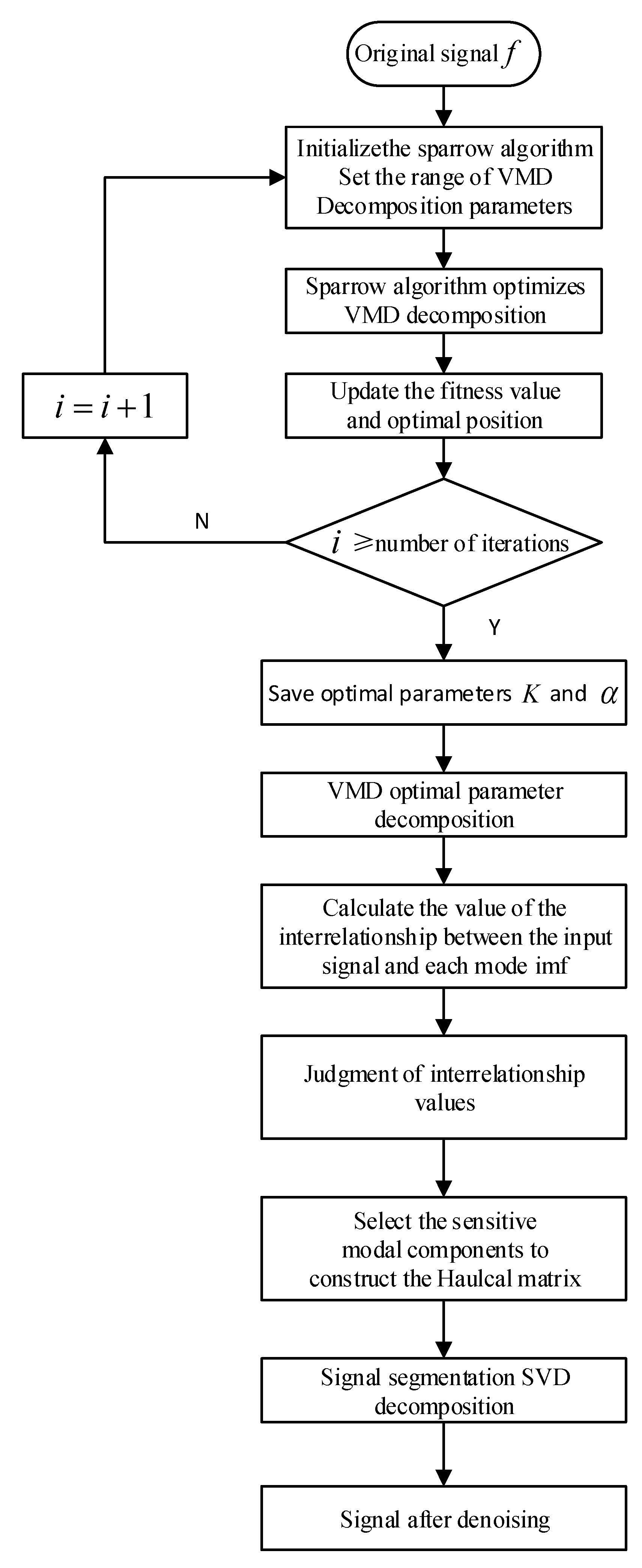
2.5. VMD-SSA-SVD Noise-Reduction Method
- (1)
- The signal is acquired and the optimal combination for penalty parameters α and modal numbers is found by using the VMD-SSA algorithm.
- (2)
- The signal undergoes VMD according to the parameters of (1).
- (3)
- The interrelationship number of each IMF component and the original signal is calculated, the interrelationship number threshold is determined, and the component greater than or equal to the threshold is selected as the sensitive modal component.
- (4
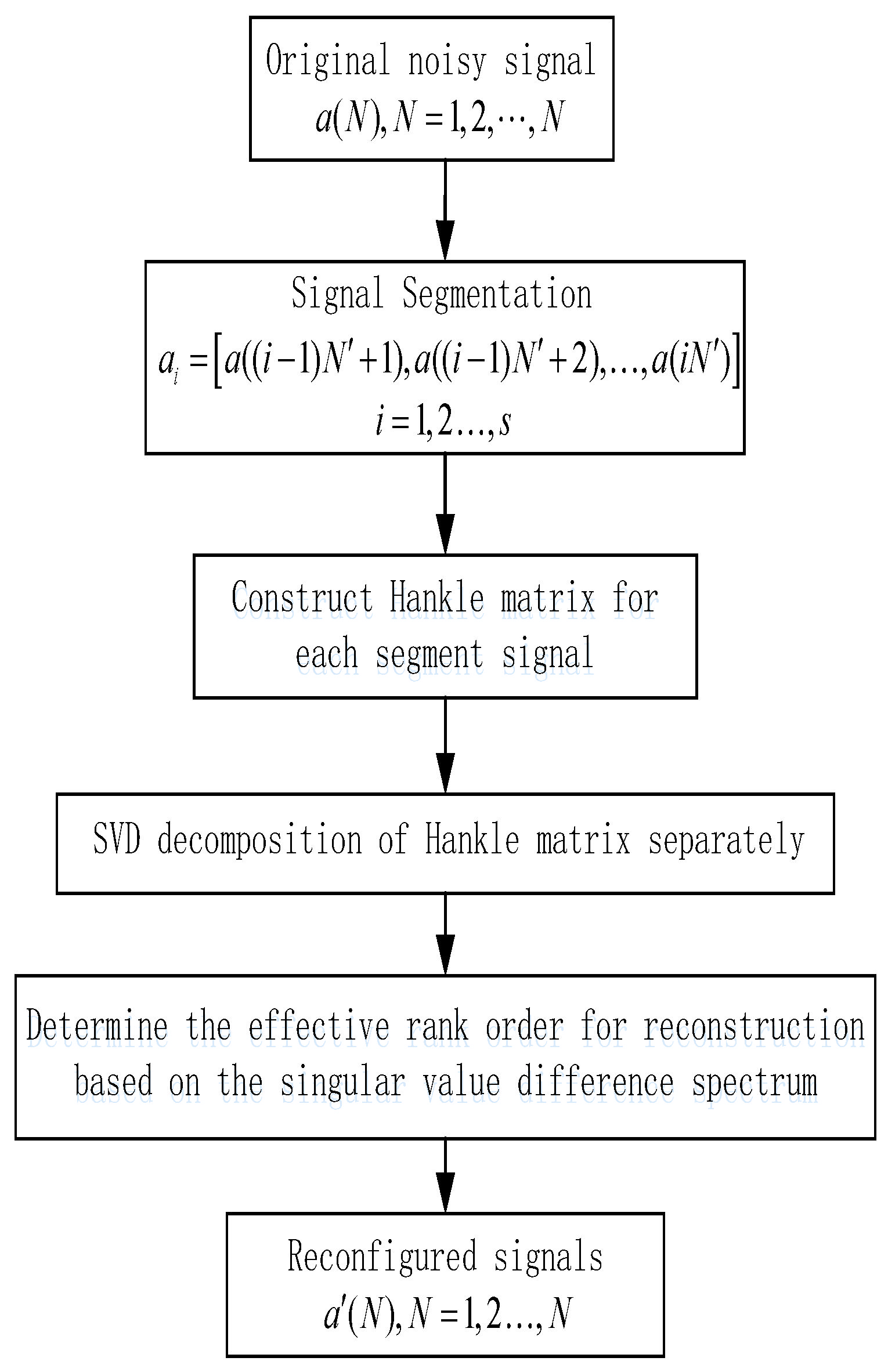
- The Hankel matrix of the sensitive modal component signal is obtained, SVD is performed, signal segmentation SVD noise-reduction processing is used, the effective order of the SVD is determined, and noise-reduction processing on the sensitive modal component through SVD is performed.
- (5)
- The modal components of the SVD are reconstructed to obtain the final noise-reduction signal.
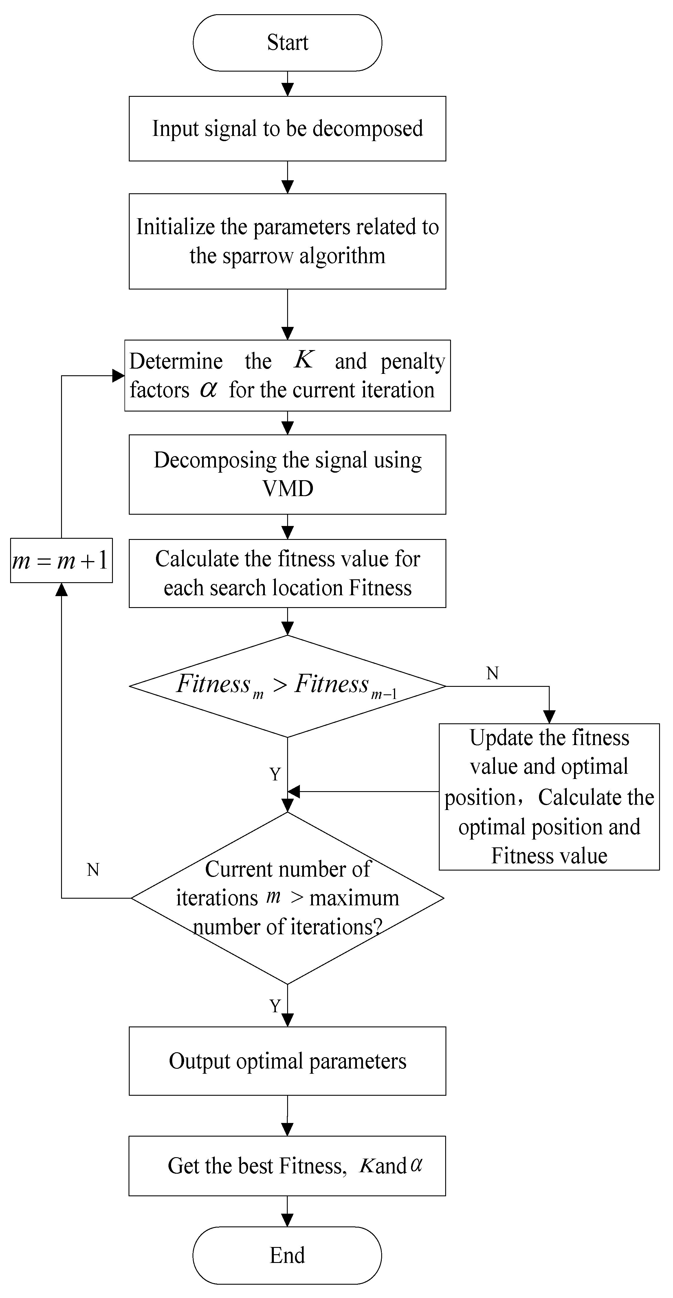
2.5.1. Optimizing VMD Based on the SSA
- (1)
- In the case of the original signal input, f, the range of values of VMD parameters is determined, and the model parameters of SSA are set and initialized, which include the maximum number of iterations and the initial population number. The fitness function is the local minimal envelope entropy. In this paper, takes the integer in the interval [2, 15], takes the integer in the interval [1000, 10,000], and the maximum number of iterations is set to 15. The number of populations is set to 30.
- (2)
- VMD of the signal and calculation of the initial fitness of each sparrow are next. Based on the optimization principle of the sparrow algorithm, the minimum fitness value is selected by updating the positions of the discoverer, the follower, and the position of the sparrow that is aware of the danger while continuously comparing the fitness values of each position.
- (3)
- Iterative loops are performed until the global optimal parameters and the best fitness values are determined or the maximum number of iterations is reached. The values are saved.
- (4)
- The previously obtained optimal parameters [,] are used to perform the VMD of the signal.
- (5)
- The interrelationship values of each modal component with the original signal are calculated.
- (6)
- The effective components for noise reduction are selected and reconstructed.
2.5.2. Selection of Effective Components Based on the Number of Interrelationships
2.5.3. SVD Segmentation Noise-Reduction Algorithm
3. Results and Discussion
3.1. Evaluation Index of the Noise-Reduction Effect
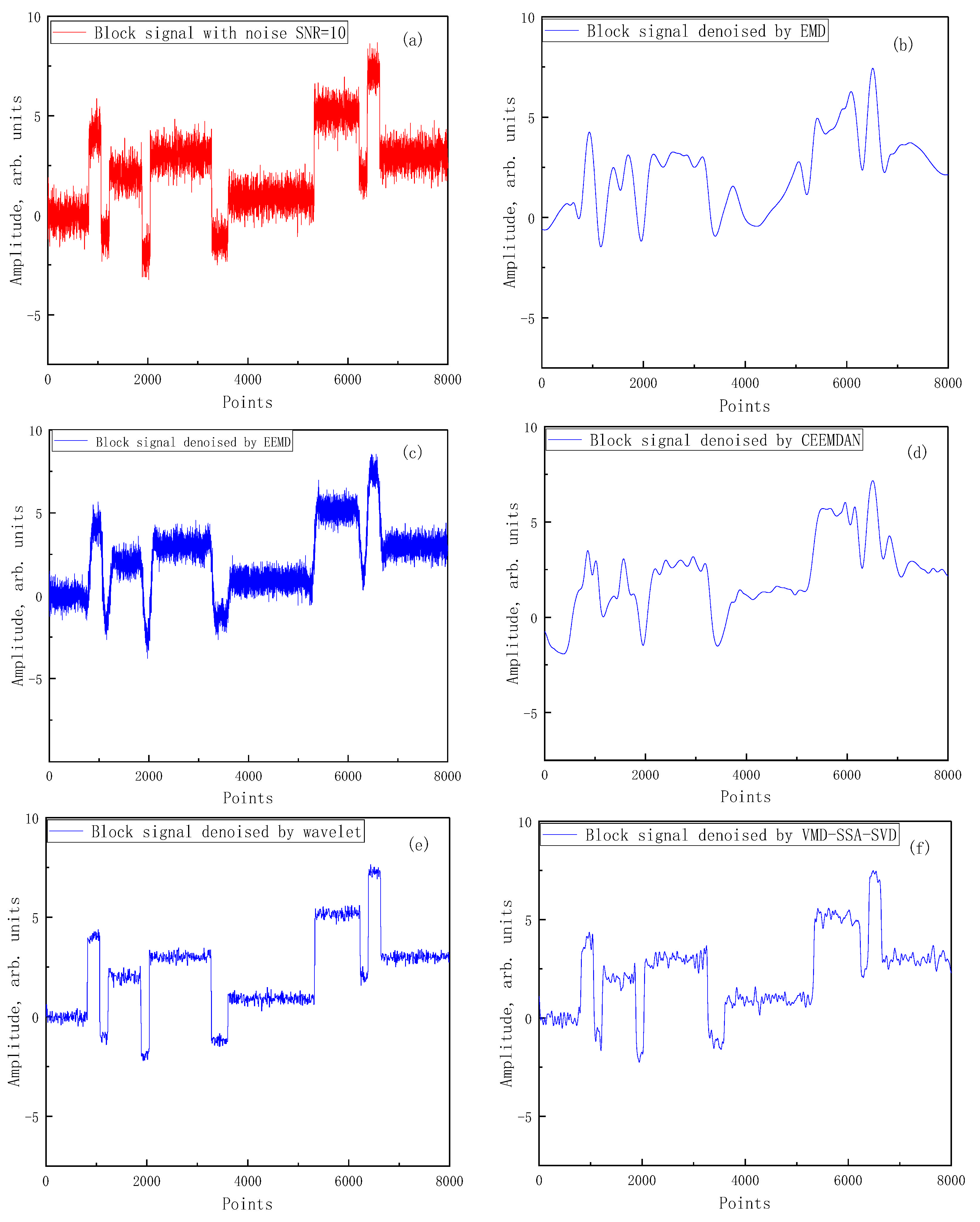
3.2. Simulation Signal Verification
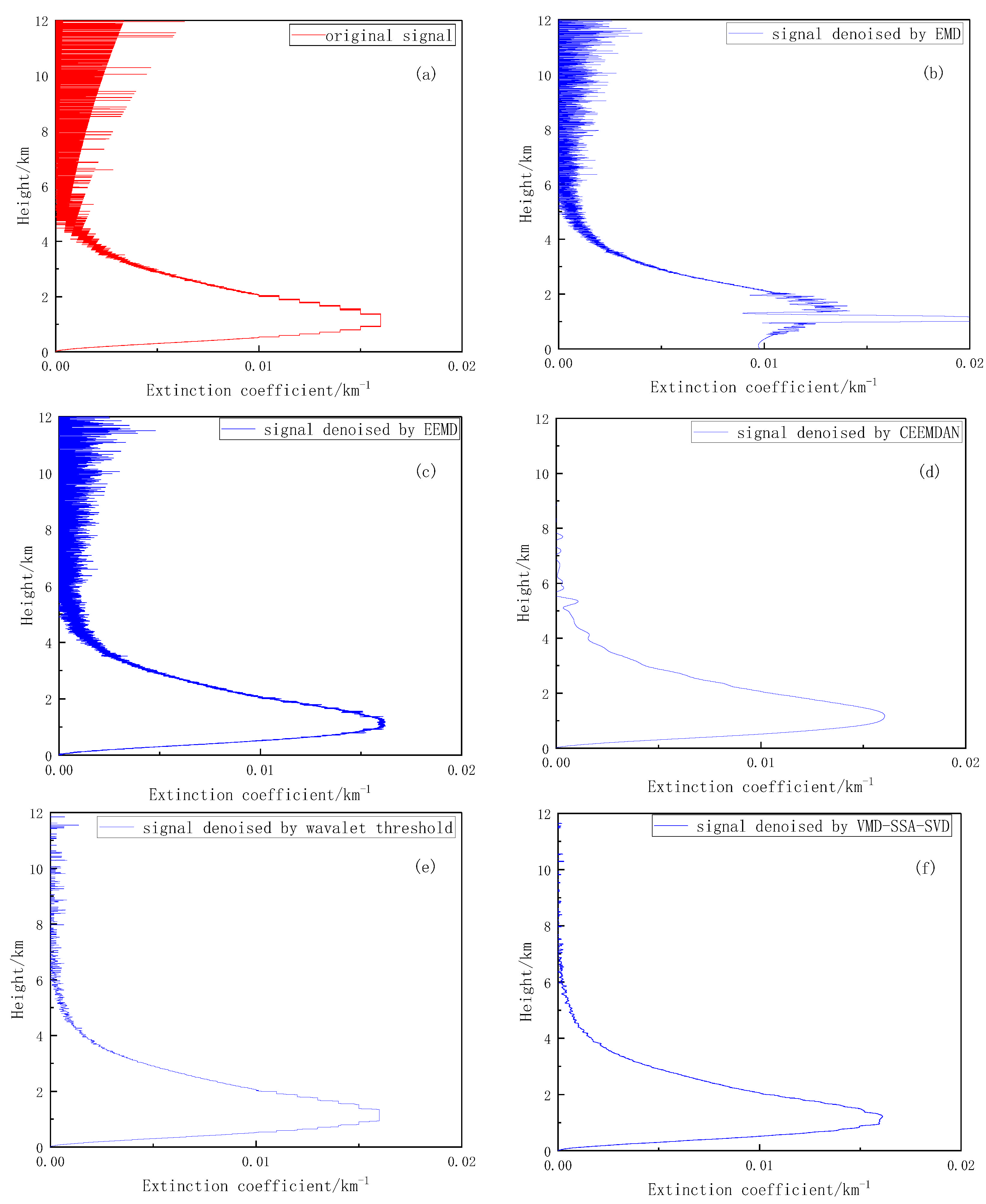
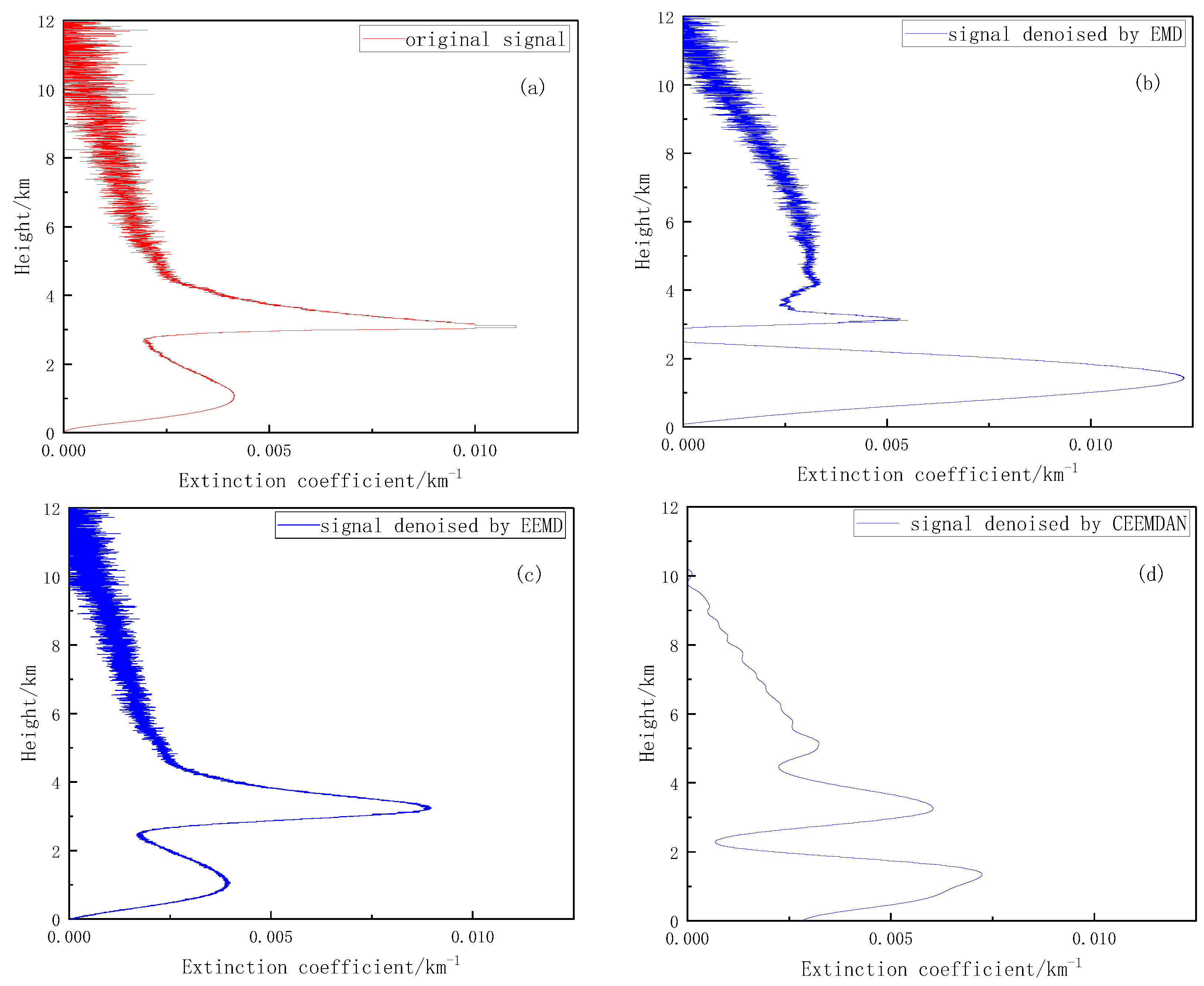
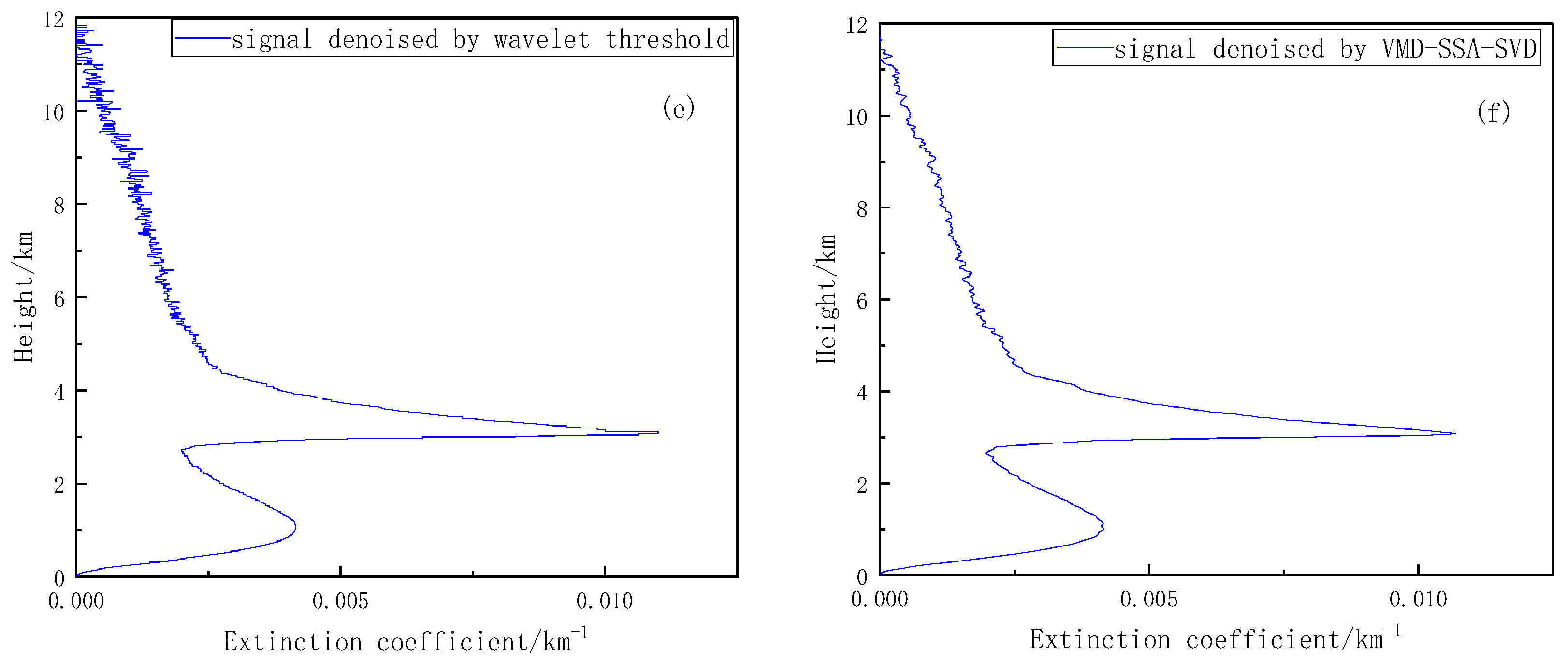
3.3. Comparison of Atmospheric Lidar-Measured Signal-Denoising Effect
4. Conclusions
Author Contributions
Funding
Institutional Review Board Statement
Informed Consent Statement
Data Availability Statement
Acknowledgments
Conflicts of Interest
References
- Fang, H.T.; Huang, D.S.; Wu, Y.H. Antinoise approximation of the lidar signal with wavelet neural networks. Appl. Opt. 2005, 44, 1077–1083. [Google Scholar] [CrossRef]
- Wu, S.; Liu, Z.; Liu, B. Enhancement of lidar backscatters signal-to-noise ratio using empirical mode decomposition method. Opt. Commun. 2006, 267, 137–144. [Google Scholar] [CrossRef]
- Wang, L. Wavelet transform-based lidar weak signal processing method. Master’s degree, Heilongjiang University, Heilongjiang, china, 2009. [Google Scholar]
- Mao, J.; Hua, D.; Wang, Y.; Wang, L. Noise Reduction in Lidar Signal Based on Wavelet Packet Analysis. China J. Lasers 2011, 38, 226–233. [Google Scholar]
- Qin, X.; Mao, J. Noise reduction for lidar returns using self-adaptive wavelet neural network. Opt. Rev. 2017, 24, 416–427. [Google Scholar] [CrossRef]
- Huang, N.E.; Shen, Z.; Long, S.R.; Wu, M.C.; Shih, H.H.; Zheng, Q.; Yen, N.C.; Tung, C.C.; Liu, H.H. The empirical mode decomposition and the Hilbert spectrum for nonlinear and non-stationary time series analysis. Proc. Math. Phys. Eng. Sci. 1998, 454, 903–995. [Google Scholar] [CrossRef]
- Zheng, F.; Hua, D.; Zhou, A. Empirical Mode Decomposition Algorithm Research & Application of Mie Lidar Atmospheric Backscattering Signal. China J. Lasers 2009, 36, 1068–1074. [Google Scholar]
- Wu, Z.H.; Huang, N.E. Ensemble empirical mode decomposition: A noise-assisted data analysis method. Adv. Adapt. Data Anal. 2009, 1, 1–41. [Google Scholar] [CrossRef]
- Wang, H.; Narayanan, R.M.; Zhou, Z.; Li, T.; Kong, L. Micro-doppler character analysis of moving objects using through-wall radar based on improved EEMD. J. Electron. Inf. Technol. 2010, 32, 1355–1360. [Google Scholar]
- Li, J.; Gong, W.; Ma, Y. Atmospheric lidar noise reduction based on ensemble empirical mode decomposition. Isprs Int. Arch. Photogramm. Remote Sens. Spat. Inf. Sci. 2012, 25, 127–129. [Google Scholar] [CrossRef] [Green Version]
- Cheng, X.; Mao, J.; Li, J.; Zhao, H.; Zhou, C.; Gong, X.; Rao, Z. An EEMD-SVD-LWT algorithm for denoising a lidar signal. Measurement 2021, 168, 108405. [Google Scholar] [CrossRef]
- Torres, M.E.; Colominas, M.A.; Schlotthauer, G.; Flandrin, P. complete ensemble empirical mode decomposition with adaptive noise. In Proceedings of the IEEE International Conference on Acoustics, Speech, and Signal Processing (ICASSP), Prague, Czech Republic, 22–27 May 2021; IEEE: Piscataway, NJ, USA, 2011. ISBN 978-1-4577. [Google Scholar]
- Ma, Y.; Liu, K.; Zhang, Y.; Feng, S.; Xiong, X. Laser radar signal denoising method based on CEEMD and new wavelet threshold. Syst. Eng. Electron. 2021, 1–11. [Google Scholar]
- Dragomiretskiy, K.; Zosso, D. Variational Mode Decomposition. IEEE Trans. Signal Process. 2014, 62, 531–544. [Google Scholar] [CrossRef]
- Tang, K.; Wang, X. Parameter optimized variational mode decomposition method with application to incipient fault diagnosis of rolling bearing. J. Xi’an Jiaotong Univ. 2015, 49, 73–81. [Google Scholar]
- Xu, F.; Chang, J.; Liu, B.; Li, H.; Zhu, L.; Dou, X. De-noising method research for lidar return signalbased on variational modedecomposition. Laser Infrared 2018, 48, 1443–1448. [Google Scholar]
- Luo, X.; Lu, W.; You, Y.; Hu, X. A method for ball mill vibration signal random noise suppression based on VMD and SVD. Noise Vib. Control. 2019, 39, 169–175. [Google Scholar]
- Collis, R.T.H. Lidar: A new atmospheric probe. Q. J. R. Meteorol. Soc. 2010, 92, 220–230. [Google Scholar] [CrossRef]
- Klett, J.D. Stable analytical inversion solution for processing lidar returns. Appl. Opt. 1981, 20, 211–220. [Google Scholar] [CrossRef]
- Fernald, F.G. Analysis of atmospheric lidar observations: Some comments. Appl. Opt. 1984, 23, 652–653. [Google Scholar] [CrossRef]
- Wei, H.; Cai, K.; Zhao, J. Study of improved VMD algorithm to eliminate baseline drift of PPG. J. Electron. Meas. Instrum. 2020, 34, 144–150. [Google Scholar]
- Xuan, J. Research and application of anovel swarm intelligence optimization technique:sparrow search algorithm. Master’s degree, DonghuaUniversity, Shanghai, China, 2020. [Google Scholar]
- Zhou, Z.; Hua, D.; Wang, Y.; Yan, Q.; Li, S.; Li, Y.; Wang, H. Improvement of the signal to noise ratio of Lidar return signal based on wavelet de-noising technique. Opt. Lasers Eng. 2013, 51, 961–966. [Google Scholar] [CrossRef]
- Zhang, Y.K.; Ma, X.C.; Hua, D.X.; Chen, H.; Liu, C.X. The Mie Scattering Lidar Return Signal Denoising Research Based on EMD-DISPO. Spectrosc. Spectr. Anal. 2011, 31, 2996–3000. [Google Scholar]


| Signal | SNR | Wavelet Threshold | EMD | EEMD | CEEMD | VMD-SSA-SVD | |||||
|---|---|---|---|---|---|---|---|---|---|---|---|
| SNR | MSE | SNR | MSE | SNR | MSE | SNR | MSE | SNR | MSE | ||
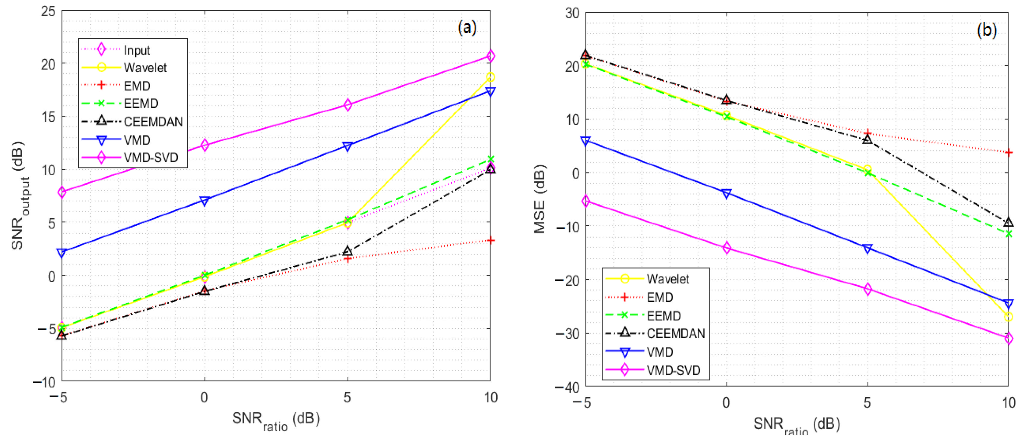
| Block | −5 dB | −4.9435 | 10.36 | −5.711 | 12.363 | −4.9089 | 10.278 | −5.7292 | 12.415 | 7.8549 | 0.5439 |
| 0 dB | −0.1372 | 3.4257 | −1.4703 | 4.6565 | 0.0014 | 3.3181 | −1.5215 | 4.7116 | 12.261 | 0.1979 | |
| 5 dB | 4.9576 | 1.0599 | 1.5734 | 2.3104 | 5.2345 | 0.9944 | 2.2105 | 1.9952 | 16.071 | 0.082 | |
| 10 dB | 18.691 | 0.0448 | 3.3386 | 1.5387 | 10.922 | 0.2684 | 9.9553 | 0.3353 | 20.682 | 0.0283 | |
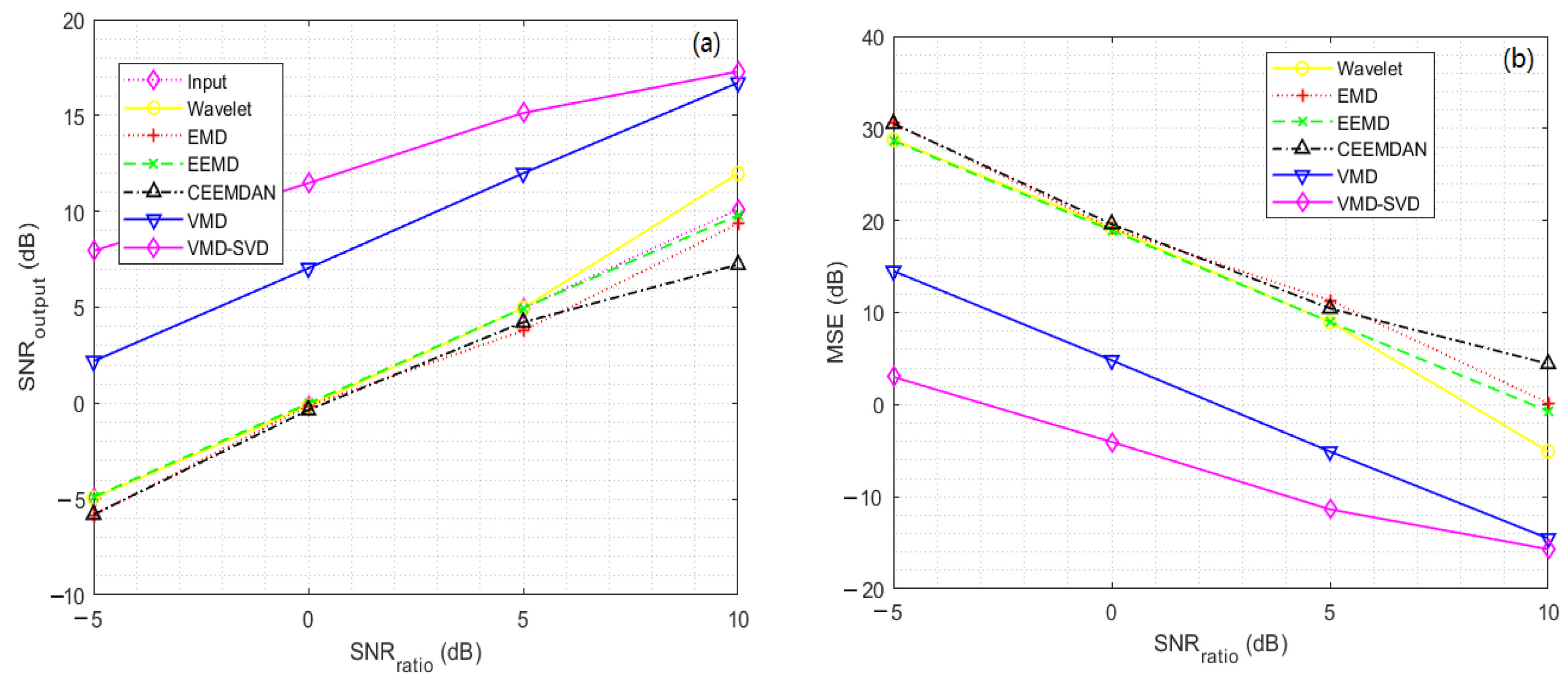
| Bump | −5 dB | −4.9435 | 27.471 | −5.843 | 33.793 | −4.8836 | 27.094 | −5.808 | 33.521 | 7.9391 | 1.4145 |
| 0 dB | −0.1372 | 9.0832 | −0.1268 | 9.0616 | −0.016 | 8.8336 | −0.3599 | 9.5612 | 11.47 | 0.627 | |
| 5 dB | 4.9576 | 2.8104 | 3.7765 | 3.6887 | 4.9525 | 2.8137 | 4.2177 | 3.3324 | 15.133 | 0.269 | |
| 10 dB | 11.98 | 0.5579 | 9.3555 | 1.0209 | 9.8018 | 0.9211 | 7.2264 | 1.668 | 17.292 | 0.164 | |
| Parameters | Parameter Index |
|---|---|
| Laser | Nd:YAG laser |
| Wavelength | 1064 nm, 532 nm, 355 nm |
| Single pulse energy (1064 mm/532 mm/355 mm) | 350 mJ/170 mJ/80 mJ |
| Impulse frequency | 1–10 Hz |
| Pulse width (1064 nm) | ≤10 ns |
| Beam diameter (1064 nm) | ~9 mm |
| Divergence angle (1064 nm) | ≤0.5 mrad |
| Telescope | Schmidt–Cassegrain type |
| Diameter | 300 mm |
| Field of view angle | 0.4 mrad |
| Horizontal angle | 0–360° |
| Pitching angle | 0–90° |
| Detection range | 100–13,000 m (Night), 100–10,000 m (Daytime) |
| Wavelet Threshold | EMD | EEMD | CEEMD | VMD-SSA-SVD | |
|---|---|---|---|---|---|
| SNR | 16.3059 | 8.4232 | 11.9542 | 16.2208 | 21.1368 |
| MSE | 5.299 × 10⁻⁷ | 1.412 × 10⁻⁶ | 3.139 × 10⁻⁷ | 2.345 × 10⁻⁷ | 7.56 × 10⁻⁸ |
| Wavelet Threshold | EMD | EEMD | CEEMD | VMD-SSA-SVD | |
|---|---|---|---|---|---|
| SNR | 17.3105 | 7.8042 | 9.9699 | 14.7930 | 22.3783 |
| MSE | 2.699 × 10⁻⁷ | 5.302 × 10⁻⁶ | 3.239 × 10⁻⁶ | 3.749 × 10⁻⁶ | 2.16 × 10⁻⁷ |
| Wavelet Threshold | EMD | EEMD | CEEMD | VMD-SSA-SVD | |
|---|---|---|---|---|---|
| SNR | 20.5950 | 8.6486 | 11.0205 | 17.5588 | 23.6226 |
| MSE | 5.285 × 10⁻⁶ | 1.161 × 10⁻⁵ | 3.904 × 10⁻⁵ | 4.235 × 10⁻⁶ | 7.23 × 10⁻⁷ |
Publisher’s Note: MDPI stays neutral with regard to jurisdictional claims in published maps and institutional affiliations. |
© 2022 by the authors. Licensee MDPI, Basel, Switzerland. This article is an open access article distributed under the terms and conditions of the Creative Commons Attribution (CC BY) license (https://creativecommons.org/licenses/by/4.0/).
Share and Cite
Li, Z.; Li, S.; Mao, J.; Li, J.; Wang, Q.; Zhang, Y. A Novel Lidar Signal-Denoising Algorithm Based on Sparrow Search Algorithm for Optimal Variational Modal Decomposition. Remote Sens. 2022, 14, 4960. https://doi.org/10.3390/rs14194960
Li Z, Li S, Mao J, Li J, Wang Q, Zhang Y. A Novel Lidar Signal-Denoising Algorithm Based on Sparrow Search Algorithm for Optimal Variational Modal Decomposition. Remote Sensing. 2022; 14(19):4960. https://doi.org/10.3390/rs14194960
Chicago/Turabian StyleLi, Zhiyuan, Shun Li, Jiandong Mao, Juan Li, Qiang Wang, and Yi Zhang. 2022. "A Novel Lidar Signal-Denoising Algorithm Based on Sparrow Search Algorithm for Optimal Variational Modal Decomposition" Remote Sensing 14, no. 19: 4960. https://doi.org/10.3390/rs14194960