A CNN Ensemble Based on a Spectral Feature Refining Module for Hyperspectral Image Classification
Abstract
1. Introduction
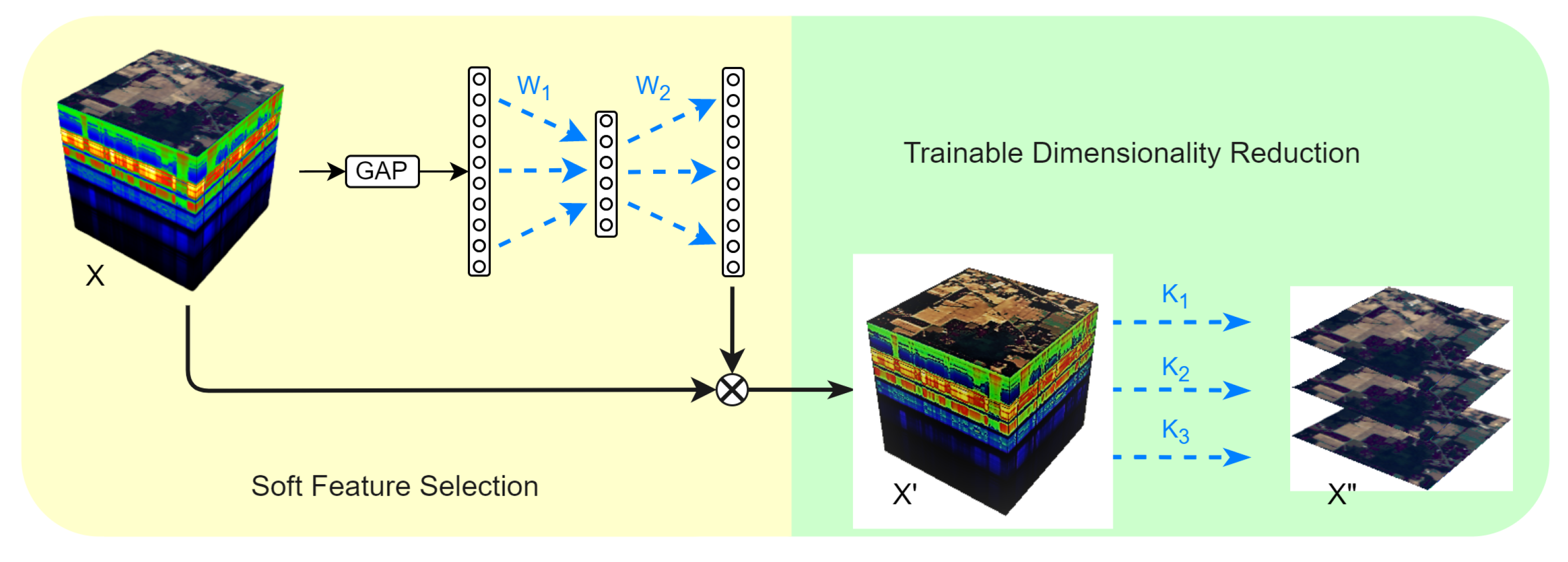
- We propose a trainable spectral feature refining module that is an effective dimensionality reduction technique for HSI classification. While the widely used projection-based dimensionality reduction techniques are usually implemented independently in the preprocessing stages of HSI classification tasks, the proposed spectral feature refining is more like an internal process of the classifier and can be optimized directly for improving the classification results.
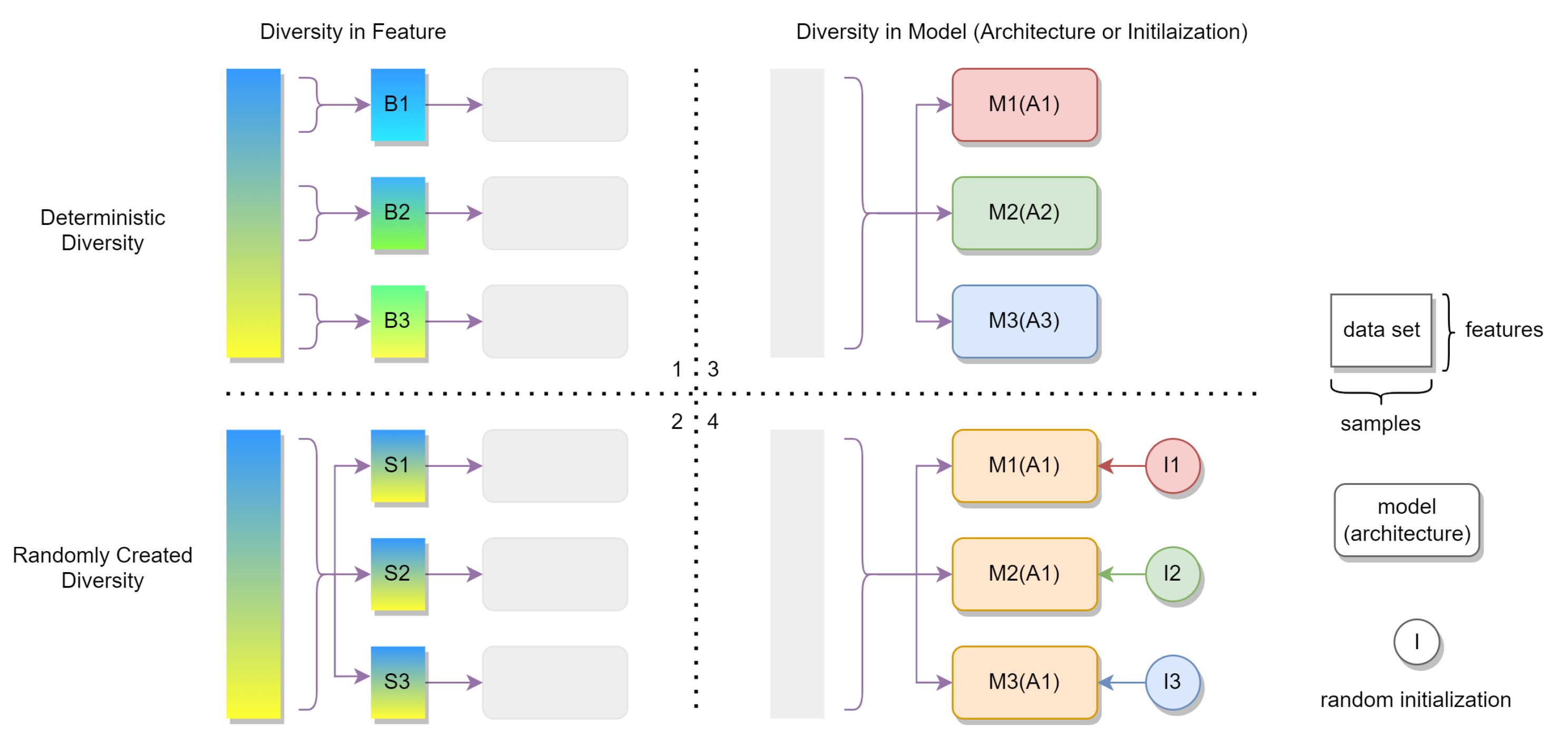
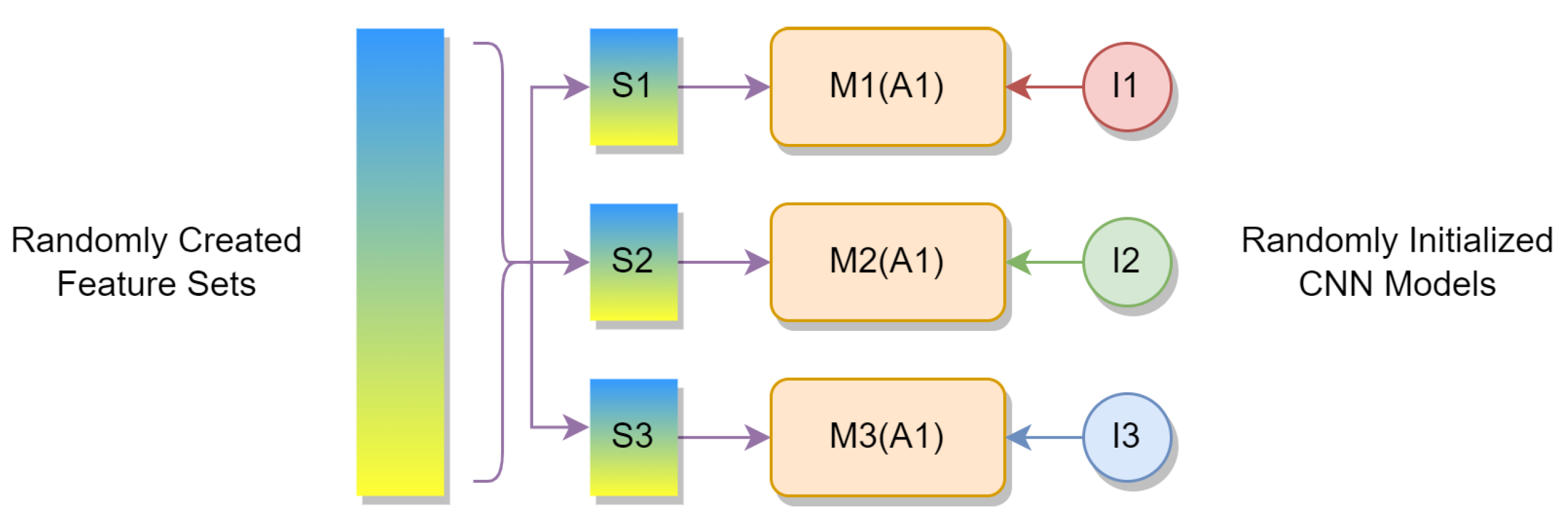
- A new ensemble learning strategy for HSI classification is established based on the proposed spectral feature refining module and the inherent randomness of CNN models. Using such a simple strategy, it is quite convenient to produce diversity among base classifiers. Without explicitly splitting the original spectral feature space, the base classifiers are automatically trained on different low dimensional spectral feature subspaces produced by the embedded spectral feature refining modules.
2. Related Works
2.1. CNN Ensembles for HSI Classification
2.2. Channel Attention
3. Proposed Method
3.1. Channel Attention-Based Spectral Feature Refining
- It is more convenient since the process of dimensionality reduction is no longer an extra preprocessing step previous to the feature extraction and classification processes.
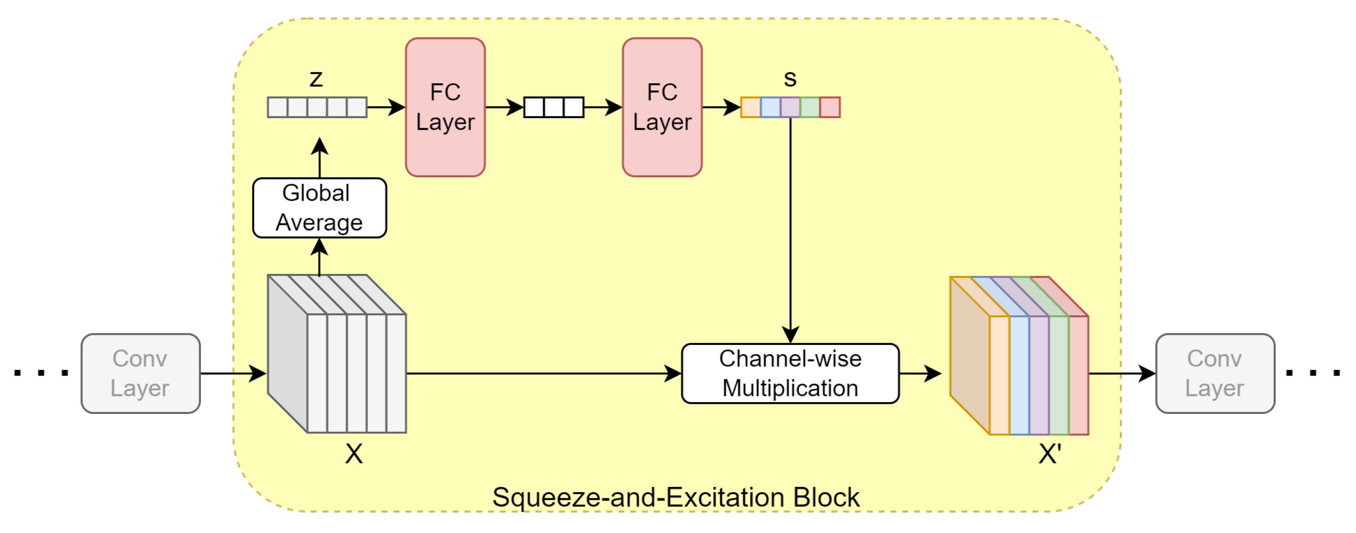
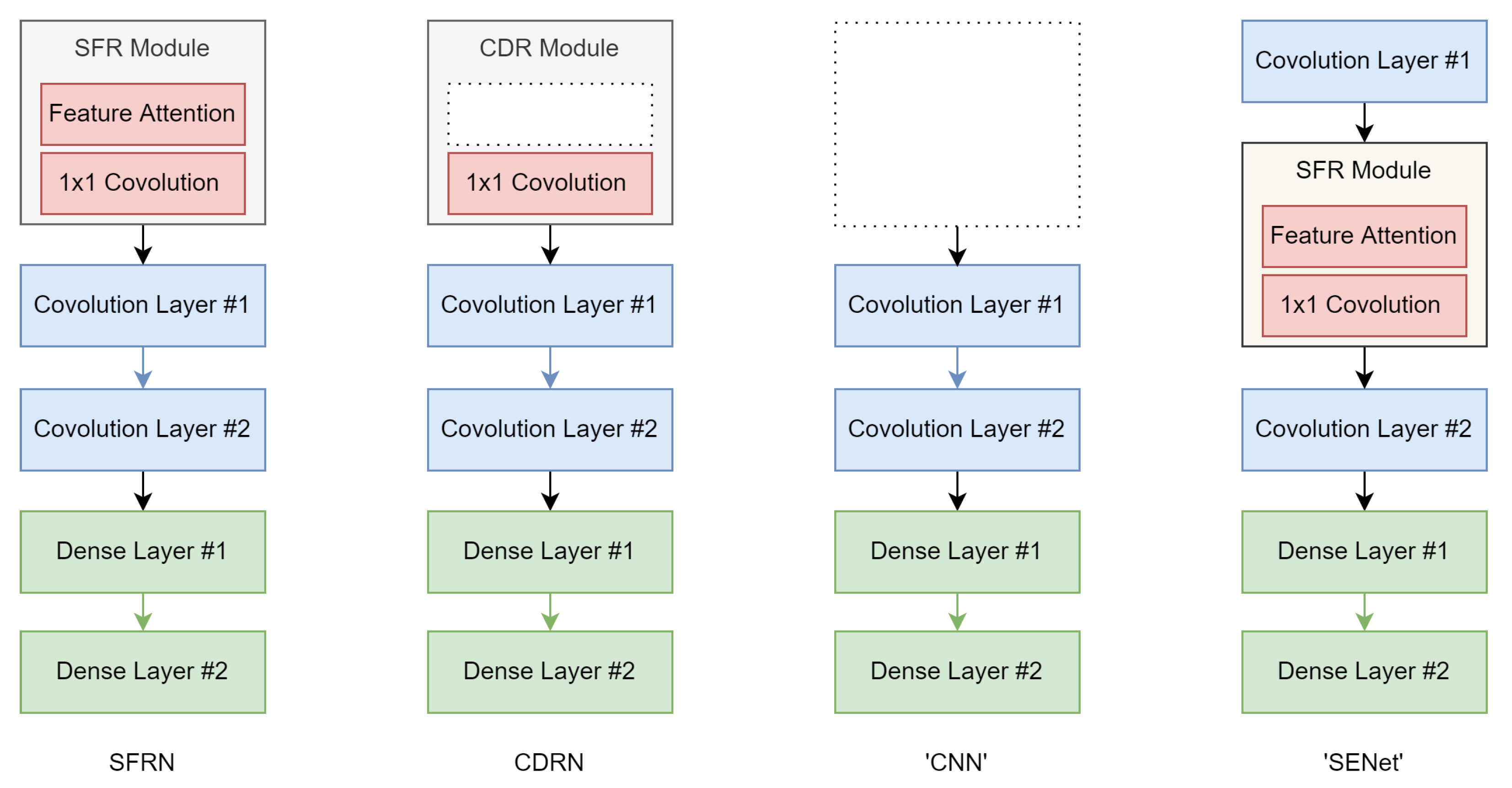
- Both the channel attention operation and the 1 × 1 convolution layer contain trainable parameters. Therefore, the spectral feature refining module can be optimized during the training stage of the SFRN model. This process not only reduces the dimensionality of HSIs, but also refines the spectral features for the classification task.
- More importantly, as in a SFRN, the training processes of the spectral feature refining part, the semantic feature extraction part and the classification part are implemented simultaneously using the same objective function. Hence, all the parts are optimized to the same direction.
3.2. SFRN Ensemble
3.3. Discussion
4. Experimental Results
4.1. Data Set Description and Experimental Setup
- The IP image was captured in 1992 by the 224-band airborne visible/infrared imaging spectrometer (AVIRIS) [44] over the Indian Pines test site in Northwestern Indiana, USA. The image contains pixels with a spatial resolution of 20 mpp. Here, 200 bands in the spectral range of 0.4–2.5 μm are selected out of the original image, then 10,249 pixels in the image are labeled and divided into 16 classes to form the data set.
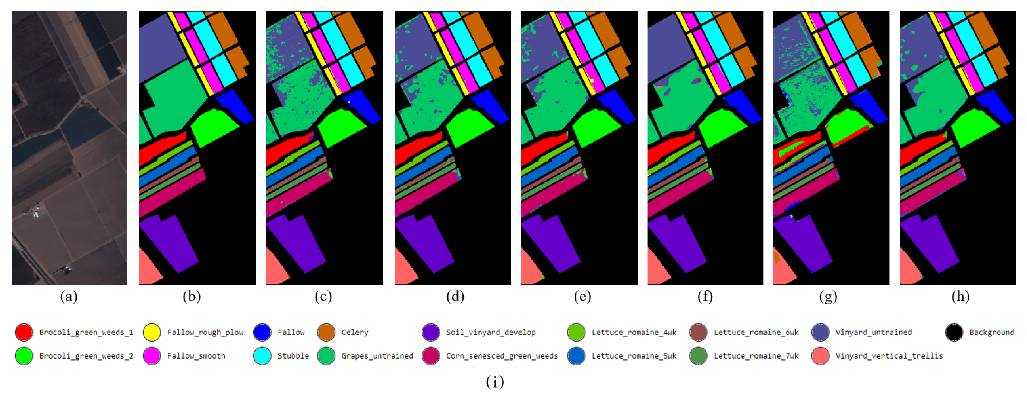
- The SA data set is another data set gathered by the AVIRIS sensor. The campaign was conducted in 1998 over the agricultural area of Salinas Valley, California. The image contains pixels with a spatial resolution of 3.7 mpp. Here, 20 bands in the original image are discarded due to water absorption and noise. The data set contains 54,129 pixels belonging to 16 different classes.
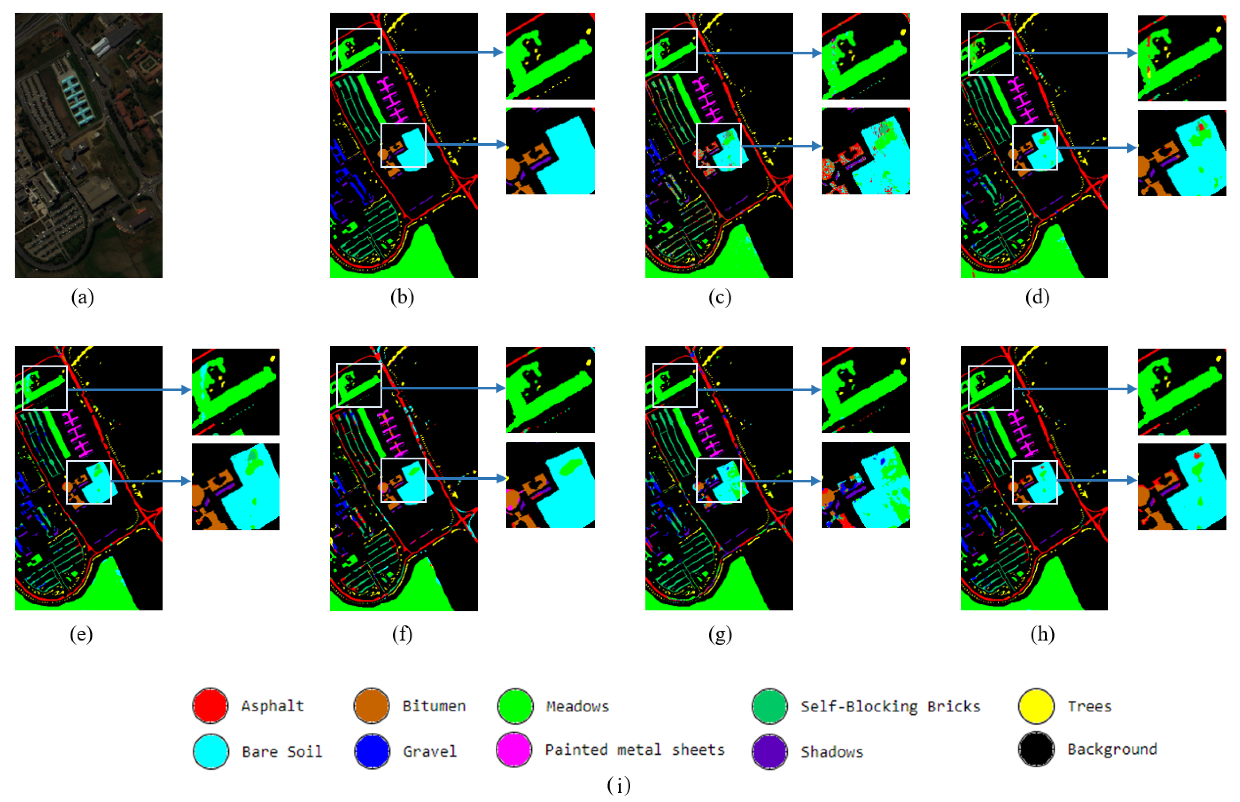
- The PU image was captured by the reflective optics system imaging spectrometer (ROSIS) [45] over the campus of the University of Pavia, in the north of Italy. The image contains pixels with a spatial resolution of 1.3 mpp. After discarding the noisy bands, 103 out of the 115 original spectral bands, covering the spectral range from 0.43 to 0.86 μm, are kept to form the data set. It contains 42,776 pixels which can be categorized as nine different classes that belong to an urban environment with multiple solid structures, natural objects and shadows.
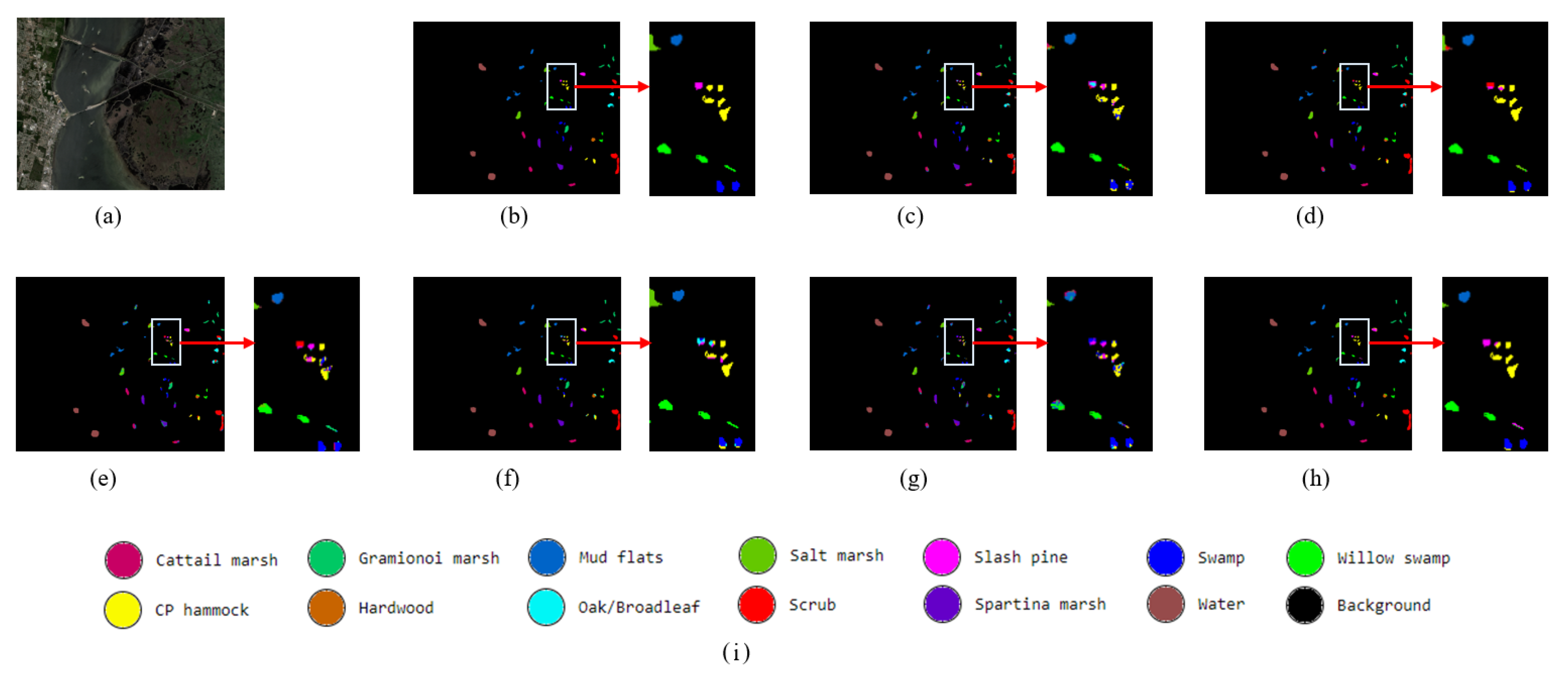
- The KSC image was also captured by the AVIRIS sensor. The campaign was conducted in 1996 over the neighborhood of the Kennedy Space Center in Florida, USA. The image contains pixels with a spatial resolution of 18 mpp. Only 176 spectral bands ranging from 0.4 to 2.5 μm are kept in the data set, which contains 5211 labeled pixels belonging to 13 different land cover classes.
4.2. Spectral Redundancy and Dimensionality Reduction
4.3. Classification Performance
4.4. Comparisons with Other Ensembles
4.5. Ablation Analysis
5. Conclusions
Author Contributions
Funding
Data Availability Statement
Acknowledgments
Conflicts of Interest
Abbreviations
| CDR | Convolution-based dimensionality reduction |
| SFR | Spectral feature refining, which is a module for dimensionality reduction |
| SFRN | Spectral feature refining network, a CNN equipped with a SFR module |
| SFRN-E | Spectral feature refining network ensemble, an ensemble of multiple SFRNs |
References
- Camps-Valls, G.; Tuia, D.; Bruzzone, L.; Benediktsson, J.A. Advances in Hyperspectral Image Classification: Earth Monitoring with Statistical Learning Methods. IEEE Signal Process. Mag. 2014, 31, 45–54. [Google Scholar] [CrossRef]
- Tong, Q.; Xue, Y.; Zhang, L. Progress in Hyperspectral Remote Sensing Science and Technology in China Over the Past Three Decades. IEEE J. Sel. Top. Appl. Earth Obs. Remote Sens. 2014, 7, 70–91. [Google Scholar] [CrossRef]
- Hughes, G. On the mean accuracy of statistical pattern recognizers. IEEE Trans. Inf. Theory 1968, 14, 55–63. [Google Scholar] [CrossRef]
- Xia, J.; Liao, W.; Chanussot, J.; Du, P.; Song, G.; Philips, W. Improving random forest with ensemble of features and semisupervised feature extraction. IEEE Geosci. Remote Sens. Lett. 2015, 12, 1471–1475. [Google Scholar] [CrossRef]
- Falco, N.; Benediktsson, J.A.; Bruzzone, L. Spectral and spatial classification of hyperspectral images based on ICA and reduced morphological attribute profiles. IEEE Trans. Geosci. Remote Sens. 2015, 53, 6223–6240. [Google Scholar] [CrossRef]
- Shi, G.; Huang, H.; Liu, J.; Li, Z.; Wang, L. Spatial-spectral multiple manifold discriminant analysis for dimensionality reduction of hyperspectral imagery. Remote Sens. 2019, 11, 2414. [Google Scholar] [CrossRef]
- Shah, C.; Du, Q. Spatial-Aware Collaboration-Competition Preserving Graph Embedding for Hyperspectral Image Classification. IEEE Geosci. Remote Sens. Lett. 2022, 19, 1–5. [Google Scholar] [CrossRef]
- Paoletti, M.E.; Haut, J.M.; Plaza, J.; Plaza, A. Deep learning classifiers for hyperspectral imaging: A review. ISPRS J. Photogramm. Remote Sens. 2019, 158, 279–317. [Google Scholar] [CrossRef]
- Li, S.; Song, W.; Fang, L.; Chen, Y.; Ghamisi, P.; Benediktsson, J.A. Deep learning for hyperspectral image classification: An overview. IEEE Trans. Geosci. Remote Sens. 2019, 57, 1–20. [Google Scholar] [CrossRef]
- Audebert, N.; Le Saux, B.; Lefèvre, S. Deep learning for classification of hyperspectral data: A comparative review. IEEE Geosci. Remote Sens. Mag. 2019, 17, 159–173. [Google Scholar] [CrossRef]
- Lee, H.; Kwon, H. Going deeper with contextual CNN for hyperspectral image classification. IEEE Trans. Image Process. 2017, 26, 4843–4855. [Google Scholar] [CrossRef] [PubMed]
- Zhang, M.; Li, W.; Du, Q. Diverse region-based CNN for hyperspectral image classification. IEEE Trans. Image Process. 2018, 27, 2623–2634. [Google Scholar] [CrossRef] [PubMed]
- Hao, S.; Wang, W.; Ye, Y.; Nie, T.; Bruzzone, L. Two-stream deep architecture for hyperspectral image classification. IEEE Trans. Geosci. Remote Sens. 2018, 56, 2349–2361. [Google Scholar] [CrossRef]
- Xu, Y.; Zhang, L.; Du, B.; Zhang, F. Spectral-spatial unified networks for hyperspectral image classification. IEEE Trans. Geosci. Remote Sens. 2018, 56, 5893–5909. [Google Scholar] [CrossRef]
- Ma, W.; Yang, Q.; Wu, Y.; Zhao, W.; Zhang, X. Double-branch multi-attention mechanism network for hyperspectral image classification. Remote Sens. 2019, 11, 1307. [Google Scholar] [CrossRef]
- Roy, S.K.; Manna, S.; Song, T.; Bruzzone, L. Attention-based adaptive spectral-spatial kernel ResNet for hyperspectral image classification. IEEE Trans. Geosci. Remote Sens. 2020, 59, 1–13. [Google Scholar] [CrossRef]
- Hong, D.; Han, Z.; Yao, J.; Gao, L.; Zhang, B.; Plaza, A.; Chanussot, J. SpectralFormer: Rethinking Hyperspectral Image Classification with Transformers. IEEE Trans. Geosci. Remote Sens. 2022, 60, 1–5. [Google Scholar] [CrossRef]
- Zhong, Z.; Li, J.; Luo, Z.; Chapman, M. Spectral-spatial residual network for hyperspectral image classification: A 3D deep learning framework. IEEE Trans. Geosci. Remote Sens. 2018, 56, 847–858. [Google Scholar] [CrossRef]
- Roy, S.K.; Krishna, G.; Dubey, S.R.; Chaudhuri, B.B. HybridSN: Exploring 3D-2D CNN feature hierarchy for hyperspectral image classification. IEEE Geosci. Remote Sens. Lett. 2019, 17, 1–5. [Google Scholar] [CrossRef]
- Xu, H.; Yao, W.; Cheng, L.; Li, B. Multiple spectral resolution 3D convolutional neural network for hyperspectral image classification. Remote Sens. 2021, 13, 1248. [Google Scholar] [CrossRef]
- Chang, Y.L.; Tan, T.H.; Lee, W.H.; Chang, L.; Chen, Y.N.; Fan, K.C.; Alkhaleefah, M. Consolidated Convolutional Neural Network for Hyperspectral Image Classification. Remote Sens. 2022, 14, 1571. [Google Scholar] [CrossRef]
- Chen, Y.; Jiang, H.; Li, C.; Jia, X.; Ghamisi, P. Deep feature extraction and classification of hyperspectral images based on convolutional neural networks. IEEE Trans. Geosci. Remote Sens. 2016, 54, 6232–6251. [Google Scholar] [CrossRef]
- Zhang, Y.; Huynh, C.P.; Ngan, K.N. Feature fusion with predictive weighting for spectral image classification and segmentation. IEEE Trans. Geosci. Remote Sens. 2019, 57, 1–16. [Google Scholar] [CrossRef]
- Feng, J.; Yu, H.; Wang, L.; Cao, X.; Zhang, X.; Jiao, L. Classification of hyperspectral images based on multiclass spatial-spectral generative adversarial networks. IEEE Trans. Geosci. Remote Sens. 2019, 57, 5329–5343. [Google Scholar] [CrossRef]
- Santara, A.; Mani, K.; Hatwar, P.; Singh, A.; Garg, A.; Padia, K.; Mitra, P. Bass net: Band-adaptive spectral-spatial feature learning neural network for hyperspectral image classification. IEEE Trans. Geosci. Remote Sens. 2017, 55, 5293–5301. [Google Scholar] [CrossRef]
- Chen, Y.; Wang, Y.; Gu, Y.; He, X.; Ghamisi, P.; Jia, X. Deep learning ensemble for hyperspectral image classification. IEEE J. Sel. Top. Appl. Earth Obs. Remote Sens. 2019, 12, 1882–1897. [Google Scholar] [CrossRef]
- He, X.; Chen, Y. Transferring CNN ensemble for hyperspectral image classification. IEEE Geosci. Remote Sens. Lett. 2021, 18, 1–5. [Google Scholar] [CrossRef]
- Pan, S.J.; Yang, Q. A Survey on Transfer Learning. IEEE Trans. Knowl. Data Eng. 2010, 22, 1345–1359. [Google Scholar] [CrossRef]
- Russakovsky, O.; Deng, J.; Su, H.; Krause, J.; Satheesh, S.; Ma, S.; Huang, Z.; Karpathy, A.; Khosla, A.; Bernstein, M.; et al. ImageNet Large Scale Visual Recognition Challenge. Int. J. Comput. Vis. 2015, 115, 211–252. [Google Scholar] [CrossRef]
- Nalepa, J.; Myller, M.; Tulczyjew, L.; Kawulok, M. Deep Ensembles for Hyperspectral Image Data Classification and Unmixing. Remote Sens. 2021, 13, 4133. [Google Scholar] [CrossRef]
- Lv, Q.; Feng, W.; Quan, Y.; Dauphin, G.; Gao, L.; Xing, M. Enhanced-Random-Feature-Subspace-Based Ensemble CNN for the Imbalanced Hyperspectral Image Classification. IEEE J. Sel. Top. Appl. Earth Obs. Remote Sens. 2021, 14, 3988–3999. [Google Scholar] [CrossRef]
- Manian, V.; Alfaro-Mejía, E.; Tokars, R.P. Hyperspectral Image Labeling and Classification Using an Ensemble Semi-Supervised Machine Learning Approach. Sensors 2022, 22, 1623. [Google Scholar] [CrossRef] [PubMed]
- Liu, B.; Gao, K.; Yu, A.; Ding, L.; Qiu, C.; Li, J. ES2FL: Ensemble Self-Supervised Feature Learning for Small Sample Classification of Hyperspectral Images. Remote Sens. 2022, 14, 4236. [Google Scholar] [CrossRef]
- Brown, G.; Wyatt, J.; Harris, R.; Yao, X. Diversity creation methods: A survey and categorisation. Inf. Fusion 2005, 6, 5–20. [Google Scholar] [CrossRef]
- Minetto, R.; Segundo, M.P.; Sarkar, S. Hydra: An ensemble of convolutional neural networks for geospatial land classification. IEEE Trans. Geosci. Remote Sens. 2019, 57, 1–12. [Google Scholar] [CrossRef]
- He, K.; Zhang, X.; Ren, S.; Sun, J. Deep Residual Learning for Image Recognition. In Proceedings of the IEEE Conference on Computer Vision and Pattern Recognition (CVPR), Las Vegas, NV, USA, 27–30 June 2016. [Google Scholar]
- Huang, G.; Liu, Z.; van der Maaten, L.; Weinberger, K.Q. Densely connected convolutional networks. In Proceedings of the IEEE/CVF Conference on Computer Vision and Pattern Recognition (CVPR), Honolulu, HI, USA, 21–26 July 2017; pp. 4700–4708. [Google Scholar]
- Zhou, Z.; Wu, J.; Tang, W. Ensembling neural networks: Many could be better than all. Artif. Intell. 2002, 137, 239–263. [Google Scholar] [CrossRef]
- Mei, X.; Pan, E.; Ma, Y.; Dai, X.; Huang, J.; Fan, F.; Du, Q.; Zheng, H.; Ma, J. Spectral-spatial attention networks for hyperspectral image classification. Remote Sens. 2019, 11, 963. [Google Scholar] [CrossRef]
- Sun, H.; Zheng, X.; Lu, X.; Wu, S. Spectral-spatial attention network for hyperspectral image classification. IEEE Trans. Geosci. Remote Sens. 2020, 58, 3232–3245. [Google Scholar] [CrossRef]
- Hu, J.; Shen, L.; Sun, G. Squeeze and excitation networks. In Proceedings of the IEEE/CVF Conference on Computer Vision and Pattern Recognition (CVPR), Salt Lake City, UT, USA, 18–23 June 2018. [Google Scholar]
- Nair, V.; Hinton, G.E. Rectified linear units improve restricted boltzmann machines. In Proceedings of the International Conference on Machine Learning (ICML), Haifa, Israel, 21–24 June 2010; pp. 807–814. [Google Scholar] [CrossRef]
- Glorot, X.; Bordes, A.; Bengio, Y. Deep sparse rectifier neural networks. In Proceedings of the 14th International Conference on Artificial Intelligence and Statistics (AISTATS), Fort Lauderdale, FL, USA, 11–13 April 2011; pp. 315–323. [Google Scholar]
- Green, R.O.; Eastwood, M.L.; Sarture, C.M.; Chrien, T.G.; Aronsson, M.; Chippendale, B.J.; Faust, J.A.; Pavri, B.E.; Chovit, C.J.; Solis, M.; et al. Imaging Spectroscopy and the Airborne Visible/Infrared Imaging Spectrometer (AVIRIS). Remote Sens. Environ. 1998, 65, 227–248. [Google Scholar] [CrossRef]
- Kunkel, B.; Blechinger, F.; Lutz, R.; Doerffer, R.; van der Piepen, H.; Schroder, M. ROSIS (Reflective Optics System Imaging Spectrometer)—A candidate instrument for polar platform missions. In Proceedings of the Optoelectronic Technologies for Remote Sensing from Space, Cannes, France, 17–20 November 1987; Bowyer, C.S., Seeley, J.S., Eds.; International Society for Optics and Photonics, SPIE: Bellingham, WA, USA, 1988; Volume 0868, pp. 134–141. [Google Scholar] [CrossRef]
- Chakraborty, T.; Trehan, U. SpectralNET: Exploring Spatial-Spectral WaveletCNN for Hyperspectral Image Classification. arXiv 2021, arXiv:2104.00341. [Google Scholar]



| Label | Class Name | Training/Test | CDCNN | SSRN | DBMA | HybridSN | SpectralNet | SFRN-E |
|---|---|---|---|---|---|---|---|---|
| 1 | Alfalfa | 2/44 | 42.72 | 46.15 | 68.24 | 88.61 | 56.82 | 82.67 |
| 2 | Corn-notill | 25/1403 | 58.82 | 71.83 | 73.58 | 66.92 | 65.72 | 89.06 |
| 3 | Corn-mintill | 13/817 | 46.15 | 77.43 | 70.44 | 56.60 | 69.25 | 65.19 |
| 4 | Corn | 3/234 | 29.59 | 25.19 | 52.70 | 38.62 | 25.74 | 64.76 |
| 5 | Grass-pasture | 7/476 | 89.15 | 80.87 | 80.92 | 75.83 | 64.39 | 84.67 |
| 6 | Grass-trees | 12/718 | 94.25 | 94.15 | 88.68 | 93.99 | 81.46 | 87.88 |
| 7 | Grass-pasture-mowed | 1/27 | 9.76 | 0.00 | 25.00 | 66.67 | 46.67 | 75.00 |
| 8 | Hay-windrowed | 14/464 | 94.14 | 97.71 | 96.30 | 75.51 | 99.46 | 97.83 |
| 9 | Oats | 1/19 | 12.24 | 0.00 | 0.00 | 58.18 | 25.00 | 27.50 |
| 10 | Soybean-notill | 25/947 | 68.74 | 78.04 | 80.29 | 75.19 | 74.90 | 87.67 |
| 11 | Soybean-mintill | 48/2407 | 75.75 | 85.08 | 86.76 | 86.00 | 79.05 | 94.62 |
| 12 | Soybean-clean | 11/582 | 44.89 | 52.61 | 71.08 | 53.75 | 60.06 | 75.74 |
| 13 | Wheat | 4/201 | 82.06 | 86.44 | 85.09 | 81.82 | 96.68 | 96.16 |
| 14 | Woods | 28/1237 | 92.49 | 91.36 | 94.77 | 96.14 | 90.81 | 97.37 |
| 15 | Buildings-Grass-Trees-Drives | 5/381 | 66.67 | 24.35 | 53.99 | 54.77 | 51.50 | 52.69 |
| 16 | Stone-Steel-Towers | 1/92 | 70.27 | 55.93 | 17.82 | 42.11 | 35.77 | 62.94 |
| OA(%) | 72.03 ± 1.29 | 78.48 ± 0.96 | 80.86 ± 1.80 | 77.07 ± 2.51 | 75.07 ± 2.03 | 86.39 ± 0.92 | ||
| AA(%) | 62.88 ± 1.71 | 57.42 ± 2.98 | 64.70 ± 2.74 | 70.30 ± 3.66 | 61.07 ± 3.24 | 75.87 ± 2.60 | ||
| Kappa × 100 | 68.03 ± 1.49 | 75.30 ± 1.12 | 78.10 ± 2.06 | 73.83 ± 2.84 | 71.05 ± 2.31 | 84.44 ± 1.03 | ||
| Label | Class Name | Training/Test | CDCNN | SSRN | DBMA | HybridSN | SpectralNet | SFRN-E |
|---|---|---|---|---|---|---|---|---|
| 1 | Brocoli_green_weeds_1 | 7/2002 | 99.98 | 100.00 | 98.84 | 99.63 | 76.06 | 98.50 |
| 2 | Brocoli_green_weeds_2 | 14/3712 | 96.80 | 99.93 | 99.92 | 99.72 | 85.63 | 99.68 |
| 3 | Fallow | 7/1969 | 99.46 | 95.57 | 96.63 | 91.48 | 91.97 | 98.41 |
| 4 | Fallow_rough_plow | 5/1389 | 92.84 | 98.55 | 96.58 | 95.59 | 95.96 | 93.63 |
| 5 | Fallow_smooth | 10/2668 | 95.20 | 98.39 | 95.83 | 96.49 | 97.16 | 96.36 |
| 6 | Stubble | 15/3944 | 99.23 | 100.00 | 99.23 | 96.34 | 99.51 | 99.39 |
| 7 | Celery | 13/3566 | 99.92 | 99.87 | 99.86 | 99.87 | 94.49 | 98.87 |
| 8 | Grapes_untrained | 42/11,229 | 83.50 | 88.04 | 92.06 | 94.06 | 82.08 | 92.81 |
| 9 | Soil_vinyard_develop | 23/6180 | 99.19 | 99.72 | 99.57 | 100.00 | 98.66 | 99.51 |
| 10 | Corn_senesced_green_ weeds | 12/3266 | 92.70 | 94.12 | 93.56 | 98.00 | 92.27 | 95.92 |
| 11 | Lettuce_romaine_4wk | 4/1064 | 93.53 | 96.61 | 92.26 | 79.50 | 74.97 | 97.38 |
| 12 | Lettuce_romaine_5wk | 7/1920 | 96.75 | 99.12 | 99.46 | 100.00 | 91.57 | 95.29 |
| 13 | Lettuce_romaine_6wk | 3/913 | 83.38 | 98.85 | 99.51 | 91.91 | 93.38 | 92.92 |
| 14 | Lettuce_romaine_7wk | 4/1066 | 90.86 | 96.44 | 94.42 | 82.45 | 97.20 | 94.42 |
| 15 | Vinyard_untrained | 27/7241 | 76.69 | 78.13 | 90.00 | 92.05 | 76.31 | 89.89 |
| 16 | Vinyard_vertical_trellis | 7/1800 | 98.24 | 99.20 | 98.28 | 80.57 | 92.08 | 99.02 |
| OA(%) | 91.40 ± 0.48 | 93.82 ± 0.51 | 95.70 ± 0.37 | 95.15 ± 0.92 | 88.42 ± 1.47 | 95.75 ± 0.27 | ||
| AA(%) | 94.09 ± 0.75 | 96.41 ± 0.90 | 97.31 ± 0.39 | 93.69 ± 1.63 | 89.98 ± 1.35 | 96.59 ± 0.44 | ||
| Kappa × 100 | 90.44 ± 0.54 | 93.11 ± 0.58 | 95.22 ± 0.42 | 94.61 ± 1.02 | 87.13 ± 1.64 | 95.27 ± 0.29 | ||
| Label | Class Name | Training/ Test | CDCNN | SSRN | DBMA | HybridSN | SpectralNet | SFRN-E |
|---|---|---|---|---|---|---|---|---|
| 1 | Asphalt | 31/6600 | 88.86 | 91.80 | 95.28 | 85.37 | 85.94 | 91.39 |
| 2 | Meadows | 87/18,562 | 96.53 | 97.53 | 97.10 | 97.69 | 92.32 | 98.70 |
| 3 | Gravel | 10/2089 | 64.82 | 75.81 | 76.92 | 76.90 | 59.11 | 79.62 |
| 4 | Trees | 14/3050 | 92.51 | 94.04 | 94.35 | 68.37 | 89.11 | 93.70 |
| 5 | Painted metal sheets | 6/1339 | 99.96 | 99.87 | 99.32 | 88.40 | 95.64 | 99.51 |
| 6 | Bare Soil | 24/5005 | 86.51 | 91.63 | 90.16 | 92.83 | 79.42 | 94.93 |
| 7 | Bitumen | 6/1324 | 74.95 | 91.74 | 91.95 | 78.20 | 66.00 | 88.84 |
| 8 | Self-Blocking Bricks | 17/3665 | 75.49 | 84.00 | 81.86 | 71.76 | 82.03 | 78.30 |
| 9 | Shadows | 5/942 | 78.65 | 91.37 | 94.42 | 53.26 | 70.27 | 90.47 |
| OA(%) | 89.70 ± 0.76 | 93.25 ± 0.89 | 93.33 ± 0.77 | 88.25 ± 3.42 | 86.36 ± 2.04 | 93.58 ± 0.89 | ||
| AA(%) | 83.77 ± 1.90 | 90.35 ± 1.37 | 91.44 ± 1.28 | 79.16 ± 7.83 | 77.15 ± 2.28 | 89.01 ± 1.26 | ||
| Kappa × 100 | 86.27 ± 0.98 | 91.05 ± 1.16 | 91.17 ± 1.02 | 84.31 ± 4.68 | 81.51 ± 2.56 | 91.46 ± 1.18 | ||
| Label | Class Name | Training/Test | CDCNN | SSRN | DBMA | HybridSN | SpectralNet | SFRN-E |
|---|---|---|---|---|---|---|---|---|
| 1 | Scrub | 29/732 | 85.20 | 88.54 | 84.00 | 96.85 | 89.27 | 100.00 |
| 2 | Willow swamp | 9/234 | 78.74 | 77.29 | 68.78 | 79.53 | 67.02 | 91.03 |
| 3 | CP hammock | 10/246 | 86.56 | 93.14 | 84.94 | 93.75 | 59.66 | 97.07 |
| 4 | Slash pine | 10/242 | 64.79 | 80.72 | 71.36 | 78.44 | 42.86 | 90.42 |
| 5 | Oak/Broadleaf | 6/155 | 61.86 | 75.86 | 65.55 | 76.87 | 73.97 | 88.26 |
| 6 | Hardwood | 9/220 | 61.21 | 74.01 | 66.81 | 89.50 | 69.72 | 100.00 |
| 7 | Swamp | 4/101 | 64.76 | 65.22 | 80.46 | 79.56 | 87.83 | 88.40 |
| 8 | Gramionoi marsh | 17/414 | 95.48 | 93.51 | 77.83 | 97.62 | 65.59 | 97.30 |
| 9 | Spartina marsh | 20/500 | 90.96 | 93.30 | 86.12 | 96.59 | 80.47 | 99.70 |
| 10 | Cattail marsh | 15/389 | 89.45 | 91.50 | 84.38 | 99.62 | 75.28 | 100.00 |
| 11 | Salt marsh | 16/403 | 75.19 | 79.20 | 72.29 | 86.97 | 91.18 | 100.00 |
| 12 | Mud flats | 19/484 | 89.16 | 88.66 | 80.82 | 94.55 | 77.79 | 100.00 |
| 13 | Water | 36/891 | 95.91 | 95.02 | 96.74 | 96.01 | 96.42 | 100.00 |
| OA(%) | 85.05 ± 0.99 | 88.15 ± 1.40 | 82.18 ± 2.00 | 92.96 ± 1.43 | 79.82 ± 2.01 | 98.14 ± 0.18 | ||
| AA(%) | 80.18 ± 0.92 | 81.67 ± 2.25 | 76.95 ± 2.44 | 88.49 ± 1.59 | 74.92 ± 2.53 | 95.54 ± 0.47 | ||
| Kappa × 100 | 83.36 ± 01.09 | 86.73 ± 1.61 | 80.10 ± 2.23 | 92.14 ± 1.62 | 77.53 ± 2.25 | 97.93 ± 0.20 | ||
| Data Sets | Metrics | SVM-E | CNN-E | TCNN-E | TCNN-E | SFRN-E |
|---|---|---|---|---|---|---|
| (with Label Smoothing) | (with Label Smoothing) | |||||
| OA(%) | 81.61 ± 1.47 | 88.62 ± 0.36 | 90.17 ± 2.16 | 91.88 ± 1.13 | 91.62 ± 0.45 | |
| IP | AA(%) | 57.51 ± 4.24 | 66.55 ± 3.49 | 71.53 ± 5.83 | 77.37 ± 4.04 | 80.02 ± 0.91 |
| Kappa × 100 | 77.62 ± 1.83 | 86.30 ± 0.43 | 88.21 ± 2.60 | 90.28 ± 1.34 | 90.43 ± 0.51 | |
| OA(%) | - | 84.02 | 87.94 | 89.62 | 94.18 ± 0.35 | |
| PU | AA(%) | - | 83.71 | 82.98 | 85.14 | 89.34 ± 0.58 |
| Kappa × 100 | - | 84.76 | 84.21 | 86.51 | 92.25 ± 0.47 | |
| OA(%) | 91.57 ± 2.47 | 96.85 ± 0.69 | 97.29 ± 1.51 | 99.27 ± 0.36 | 99.28 ± 0.30 | |
| KSC | AA(%) | 87.10 ± 3.43 | 95.90 ± 0.94 | 96.06 ± 2.14 | 98.87 ± 0.64 | 98.33 ± 0.67 |
| Kappa × 100 | 90.60 ± 2.76 | 96.50 ± 0.76 | 96.98 ± 1.68 | 99.19 ± 0.41 | 99.20 ± 0.33 |
| Models | CDCNN | SSRN | DBMA | HybridSN | SpectralNet | CNN-E | TCNN-E | SFRN-E |
|---|---|---|---|---|---|---|---|---|
| Parameter Amount | 0.303 M | 0.310 M | 0.06 M | 6.781 M | 6.802 M | 1.118 M | 34.822 M | 2.721 M |
| Data Sets | Metrics | “CNN” Ensemble | CDRN Ensemble | “SENet” Ensemble | SFRN Ensemble |
|---|---|---|---|---|---|
| OA(%) | 73.31 ± 0.25 | 88.33 ± 0.94 | 90.75 ± 0.24 | 91.62 ± 0.45 | |
| IP | AA(%) | 65.00 ± 0.35 | 72.74 ± 2.61 | 78.41 ± 0.65 | 80.02 ± 0.91 |
| Kappa × 100 | 69.34 ± 0.28 | 86.60 ± 1.09 | 89.83 ± 0.28 | 90.43 ± 0.51 | |
| OA(%) | 90.26 ± 0.15 | 94.47 ± 0.33 | 95.06 ± 0.09 | 95.46 ± 0.18 | |
| SA | AA(%) | 92.65 ± 0.18 | 95.83 ± 0.56 | 97.35 ± 0.23 | 97.02 ± 0.42 |
| Kappa × 100 | 89.15 ± 0.17 | 93.84 ± 0.37 | 94.50 ± 0.10 | 94.95 ± 0.19 | |
| OA(%) | 89.77 ± 0.14 | 90.46 ± 0.38 | 92.78 ± 0.37 | 94.18 ± 0.35 | |
| PU | AA(%) | 86.89 ± 0.22 | 83.65 ± 0.93 | 88.55 ± 0.99 | 89.34 ± 0.58 |
| Kappa × 100 | 86.30 ± 0.19 | 87.23 ± 0.52 | 90.35 ± 0.51 | 92.25 ± 0.47 | |
| OA(%) | 59.07 ± 0.47 | 97.31 ± 0.35 | 99.06 ± 0.14 | 99.28 ± 0.30 | |
| KSC | AA(%) | 46.54 ± 0.91 | 93.65 ± 0.76 | 97.32 ± 0.42 | 98.33 ± 0.67 |
| Kappa × 100 | 54.20 ± 0.55 | 97.00 ± 0.39 | 98.96 ± 0.16 | 99.20 ± 0.33 |
Publisher’s Note: MDPI stays neutral with regard to jurisdictional claims in published maps and institutional affiliations. |
© 2022 by the authors. Licensee MDPI, Basel, Switzerland. This article is an open access article distributed under the terms and conditions of the Creative Commons Attribution (CC BY) license (https://creativecommons.org/licenses/by/4.0/).
Share and Cite
Yao, W.; Lian, C.; Bruzzone, L. A CNN Ensemble Based on a Spectral Feature Refining Module for Hyperspectral Image Classification. Remote Sens. 2022, 14, 4982. https://doi.org/10.3390/rs14194982
Yao W, Lian C, Bruzzone L. A CNN Ensemble Based on a Spectral Feature Refining Module for Hyperspectral Image Classification. Remote Sensing. 2022; 14(19):4982. https://doi.org/10.3390/rs14194982
Chicago/Turabian StyleYao, Wei, Cheng Lian, and Lorenzo Bruzzone. 2022. "A CNN Ensemble Based on a Spectral Feature Refining Module for Hyperspectral Image Classification" Remote Sensing 14, no. 19: 4982. https://doi.org/10.3390/rs14194982
APA StyleYao, W., Lian, C., & Bruzzone, L. (2022). A CNN Ensemble Based on a Spectral Feature Refining Module for Hyperspectral Image Classification. Remote Sensing, 14(19), 4982. https://doi.org/10.3390/rs14194982


