Abstract
The eddy covariance (EC) technique has been widely used as a micrometeorological tool to measure carbon, water and energy exchanges. When utilizing the EC measurements, it is critical to be aware of the long-term information on source areas. In China, large-scale forest plantations have become a dominant driver of greening and carbon sinks on the planet. However, the spatial representativeness of EC measurements on forest plantations is still not well understood. Here, an EC flux site of a coniferous plantation mixed with cropland in a subtropical monsoon climate was selected to evaluate the spatial representativeness of the two approaches. One is the fraction of target vegetation type (FTVT), which was used to detect to what degree the flux is related to the target vegetation. The other is the sensor location bias calculated from the enhanced vegetation index (EVI), which was used to detect to what spatial extent the flux can be upscaled. The results showed that the monthly footprint climatologies changed intensely throughout the year. The source area is biased toward the southeast in summer and northwest in winter. The study area was mainly a composite of coniferous plantations (70.08%) and double-cropped rice (27.83%). The double-cropped rice, with a higher seasonal variation of EVI than the coniferous plantation, was mainly distributed in the eastern areas of the study site. As a result of spatial heterogeneity and footprint variation, the FTVT was 0.89 when the wind direction was southwest; however, this reduced to 0.65 when the wind direction changed to the northeast and exhibited a single-peak seasonal variation during a year. The sensor location bias of the EVI also showed a significant monthly variation and ranged from −14.21% to 19.04% in a circular window with an increasing size from 250 to 3000 m. The overlap index between daytime and nighttime (Oday_night) can potentially be a quality flag for the GPP derived from the EC flux data. These findings demonstrate the joint effects of the monsoon climate and underlying surface heterogeneity on the spatial representativeness of the EC measurements. Our study highlights the importance of having footprint awareness in utilizing EC measurements for calibration and validation in monsoon areas.
1. Introduction
The exchanges of carbon dioxide (CO2) and water (H2O) between the land surface and atmosphere are key processes in understanding regional and global climate change. An accurate observation of these fluxes will deepen our understanding of land-atmosphere interaction and research on climate change [1]. To provide benchmark data for a model’s calibration or validation [2,3,4,5], the eddy covariance (EC) technique has been widely used as a micrometeorological tool to directly measure carbon and water fluxes at the ecosystem scale [6,7,8,9]. Meanwhile, a global coverage of the EC flux sites, intergraded with remote sensing or process-based photosynthesis models, has greatly improved the quantifying and understanding of the dynamic process of large-scale carbon and water budgets over different ecosystems [10,11,12,13,14,15,16,17].
An important requirement of utilizing EC observations is that the underlying surface of the EC measurements is uniform and the observation of EC represents the target vegetation type. However, it must be recognized that over naturally vegetated surfaces, variability and heterogeneity are the rules [18]. Due to the heterogeneous nature of the land surface and the variation of EC source areas, it is necessary to be fully aware of the spatial representativeness of EC measurements [19]. Therefore, the temporal variation of source area in EC measurements, and the spatial heterogeneity over the observed underlying surface, should be noticed.
The source areas of EC flux can be calculated by footprint modeling, which is affected by the height of the EC flux measurement above the canopy, wind speed and direction, and the roughness, standard deviation of the crosswind velocity, atmospheric stability and the height of the boundary layer [20,21,22]. Meanwhile, satellite remote sensing products provide unprecedented opportunities for observing land surface information over the planet. Vegetation types, retrieved from remote sensing images, can be used as an indicator to detect the coverage of a flux measurement for a target vegetation type [23,24,25,26,27]. The vegetation indices calculated from remote sensing data can be used as a surrogate for vegetation production for a given ecosystem [28,29,30,31]. Therefore, integrating flux footprint modeling with remote sensing images is a feasible way to detect the spatial representativeness of flux measurements [25,26,32].
The network of EC flux towers, commonly known as FLUXNET, has rapidly extended in recent years. However, the spatial representativeness of the EC measurements accounting for surface heterogeneity has not been fully considered. Although some works have evaluated the spatial representativeness of EC measurements [24,25,32,33], studies on long-term changes in spatial representativeness are still desperately needed [26].
In China, large-scale forest plantations have become a dominant driver of greening and carbon sinks on the earth for at least the past two decades [17,34]. Meanwhile, studies on the carbon and water fluxes of forest plantations have been widely conducted in different climate zones [35,36,37,38,39,40,41,42,43]. However, the importance of the spatial representativeness of the EC measurements in these studies is still not fully recognized. The footprint awareness of EC measurements is particularly vital in the monsoon area due to the seasonal reversal of wind direction. Therefore, it is critical to be aware of the long-term information on source areas when utilizing EC measurements to better understand carbon and/or water-cycling processes.
In this study, a flux tower of a subtropical coniferous plantation with eight years (2003–2010) of continuous observation data was selected to calculate the footprint of the EC measurements. Then, integrated with remote sensing images, temporal changes in spatial representativeness were analyzed to examine the effects of spatial heterogeneity on the EC flux measurements. Two approaches determined the spatial representativeness: one is the fraction of target vegetation type (FTVT), which was used to detect to what degree the flux measurement is related to the target vegetation. The other is the spatial extent to which the EC measurements can be upscaled. Our objectives are to (1) characterize the temporal variation of EC source areas, (2) examine the spatial heterogeneity in different target areas around the EC flux site, and (3) evaluate seasonal changes in spatial representativeness of the EC measurements. This work will be helpful in understanding the uncertainties in the carbon and water flux models caused by the changes in source area on a heterogeneous surface.
2. Materials and Methods
2.1. Study Area
The EC flux tower (26°44′52″N, 115°03′47″E, elevation 102 m) is located in the Qianyanzhou Ecological Research Station, which is a member of the Chinese Ecosystem Research Network (CERN) and ChinaFLUX. The flux site is characterized by a subtropical monsoon climate with a mean annual temperature of 17.9 °C and average annual precipitation of 1489 mm, where summer drought occurs from July to October as a result of the subtropical anticyclone [35,44]. The prevailing wind directions are north-northwest in the winter and south-southeast in the summer [45,46].
The elevation of the study area ranges from 70 to 130 m above sea level, and the topography is relatively moderate, with slopes from 2.8 to 13.5 degrees. The red soil is developed from red sandstone and mudstone, and the soil texture is divided into 2.0 to 0.05 mm (17%), 0.05 to 0.002 mm (68%) and <0.002 mm (15%). The subtropical coniferous plantation near the flux site was planted around 1985 and is dominated by slash pine (Pinus elliottii), Masson pine (Pinus massoniana) and Chinese fir (Cunninghamia lanceolata) [35,47,48].
2.2. Data Overview
The micrometeorological data, including air temperature, humidity, friction velocity, wind direction and the standard deviation of the crosswind velocity, were acquired at a 39.6 m height from the ground level flux tower belonging to ChinaFLUX [49]. The raw data observed by the EC system was collected and saved by the data loggers. According to the local conditions, data were downloaded through the cable for subsequent quality control, standard processing and product formation [50]. The standard protocols for processing the raw data of EC measurements were proposed by ChinaFLUX, which included raw data analysis [51], sonic temperature correction [52], coordinate rotation [53], WPL correction [54], frequency loss correction [55], canopy storage estimation [56], steady-state test and turbulent characteristics analysis [57], friction velocity threshold filtering [58], outlier removal [59], and energy balance closure evaluation.
The land cover map of 2010 was obtained from a 30 m spatial resolution Global Land Cover product (GlobeLand30, http://globeland30.org/) from the National Geomatics Center of China [60]. To characterize the seasonal changes of the vegetational flux measurement over the source areas, twelve month-by-month cloud-free Landsat-5 Thematic Mapper (TM) scenes, from 2003 to 2010, with a 30 m spatial resolution were selected from the U.S. Geological Survey (http://earthexplorer.usgs.gov). Since no cloud-free image can be found for June at a given period, an image from 28 May 2004 was used as a replacement.
The enhanced vegetation index (EVI) is closely related to the leaf area index (LAI), canopy architecture, photosynthesis and transpiration, which were selected as a surrogate of the CO2 and H2O fluxes [61], which was calculated as:
where , , and are the surface reflectance of the near-infrared, red and blue bands of the Landsat series image, respectively.
2.3. Footprint Calculation
The monthly footprint source area was calculated from the Flux Footprint Predictions (FFP) model [62]. The footprint function can be expressed by the crosswind-integrated footprint function () and the crosswind dispersion function ():
where is the crosswind dispersion function, which is calculated as:
where σ is the standard deviation of the crosswind velocity and is the crosswind-integrated footprint function, which is determined by parameters such as the upwind distance, measurement height, planetary boundary layer height, friction velocity and mean wind velocity.
Due to the increasing uncertainties of the footprint source area for larger extents, the footprint source areas were limited to the 80% contour of the source weight for all subsequent analyses [62]. To summarize the monthly footprint climatologies during the study period, the footprint symmetry index and overlap index were calculated. When the symmetry index increases, the footprint climatology becomes close to a symmetrical circle centered around the flux tower. Similarly, when the footprint overlap index increases, the footprint climatologies tend to be fully overlapped. Detailed information about these indices can be found in [32].
2.4. Evaluation of Spatial Representativeness
The spatial representativeness was evaluated based on the comparisons of the EVI and FTVT between the footprint source areas and the series of target areas. For the vegetation type representativeness, the FTVT of the EC measurements was calculated as the fraction of the target vegetation type in the land cover map and was further weighted by monthly footprint climatology to evaluate the degree to which the EC measurements are related to the target vegetation. As the target vegetation type in this study is a coniferous plantation, a higher FTVT means better representativeness in relation to the coniferous plantation. Then, the seasonal variation and spatial distribution along different wind directions of FTVT were analyzed.
For vegetation indices representativeness, the EVI sensor location bias (EVIbias) was calculated to evaluate to what spatial scale the EC flux measurements can be upscaled. The EVIbias was defined as to what extent the footprint-weighted EVI in the source area matches with the averaged EVI in a certain spatial scope of interest:
where is the footprint-weighted EVI of the source area. is calculated from the average value of the EVI over a target-size circle.
3. Results
3.1. Changes in Monthly Footprint Climatology
The spatial distribution of the footprint climatology generally presented as similar spatial patterns to the prevailing wind direction in the study area. According to the analysis of the monthly footprint climatologies calculated from 2003 to 2010 (Figure 1), from February to May, the source area of the daytime footprint climatology presented a shuttle-shaped distribution extending from southeast to northwest. Then, the daytime source area was biased toward the southeast in June, July and August. From September to December and January, the daytime source area was biased toward the northwest. Meanwhile, the spatial distribution of nighttime sources was similar to that in the daytime, but the areas of the nighttime sources obtained a larger extent than that in the daytime due to the stable atmospheric conditions.
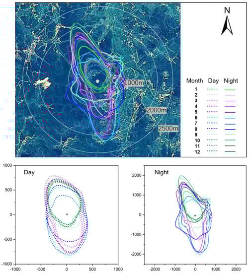
Figure 1.
The 80% monthly footprint climatologies in daytime and nighttime were calculated from 2003 to 2010 over the study area.
The footprint fetch, which is the distance from the point of the flux tower to an 80% contour of the monthly footprint climatology, mainly ranged from 600 to 900 m in the daytime and from 1200 to 2200 m in the nighttime (10th and 90th percentiles, Figure 2a). The source area covered about 0.34 to 0.86 km2 in the daytime and about 0.81 to 2.99 km2 at nighttime (10th and 90th percentiles, Figure 2b). Due to the monsoon climate, the study site had an asymmetric footprint climatology with footprint symmetry indices ranging from 0.22 to 0.51 in the daytime and from 0.12 to 0.34 in the nighttime (10th and 90th percentiles, Figure 2c).
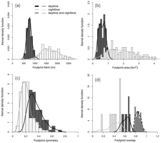
Figure 2.
Kernel density distribution of footprint fetch from the 80% footprint climatology contour (a), the source area within the 80% footprint climatology contour (b), the footprint symmetry index (c) and the footprint overlap index for seasonal and daytime–nighttime overlaps (d).
For the overlap index between daytime and nighttime (Oday_night), all the months during the study period were greater than 0.75, and 80% of them were greater than 0.8, which indicates the footprint climatologies of daytime and nighttime overlapped largely. The seasonal overlap index of daytime (Oseason_day) was higher than that of nighttime (Oseason_night). During the study period, all eight years had Oseason_day greater than 0.5, but only three years had Oseason_night greater than 0.5 (Figure 2d), which indicates intense monthly variations in footprint climatology throughout the whole year.
3.2. Spatial Heterogeneity over the Study Site
The coniferous plantation is the target vegetation for EC flux measurements and also the dominant vegetation type (70.08%) in a 6 × 6 km grid around the flux tower (Figure 3). In addition to forest, the study area is also composed of cropland (double-cropped rice, 27.83%), grassland (1.84%), waterbody (0.11%) and building (0.14%). The cropland was mainly distributed in the valley and located in the east. The double-cropped rice had a higher seasonal variation in the EVI than the coniferous plantations over the study area. During the growing season (May to October), double-cropped rice had higher EVIs than coniferous plantations, although the EVI drops during the harvest time. During the non-growing season, however, the EVI of double-cropped rice was lower than the coniferous plantation (Figure 4).
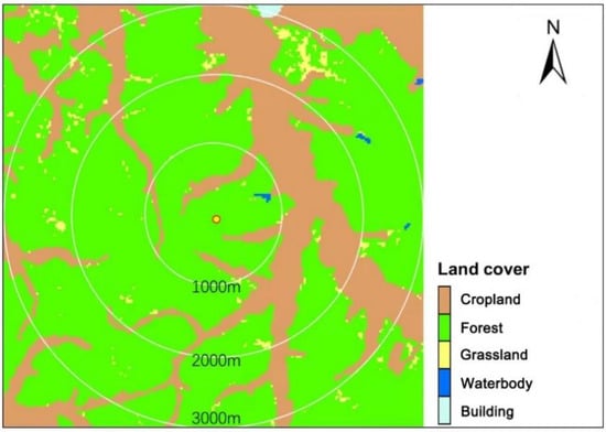
Figure 3.
The land cover map over the flux site. In a 6 × 6 km grid around the flux tower, the study area was mainly composed of forest (coniferous plantation, 70.08%), cropland (double-cropped rice, 27.83%), grassland (1.84%), waterbody (0.11%) and building (0.14%).
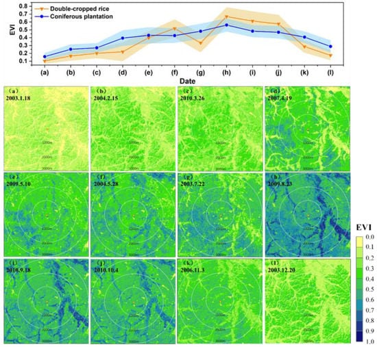
Figure 4.
Seasonal variation in EVIs from the double-cropped rice and the coniferous plantation in different months (the upper figure) and their spatial variation in EVIs over the flux site (the lower figures (a–l)). The symbols (a–l) in the upper figure are consistent with them in the lower figures. For example, the symbol (a) means 18 January 2003.
To detect the changes in spatial heterogeneity along with the increasing scales, the FTVT in a circular window with an increasing size from 250 to 3000 m was calculated based on the land cover map (Figure 5). As more double-cropped rice was included with the increasing window size, the FTVT began with 0.93 and decreased to the bottom with 0.67 at 1600 m. Then, followed by more coniferous plantations being included, the FTVT began to increase slightly and reached 0.73 at 3000 m.
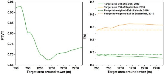
Figure 5.
Changes of FTVT and EVI in a circular window with an increasing size from 300 to 3000 m.
The average EVI in the circular window was also calculated, and the trend of the EVI showed opposite trends in the growing and non-growing seasons (Figure 5). In the growing season (September 2010), due to the increasing fraction of the double-cropped rice, the EVI generally increased and was higher than the footprint-weighted EVI over the source area. While in the non-growing season (March 2010), the EVI decreased and was lower than the footprint-weighted EVI.
3.3. Spatial Representativeness with Target Vegetation Type
For the whole study period from 2003 to 2010, the distribution of the FTVT varied greatly along the wind direction. The FTVT was 0.89 when the wind direction was southwest but reduced to 0.65 when the wind direction changed to northeast due to the larger fraction of double-cropped rice in the east part of the flux site (Figure 6).
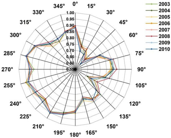
Figure 6.
Distributions of yearly FTVT, along with wind directions from 2003 to 2010.
Influenced by the monsoon climate, the source areas of the EC measurements were mainly concentrated in the southeast part in summer, and there was more coniferous plantation. In the non-growing season, however, the main wind direction was north and northwest. The source areas were mixed with more double-cropped rice. Therefore, the FTVT exhibited a single-peak seasonal variation from 2003 to 2010, which was higher in the growing season (May to September) than that in the non-growing season (Figure 7). The mean value of the FTVT ranged from 0.8254 to 0.8391, with a seasonal variation ranging from 0.0783 to 0.1416. Meanwhile, the FTVT from July 2006 was lower than the other years (Table 1). Compared with the other years, the source area of that month in 2006 was biased to the northeast, where more double-cropped rice was mixed in.
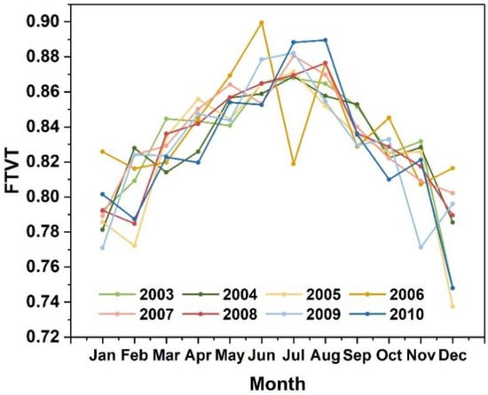
Figure 7.
Seasonal variation of FTVT from 2003 to 2010.

Table 1.
Statistics of monthly FTVT from 2003 to 2010.
3.4. Spatial Representativeness with Vegetation Index
The multi-year averaged EVIbias showed a significant monthly variation and ranged from −14.21% to 19.04% in a circular window with an increasing size from 250 to 3000 m (Figure 8a). The EVIbias in April and July ranged from 2.52% to 9.79% and fluctuated around 0. In January, March and November, the EVIbias generally increased with fluctuations and ranged from −1.42% to 11.06%. While February and December had the highest EVIbias, which ranged from 3.22% to 19.04%, where the EVIbias still increased with fluctuations. In contrast, May, August, September and October had a lower EVIbias. The EVIbias showed a decreasing trend and ranged from 10.97% to 11.06%. In June, the EVIbias was the lowest and ranged from −14.21% to 2.07%, which decreased at the beginning and remained constant after 1600 m.
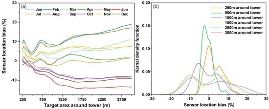
Figure 8.
Sensor location bias of EVI (EVIbias) for different months ranging from 30 to 3000 m (a) and kernel density distribution of the multi-year averaged EVIbias for circles in 250 m, 500 m, 1000 m, 1500 m, 2000 m and 3000 m (b).
The percentage of the value of the multi-year averaged EVIbias within the ±5% and ±10% thresholds were 68% and 95%, respectively, at a 250 m target area. Then, the percentages increased to 97% and 100%, respectively, at a 500 m target area. After that, the percentages decreased as the target areas increased, reaching 17% and 67%, respectively, at a 3000 m target area (Figure 8b).
4. Discussion
As the study site is located in a subtropical monsoon area [35,44], the source areas of the EC measurements had a contrary distribution direction in summer and winter. Similar results of this site were also found in other studies with different footprint models [31,63,64,65]. Chen et al. developed an upscaling framework of the EC flux for the Qianyanzhou site with the assistance of footprint modeling and remote sensing images [31]. However, the footprint awareness of the long-term EC measurement is still not receiving enough attention. There is still a need to analyze the effects of spatial heterogeneity on the spatial representativeness of EC measurements. In this study, we investigated the spatial representativeness of eight-year EC measurements under the influence of monsoon climate and analyzed the temporal variation of the spatial representativeness in the context of target vegetation type and sensor location bias, respectively.
4.1. Implications for Ecosystem Respiration and Upscaling of Flux Measurements
Although the source area of a nighttime footprint is larger than that of daytime due to the influence of atmospheric stability, the overlap areas between daytime and nighttime still account for a large proportion (Figure 2d). These largely overlapped source areas will be beneficial to the partitioning of the net exchange change (NEE) into ecosystem respiration and gross primary production (GPP). Therefore, the Oday_night can potentially be a quality flag to the GPP derived from EC flux data. The Oseason_day and Oseason_night represent the degree to which monthly footprint climatologies of daytime or nighttime overlapped in a year. Their low values indicated large differences in the spatial distribution of the source areas (Figure 2d), which is the root cause of the strong seasonal variation of spatial representation with the FTVT or EVIbias in the part of the results (Figure 7 and Figure 8). Hence, these indices can be used to detect the seasonal consistency of the source area distribution.
The upscaling of the EC measurements provides an independent approach to quantifying the carbon and water exchange between terrestrial ecosystems and the atmosphere [66]. A commonly used approach for upscaling is to integrate the flux measurements with a remote sensing model. However, biases would be introduced by the assumption that the EC measurement represents a fixed area near the flux tower site [32]. To better connect the EC measurements with remote sensing grids, the temporal variation and spatial heterogeneity of the source area should be noticed at the same time. Recent studies integrated the footprint weighting with the vegetation or land surface properties to upscale the site-level flux data to a region. Fu et al. used a footprint-weighting method to optimize a regression-based NEE-diagnosed model [67]. By integrating with high spatial-temporal resolution remote sensing data, 16 flux sites in North America were upscaled to a continental scale in their study. Serafimovich et al. related the footprint-weighted surface properties to the sensible heat flux and latent heat flux observations taken from airborne properties [68]. With a boosted regression tree technique, these fluxes were then upscaled to high-resolution flux maps over the North Slope of Alaska. Reuss-Schmidt et al. evaluated the effect of varying flux footprints on CH4 flux observation [69]. In their study, the normalized difference water index was determined to infer the representativeness of CH4 flux. Junttila et al. adopted a regression model to upscale the EC-measured GPP and ER of peatland with remote sensing data [70]. In their work, the daily vegetation and water indices derived from high-resolution Sentinel-2 data were weighted by the footprint model to match them with EC observations. Hence, we can conclude that high spatial and temporal resolution vegetation maps and indices are highly needed to upscale surface flux.
4.2. Significance of Understanding Spatial Heterogeneity and Footprint Modeling
The spatial heterogeneity of underlying surfaces contributes largely to the differences and uncertainties of flux measurements and also greatly affects the spatial representativeness [71,72]. The spatial heterogeneity can be inferred by the detailed information on vegetation or land cover properties derived from high spatial resolution satellite images within the flux source area [27]. Therefore, the spatial heterogeneity of flux can be better recognized by integrating high spatial resolution remote sensing images and footprint analyses [73]. The spatial representation of flux data can be improved by utilizing footprint information and high spatial resolution remote sensing images. Barcza et al. extracted crop-specific flux by applying a detailed footprint analysis [74]. Sánchez et al. improved the energy closure by 5% after filtering out the flux data from bare soil in a boreal forest flux site in Finland [23]. Tuovinen et al. decomposed methane flux of Siberian tundra into land-cover-specific data by footprint weighting and wind direction [27].
Mismatching between the local scale EC observations with a temporally varying flux footprint and regional scale gridded estimation is a major issue in model-data comparisons [75]. To solve this issue, a feasible way is to acquire daily “ground truth” data based on footprint models at a remote sensing pixel scale [76]. Meanwhile, footprint modeling has been widely used in recent years to solve another mismatch issue between measurements from plot-scale chambers and footprint-scale ECs. Budishchev et al. used a footprint-weighted average method to evaluate a plot-scale methane emission model with EC measurements [77]. With the help of this footprint-weighted method, the daily dynamics of EC flux were properly captured by the plot-scale model. Kade et al. improved the consistency of the measurements from the chamber and EC by using detailed vegetation maps and footprint analyses [78]. The footprint modeling is expected to be a bridge connecting the flux observations from the plot, EC footprint and regional grid scale.
On the other hand, the change in remote sensing gird can also lead to the mismatch issue. Many studies show that solar-induced chlorophyll fluorescence (SIF) is closely related to the plant photosynthetic rate and plant physiological state [79,80,81,82]. Here, SIF pixels from the Global Ozone Monitoring Experiment-2 (GOME-2) [83,84], in October 2010, were chosen to be compared with the footprint-weighted EVI and FTVT on the same day to demonstrate to what degree the change in remote sensing pixel position can lead to in mismatch issue (Figure 9 and Figure 10). There is little difference in the EVIs between the two, but there is a great difference in the FTVT (Table 2 and Table 3). This indicates that the flux information of the two with similar fluxes may not come from the same vegetation type, and the heterogeneity between vegetation types should be fully considered when addressing the mismatch issue.
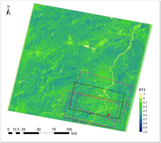
Figure 9.
The location of the study site (red point) and the rectangular area is the solar-induced chlorophyll fluorescence (SIF) pixel (40 km × 80 km) of the Global Ozone Monitoring Experiment-2 (GOME-2) in the same period, and the background is an EVI image derived from Landsat TM, 4 th October 2010. It can be seen that the SIF pixel position shift of GOME-2 is large, and the value of EVI within each pixel is relatively different.
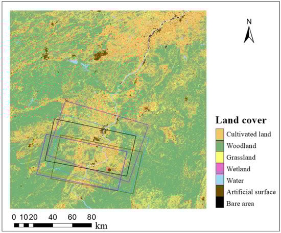
Figure 10.
The location of the study site (red point) and the rectangular area is the solar-induced chlorophyll fluorescence (SIF) pixel (40 km × 80 km) of the Global Ozone Monitoring Experiment-2 (GOME-2) in the same period, and the background is a land cover image derived from GlobeLand30. It can be seen that the vegetation type in SIF pixels is mainly cultivated land, and the composition proportion of each vegetation type still changed.
Table 2.
Comparison of EVI within the flux source area and the pixels of GOME-2 SIF data.
Table 3.
Comparison of FTVT within the flux source area and the pixels of GOME-2 SIF data.
4.3. Implications of Remote Sensing Products
Detailed and accurate land cover maps are essential for capturing vegetation information over heterogeneous underlying surfaces [85]. The high-resolution remote sensing images obtained from unmanned aerial vehicles (UAV), airborne or satellite, are therefore particularly important in footprint analysis. However, remote sensing images with high spatial resolution usually have a lower temporal resolution. In fact, there is a trade-off between the grid resolution and revisit frequency for remote sensing images. The spatial and temporal resolution should be considered comprehensively. Hence, Landsat series images are still the most commonly used dataset to track the long-term changes in spatial representativeness and to compare the spatial representativeness across flux sites [25,26,31,32].
5. Conclusions
In this study, the variations in spatial representativeness of the EC measurements were evaluated by using eight-year continuous flux data and remote sensing images in a subtropical coniferous plantation site of a monsoon area. We found that the spatial representativeness had been affected by the monsoon climate and the spatial heterogeneity around the flux site. Although the coniferous plantation was the dominant vegetation type over the flux site, the mixing of double-cropped rice changed the spatial representation significantly during a year. Our study demonstrates the effects of spatial heterogeneity on the spatial representation of EC measurements and highlights the importance of footprint awareness in the utilization of EC measurements for calibrating and validating EC data in a model.
Author Contributions
W.X. was the principal investigator for this study. He undertook data processing, carried out the main data analyses, and wrote the manuscript. X.R. contributed to the interpretation and presentation of the statistical results and revised the text. W.Y. and X.Q. assisted and contributed to the interpretation and presentation of the statistical results. S.J. assisted and contributed to the data analysis. H.W. was the main supervisor for the project. He supervised the work and helped in developing the methodology for the study, interpreting the results, and revising earlier drafts until the final approval. J.A. was the co-supervisor for the project. He assisted with developing the methodology for the study, supervised the development of the model, and revised the text. All authors have read and agreed to the published version of the manuscript.
Funding
This research was funded by the National Key Research and Development Program of China (Grant No. 2020YFA0608103) and the National Science Foundation of China (Grant No. 31770765, 32160366).
Data Availability Statement
Not applicable.
Acknowledgments
We thank the Qianyanzhou Ecological Research Station, which is a CERN and ChinaFLUX site, for sharing their data.
Conflicts of Interest
The authors declare no conflict of interest.
References
- Lowry, A.L.; McGowan, H.A.; Gray, M.A. Multi-year carbon and water exchanges over contrasting ecosystems on a sub-tropical sand island. Agric. For. Meteorol. 2021, 304–305, 108404. [Google Scholar] [CrossRef]
- Running, S.; Baldocchi, D.; Turner, D.; Gower, S.; Bakwin, P.; Hibbard, K. A Global Terrestrial Monitoring Network Integrating Tower Fluxes, Flask Sampling, Ecosystem Modeling and EOS Satellite Data. Remote Sens. Environ. 1999, 70, 108–127. [Google Scholar] [CrossRef]
- Mu, Q.; Zhao, M.; Running, S.W. Improvements to a MODIS global terrestrial evapotranspiration algorithm. Remote Sens. Environ. 2011, 115, 1781–1800. [Google Scholar] [CrossRef]
- Chen, L.; Dirmeyer, P.A.; Guo, Z.; Schultz, N.M. Pairing FLUXNET sites to validate model representations of land-use/land-cover change. Hydrol. Earth Syst. Sci. 2018, 22, 111–125. [Google Scholar] [CrossRef]
- Ricciuto, D.; Sargsyan, K.; Thornton, P. The Impact of Parametric Uncertainties on Biogeochemistry in the E3SM Land Model. J. Adv. Model. Earth Syst. 2018, 10, 297–319. [Google Scholar] [CrossRef]
- Aubinet, M.; Grelle, A.; Ibrom, A.; Rannik, U.; Moncrieff, J.; Foken, T.; Kowalski, A.S.; Martin, P.H.; Berbigier, P.; Bernhofer, C.; et al. Estimates of the annual net carbon and water exchange of forests: The EUROFLUX methodology. Adv. Ecol. Res. 1999, 30, 113–175. [Google Scholar] [CrossRef]
- Baldocchi, D.D.; Falge, E.; Gu, L.H.; Olson, R.; Hollinger, D.; Running, S.; Anthoni, P.; Bernhofer, C.; Davis, K.; Evans, R.; et al. FLUXNET: A new tool to study the temporal and spatial variability of ecosystem-scale carbon dioxide, water vapor, and energy flux densities. Bull. Am. Meteorol. Soc. 2001, 82, 2415–2434. [Google Scholar] [CrossRef]
- Law, B.; Falge, E.; Gu, L.; Baldocchi, D.; Bakwin, P.; Berbigier, P.; Davis, K.; Dolman, A.; Falk, M.; Fuentes, J.; et al. Environmental controls over carbon dioxide and water vapor exchange of terrestrial vegetation. Agric. For. Meteorol. 2002, 113, 97–120. [Google Scholar] [CrossRef]
- Baldocchi, D.D. How eddy covariance flux measurements have contributed to our understanding of Global Change Biology. Glob. Chang. Biol. 2020, 26, 242–260. [Google Scholar] [CrossRef]
- Yao, Y.; Liang, S.; Li, X.; Chen, J.; Liu, S.; Jia, K.; Zhang, X.; Xiao, Z.; Fisher, J.B.; Mu, Q.; et al. Improving global terrestrial evapotranspiration estimation using support vector machine by integrating three process-based algorithms. Agric. For. Meteorol. 2017, 242, 55–74. [Google Scholar] [CrossRef]
- Badgley, G.; Anderegg, L.D.L.; Berry, J.A.; Field, C.B. Terrestrial gross primary production: Using NIRV to scale from site to globe. Glob. Chang. Biol. 2019, 25, 3731–3740. [Google Scholar] [CrossRef]
- Zhang, Y.; Kong, D.; Gan, R.; Chiew, F.H.S.; McVicar, T.R.; Zhang, Q.; Yang, Y. Coupled estimation of 500 m and 8-day resolution global evapotranspiration and gross primary production in 2002–2017. Remote Sens. Environ. 2019, 222, 165–182. [Google Scholar] [CrossRef]
- Cai, W.J.; Prentice, L.C. Recent trends in gross primary production and their drivers: Analysis and modelling at flux-site and global scales Environ. Res. Lett. 2020, 15, 124050. [Google Scholar] [CrossRef]
- Elnashar, A.; Wang, L.; Wu, B.; Zhu, W.; Zeng, H. Synthesis of global actual evapotranspiration from 1982 to 2019. Earth Syst. Sci. Data 2021, 13, 447–480. [Google Scholar] [CrossRef]
- Pan, X.X.; Lei, H.M.; Cong, Z.T.; Yang, H.B.; Duan, L.M.; Yang, D.W. Long term variation of evapotranspiration and water balance based on upscaling eddy covariance observations over the temperate semi-arid grassland of China. Agric. For. Meterol. 2021, 308–309, 108566. [Google Scholar]
- Tagesson, T.; Tian, F.; Schurgers, G.; Horion, S.; Scholes, R.; Ahlström, A.; Ardö, J.; Moreno, A.; Madani, N.; Olin, S.; et al. A physiology-based Earth observation model indicates stagnation in the global gross primary production during recent decades. Glob. Chang. Biol. 2021, 27, 836–854. [Google Scholar] [CrossRef] [PubMed]
- Wang, Z.; Liu, S.; Wang, Y.; Valbuena, R.; Wu, Y.; Kutia, M.; Zheng, Y.; Lu, W.; Zhu, Y.; Zhao, M.; et al. Tighten the Bolts and Nuts on GPP Estimations from Sites to the Globe: An Assessment of Remote Sensing Based LUE Models and Supporting Data Fields. Remote Sens. 2021, 13, 168. [Google Scholar] [CrossRef]
- Schmid, H.P.; Lloyd, C.R. Spatial representativeness and the location bias of flux footprints over inhomogeneous areas. Agric. For. Meteorol. 1999, 93, 195–209. [Google Scholar] [CrossRef]
- Gelybó, G.; Barcza, Z.; Kern, A.; Kljun, N. Effect of spatial heterogeneity on the validation of remote sensing based GPP estimations. Agric. For. Meteorol. 2013, 174–175, 43–53. [Google Scholar] [CrossRef]
- Schuepp, P.H.; Leclerc, M.Y.; MacPherson, J.I.; Desjardins, R.L. Footprint prediction of scalar fluxes from analytical solutions of the diffusion equation. Bound.-Layer Meteorol. 1990, 50, 355–373. [Google Scholar] [CrossRef]
- Schmid, H. Experimental design for flux measurements: Matching scales of observations and fluxes. Agric. For. Meteorol. 1997, 87, 179–200. [Google Scholar] [CrossRef]
- Yi, C. Momentum Transfer within Canopies. J. Appl. Meteorol. Clim. 2008, 47, 262–275. [Google Scholar] [CrossRef]
- Sánchez, J.M.; Caselles, V.; Rubio, E.M. Analysis of the energy balance closure over a FLUXNET boreal forest in Finland. Hydrol. Earth Syst. Sci. 2010, 14, 1487–1497. [Google Scholar] [CrossRef]
- Chen, B.; Coops, N.C.; Fu, D.; Margolis, H.A.; Amiro, B.D.; Black, T.A.; Arain, M.A.; Barr, A.G.; Bourque, C.P.-A.; Flanagan, L.; et al. Characterizing spatial representativeness of flux tower eddy-covariance measurements across the Canadian Carbon Program Network using remote sensing and footprint analysis. Remote Sens. Environ. 2012, 124, 742–755. [Google Scholar] [CrossRef]
- Wang, H.; Jia, G.; Zhang, A.; Miao, C. Assessment of Spatial Representativeness of Eddy Covariance Flux Data from Flux Tower to Regional Grid. Remote Sens. 2016, 8, 742. [Google Scholar] [CrossRef]
- Kim, J.; Hwang, T.; Schaaf, C.L.; Kljun, N.; Munger, J.W. Seasonal variation of source contributions to eddy-covariance CO2 measurements in a mixed hardwood-conifer forest. Agric. For. Meteorol. 2018, 253–254, 71–83. [Google Scholar] [CrossRef]
- Tuovinen, J.-P.; Aurela, M.; Hatakka, J.; Räsänen, A.; Virtanen, T.; Mikola, J.; Ivakhov, V.; Kondratyev, V.; Laurila, T. Interpreting eddy covariance data from heterogeneous Siberian tundra: Land-cover-specific methane fluxes and spatial representativeness. Biogeosciences 2019, 16, 255–274. [Google Scholar] [CrossRef]
- Su, Z. The Surface Energy Balance System (SEBS) for estimation of turbulent heat fluxes. Hydrol. Earth Syst. Sci. 2002, 6, 85–100. [Google Scholar] [CrossRef]
- Wylie, B.K.; Johnson, D.A.; Laca, E.; Saliendra, N.Z.; Gilmanovd, T.G.; Reed, B.C.; Tieszen, L.L.; Worstell, B.B. Calibration of remotely sensed, coarse resolution NDVI to CO2 fluxes in a sagebrush–steppe ecosystem. Remote Sens. Environ. 2003, 85, 243–255. [Google Scholar] [CrossRef]
- Sims, D.A.; Rahman, A.F.; Cordova, V.D.; El-Masri, B.Z.; Baldocchi, D.D.; Bolstad, P.V.; Flanagan, L.B.; Goldstein, A.H.; Hollinger, D.Y.; Misson, L.; et al. A new model of gross primary productivity for North American ecosystems based solely on the enhanced vegetation index and land surface temperature from MODIS. Remote Sens. Environ. 2008, 112, 1633–1646. [Google Scholar] [CrossRef]
- Chen, B.; Ge, Q.; Fu, D.; Yu, G.; Sun, X.; Wang, S.; Wang, H. A data-model fusion approach for upscaling gross ecosystem productivity to the landscape scale based on remote sensing and flux footprint modelling. Biogeosciences 2010, 7, 2943–2958. [Google Scholar] [CrossRef]
- Chu, H.; Luo, X.; Ouyang, Z.; Chan, W.S.; Dengel, S.; Biraud, S.C.; Torn, M.S.; Metzger, S.; Kumar, J.; Arain, M.A.; et al. Representativeness of Eddy-Covariance flux footprints for areas surrounding AmeriFlux sites. Agric. For. Meteorol. 2021, 301–302, 108350. [Google Scholar] [CrossRef]
- Chen, B.; Coops, N.C.; Fu, D.; Margolis, H.A.; Amiro, B.D.; Barr, A.G.; Black, T.A.; Arain, M.A.; Bourque, C.P.-A.; Flanagan, L.B.; et al. Assessing eddy-covariance flux tower location bias across the Fluxnet-Canada Research Network based on remote sensing and footprint modelling. Agric. For. Meteorol. 2011, 151, 87–100. [Google Scholar] [CrossRef]
- Chen, C.; Park, T.; Wang, X.; Piao, S.; Xu, B.; Chaturvedi, R.K.; Fuchs, R.; Brovkin, V.; Ciais, P.; Fensholt, R.; et al. China and India lead in greening of the world through land-use management. Nat. Sustain. 2019, 2, 122–129. [Google Scholar] [CrossRef]
- Wen, X.-F.; Wang, H.-M.; Wang, J.-L.; Yu, G.-R.; Sun, X.-M. Ecosystem carbon exchanges of a subtropical evergreen coniferous plantation subjected to seasonal drought, 2003–2007. Biogeosciences 2010, 7, 357–369. [Google Scholar] [CrossRef]
- Tan, Z.-H.; Zhang, Y.-P.; Song, Q.-H.; Liu, W.-J.; Deng, X.-B.; Tang, J.-W.; Deng, Y.; Zhou, W.-J.; Yang, L.-Y.; Yu, G.-R.; et al. Rubber plantations act as water pumps in tropical China. Geophys. Res. Lett. 2011, 38, L24406. [Google Scholar] [CrossRef]
- Tong, X.; Meng, P.; Zhang, J.; Li, J.; Zheng, N.; Huang, H. Ecosystem carbon exchange over a warm-temperate mixed plantation in the lithoid hilly area of the North China. Atmos. Environ. 2012, 49, 257–267. [Google Scholar] [CrossRef]
- Tong, X.; Zhang, J.; Meng, P.; Li, J.; Zheng, N. Ecosystem water use efficiency in a warm-temperate mixed plantation in the North China. J. Hydrol. 2014, 512, 221–228. [Google Scholar] [CrossRef]
- Zhou, J.; Zhang, Z.; Sun, G.; Fang, X.; Zha, T.; McNulty, S.; Chen, J.; Jin, Y.; Noormets, A. Response of ecosystem carbon fluxes to drought events in a poplar plantation in Northern China. For. Ecol. Manag. 2013, 300, 33–42. [Google Scholar] [CrossRef]
- Sun, S.; Meng, P.; Zhang, J.; Wan, X.; Zheng, N.; He, C. Partitioning oak woodland evapotranspiration in the rocky mountainous area of North China was disturbed by foreign vapor, as estimated based on non-steady-state 18O isotopic composition. Agric. For. Meteorol. 2014, 184, 36–47. [Google Scholar] [CrossRef]
- Gao, S.; Chen, J.; Tang, Y.; Xie, J.; Zhang, R.; Tang, J.; Zhang, X. Ecosystem carbon (CO2 and CH4) fluxes of a Populus dettoides plantation in subtropical China during and post clear-cutting. For. Ecol. Manag. 2015, 357, 206–219. [Google Scholar] [CrossRef]
- Xi, B.; Di, N.; Wang, Y.; Duan, J.; Jia, L. Modeling stand water use response to soil water availability and groundwater level for a mature Populus tomentosa plantation located on the North China Plain. For. Ecol. Manag. 2017, 391, 63–74. [Google Scholar] [CrossRef]
- Ma, J.; Jia, X.; Zha, T.; Bourque, C.P.-A.; Tian, Y.; Bai, Y.; Liu, P.; Yang, R.; Li, C.; Li, C.; et al. Ecosystem water use efficiency in a young plantation in Northern China and its relationship to drought. Agric. For. Meteorol. 2019, 275, 1–10. [Google Scholar] [CrossRef]
- Wen, X.-F.; Yu, G.-R.; Sun, X.-M.; Li, Q.-K.; Liu, Y.-F.; Zhang, L.-M.; Ren, C.-Y.; Fu, Y.-L.; Li, Z.-Q. Soil moisture effect on the temperature dependence of ecosystem respiration in a subtropical Pinus plantation of southeastern China. Agric. For. Meteorol. 2006, 137, 166–175. [Google Scholar] [CrossRef]
- Xu, K.; Metzger, S.; Desai, A.R. Upscaling tower-observed turbulent exchange at fine spatio-temporal resolution using environmental response functions. Agric. For. Meteorol. 2017, 232, 10–22. [Google Scholar] [CrossRef]
- Chen, C.H.; Wei, J.; Wen, X.F.; Sun, X.M.; Guo, Q.J. Photosynthetic carbon isotope discrimination and effects on daytime nee partitioning in a subtropical mixed conifer plantation. Agric. For. Meteorol. 2019, 272–273, 143–155. [Google Scholar] [CrossRef]
- Zhang, W.; Wang, H.; Wen, X.; Yang, F.; Ma, Z.; Sun, X.; Yu, G. Freezing-induced loss of carbon uptake in a subtropical coniferous plantation in southern China. Ann. For. Sci. 2011, 68, 1151–1161. [Google Scholar] [CrossRef][Green Version]
- Ma, Z.; Hartmann, H.; Wang, H.; Li, Q.; Wang, Y.; Li, S. Carbon dynamics and stability between native Masson pine and exotic slash pine plantations in subtropical China. Forstwiss. Cent. 2014, 133, 307–321. [Google Scholar] [CrossRef]
- Dai, X.Q.; Wang, H.M.; Xu, M.J.; Yang, F.T.; Wen, X.F.; Chen, Z.; Zhang, L.M.; Sun, X.M.; Yu, G.R. An Observation Dataset of Carbon and Water Fluxes of Artificial Coniferous Forests in Qianyanzhou (2003–2010); Science Data Bank: Beijing, China, 2020. [Google Scholar]
- Zhang, L.; Luo, Y.; Chen, Z.; Su, W.; He, H.; Zhu, Z.; Sun, X.; Wang, Y.; Zhou, G.; Zhao, X.; et al. Carbon and Water Fluxes Observed by the Chinese Flux Observation and Research Network (2003–2005); Science Data Bank: Beijing, China, 2018. [Google Scholar] [CrossRef]
- Aubinet, M.; Vesala, T.; Papale, D. (Eds.) Eddy Covariance: A Practical Guide to Measurement and Data Analysis Series; Springer: Dordrecht, The Netherlands, 2012. [Google Scholar]
- Schotanus, P.; Nieuwstadt, F.T.M.; De Bruin, H.R. Temperature measurement with a sonic anemometer and its application to heat and moisture fluxes. Boundary-Layer Meteorol. 1983, 26, 81–93. [Google Scholar] [CrossRef]
- Wilczak, J.M.; Oncley, S.P.; Stage, S.A. Sonic Anemometer Tilt Correction Algorithms. Boundary-Layer Meteorol. 2001, 99, 127–150. [Google Scholar] [CrossRef]
- Webb, E.K.; Pearman, G.I.; Leuning, R. Correction of the flux measurements for density effects due to heat and water vapor transfer. Q. J. R. Meteorol. Soc. 1980, 106, 85–100. [Google Scholar] [CrossRef]
- Moore, C.J. Frequency response corrections for eddy correlation systems. Boundary-Layer Meteorol. 1986, 37, 17–35. [Google Scholar] [CrossRef]
- Hollinger, D.Y.; Kelliher, F.M.; Byers, J.N.; Hunt, J.E.; McSeveny, T.M.; Weir, P.L. Carbon dioxideexchange between an undisturbed old-growth temperate forest and the atmosphere. Ecology 1994, 75, 134–150. [Google Scholar] [CrossRef]
- Foken, T.; Leuning, R.; Oncley, S.R.; Mauder, M.; Aubinet, M. Corrections and data quality. In Eddy Covariance: A Practical Guide to Measurement and Data Analysis; Aubinet, M., Vesala, T., Papale, D., Eds.; Springer: Dordrecht, The Netherlands, 2012; pp. 85–131. [Google Scholar]
- Reichstein, M.; Falge, E.; Baldocchi, D.; Papale, D.; Aubinet, M.; Berbigier, P.; Bernhofer, C.; Buchmann, N.; Gilmanov, T.; Granier, A.; et al. On the separation of net ecosystem exchange into assimilation and ecosystem respiration: Review and improved algorithm. Glob. Chang. Biol. 2005, 11, 1424–1439. [Google Scholar] [CrossRef]
- Papale, D.; Valentini, R. A new assessment of European forests carbon exchanges by eddy fluxes and artificial neural network spatialization. Glob. Chang. Biol. 2003, 9, 525–535. [Google Scholar] [CrossRef]
- Jun, C.; Ban, Y.; Li, S. Open access to Earth land-cover map. Nature 2014, 514, 434. [Google Scholar] [CrossRef]
- Huete, A.; Didan, K.; Miura, T.; Rodriguez, E.P.; Gao, X.; Ferreira, L.G. Overview of the radiometric and biophysical performance of the MODIS vegetation indices. Remote Sens. Environ. 2002, 83, 195–213. [Google Scholar] [CrossRef]
- Kljun, N.; Calanca, P.; Rotach, M.W.; Schmid, H.P. A simple two-dimensional parameterisation for Flux Footprint Prediction (FFP). Geosci. Model Dev. 2015, 8, 3695–3713. [Google Scholar] [CrossRef]
- Mi, N.; Yu, G.; Wang, P.; Wen, X.; Sun, X. A preliminary study for spatial representiveness of flux observation at ChinaFLUX sites. Sci. China Ser. D Earth Sci. 2006, 49 (Supp. II), 24–35. [Google Scholar] [CrossRef]
- Zhang, W.-J.; Wang, H.-M.; Yang, F.-T.; Yi, Y.-H.; Wen, X.-F.; Sun, X.-M.; Yu, G.-R.; Wang, Y.-D.; Ning, J.-C. Underestimated effects of low temperature during early growing season on carbon sequestration of a subtropical coniferous plantation. Biogeosciences 2011, 8, 1667–1678. [Google Scholar] [CrossRef]
- Zhang, H.; Wen, X. Flux footprint climatology estimated by three analytical models over a subtropical coniferous plantation in Southeast China. J. Meteorol. Res. 2015, 29, 654–666. [Google Scholar] [CrossRef]
- Xiao, J.; Chen, J.; Davis, K.J.; Reichstein, M. Advances in upscaling of eddy covariance measurements of carbon and water fluxes. J. Geophys. Res. 2012, 117. [Google Scholar] [CrossRef]
- Fu, D.J.; Chen, B.Z.; Zhang, H.F.; Wang, J.; Black, T.A.; Amiro, B.D.; Bohrer, G.; Bolstad, P.; Coulter, R.; Rahman, A.F.; et al. Estimating landscape net ecosystem exchange at high spatial-temporal resolution based on landsat data, an improved upscaling model framework, and eddy covariance flux measurements. Remote Sens. Environ. 2014, 141, 90–104. [Google Scholar] [CrossRef]
- Serafimovich, A.; Metzger, S.; Hartmann, J.; Kohnert, K.; Zona, D.; Sachs, T. Upscaling surface energy fluxes over the North Slope of Alaska using airborne eddy-covariance measurements and environmental response functions. Atmos. Chem. Phys. 2018, 18, 10007–10023. [Google Scholar] [CrossRef]
- Reuss-Schmidt, K.; Levy, P.E.; Oechel, W.; Tweedie, C.E.; Wilson, C.J.; Zona, D. Understanding spatial variability of methane fluxes in Arctic wetlands through footprint modelling. Environ. Res. Lett. 2019, 14, 125010. [Google Scholar] [CrossRef]
- Junttila, S.; Kelly, J.; Kljun, N.; Aurela, M.; Klemedtsson, L.; Lohila, A.; Nilsson, M.; Rinne, J.; Tuittila, E.-S.; Vestin, P.; et al. Upscaling Northern Peatland CO2 Fluxes Using Satellite Remote Sensing Data. Remote Sens. 2021, 13, 818. [Google Scholar] [CrossRef]
- Sun, G.; Hu, Z.; Sun, F.; Wang, J.; Xie, Z.; Lin, Y.; Huang, F. An analysis on the influence of spatial scales on sensible heat fluxes in the north Tibetan Plateau based on Eddy covariance and large aperture scintillometer data. Arch. Meteorol. Geophys. Bioclimatol. Ser. B 2016, 129, 965–976. [Google Scholar] [CrossRef]
- El-Madany, T.S.; Reichstein, M.; Perez-Priego, O.; Carrara, A.; Moreno, G.; Martín, M.P.; Pacheco-Labrador, J.; Wohlfahrt, G.; Nieto, H.; Weber, U.; et al. Drivers of spatio-temporal variability of carbon dioxide and energy fluxes in a Mediterranean savanna ecosystem. Agric. For. Meteorol. 2018, 262, 258–278. [Google Scholar] [CrossRef]
- Hannun, R.A.; Wolfe, G.M.; Kawa, S.R.; Hanisco, T.F.; Newman, P.A.; Alfieri, J.G.; Barrick, J.D.; Clark, K.L.; DiGangi, J.P.; Diskin, G.S.; et al. Spatial heterogeneity in CO2, CH4, and energy fluxes: Insights from airborne eddy covariance measurements over the Mid-Atlantic region. Environ. Res. Lett. 2020, 15, 035008. [Google Scholar] [CrossRef]
- Barcza, Z.; Kern, A.; Haszpra, L.; Kljun, N. Spatial representativeness of tall tower eddy covariance measurements using remote sensing and footprint analysis. Agric. For. Meteorol. 2009, 149, 795–807. [Google Scholar] [CrossRef]
- Xu, M.; Wang, H.; Wenjiang, Z.; Zhang, T.; Di, Y.; Wang, Y.; Wang, J.; Cheng, C.; Zhang, W. The full annual carbon balance of a subtropical coniferous plantation is highly sensitive to autumn precipitation. Sci. Rep. 2017, 7, 1–12. [Google Scholar] [CrossRef]
- Li, X.; Liu, S.; Li, H.; Ma, Y.; Wang, J.; Zhang, Y.; Xu, Z.; Xu, T.; Song, L.; Yang, X.; et al. Intercomparison of Six Upscaling Evapotranspiration Methods: From Site to the Satellite Pixel. J. Geophys. Res. Atmos. 2018, 123, 6777–6803. [Google Scholar] [CrossRef]
- Budishchev, A.; Mi, Y.; van Huissteden, J.; Belelli-Marchesini, L.; Schaepman-Strub, G.; Parmentier, F.J.W.; Fratini, G.; Gallagher, A.; Maximov, T.C.; Dolman, A.J. Evaluation of a plot-scale methane emission model using eddy covariance observations and footprint modelling. Biogeosciences 2014, 11, 4651–4664. [Google Scholar] [CrossRef]
- Kade, A.; Bret-Harte, M.S.; Euskirchen, E.S.; Edgar, C.; Fulweber, R.A. Upscaling of CO2fluxes from heterogeneous tundra plant communities in Arctic Alaska. J. Geophys. Res. Earth Surf. 2012, 117, G04007. [Google Scholar] [CrossRef]
- Damm, A.; Elbers, J.; Erler, A.; Gioli, B.; Hamdi, K.; Hutjes, R.; Kosvancova, M.; Meroni, M.; Miglietta, F.; Moersch, A.; et al. Remote sensing of sun-induced fluorescence to improve modeling of diurnal courses of gross primary production (GPP). Glob. Chang. Biol. 2010, 16, 171–186. [Google Scholar] [CrossRef]
- Damm, A.; Guanter, L.; Verhoef, W.; Schläpfer, D.; Garbari, S.; Schaepman, M. Impact of varying irradiance on vegetation indices and chlorophyll fluorescence derived from spectroscopy data. Remote Sens. Environ. 2015, 156, 202–215. [Google Scholar] [CrossRef]
- Magney, T.S.; Bowling, D.R.; Logan, B.; Grossmann, K.; Stutz, J.; Blanken, P.D.; Burns, S.P.; Cheng, R.; Garcia, M.A.; Köhler, P.; et al. Mechanistic evidence for tracking the seasonality of photosynthesis with solar-induced fluorescence. Proc. Natl. Acad. Sci. USA 2019, 116, 11640–11645. [Google Scholar] [CrossRef]
- Yang, X.; Tang, J.; Mustard, J.F.; Lee, J.-E.; Rossini, M.; Joiner, J.; Munger, J.W.; Kornfeld, A.; Richardson, A.D. Solar-induced chlorophyll fluorescence that correlates with canopy photosynthesis on diurnal and seasonal scales in a temperate deciduous forest. Geophys. Res. Lett. 2015, 42, 2977–2987. [Google Scholar] [CrossRef]
- Joiner, J.; Guanter, L.; Lindstrot, R.; Voigt, M.; Vasilkov, A.P.; Middleton, E.M.; Huemmrich, K.F.; Yoshida, Y.; Frankenberg, C. Global monitoring of terrestrial chlorophyll fluorescence from moderate-spectral-resolution near-infrared satellite measurements: Methodology, simulations, and application to GOME-2. Atmos. Meas. Tech. 2013, 6, 2803–2823. [Google Scholar] [CrossRef]
- Wolanin, A.; Rozanov, V.; Dinter, T.; Noël, S.; Vountas, M.; Burrows, J.; Bracher, A. Global retrieval of marine and terrestrial chlorophyll fluorescence at its red peak using hyperspectral top of atmosphere radiance measurements: Feasibility study and first results. Remote Sens. Environ. 2015, 166, 243–261. [Google Scholar] [CrossRef]
- Xiao, J.; Davis, K.J.; Urban, N.M.; Keller, K.; Saliendra, N.Z. Upscaling carbon fluxes from towers to the regional scale: Influence of parameter variability and land cover representation on regional flux estimates. J. Geophys. Res. 2011, 116, G00J06. [Google Scholar] [CrossRef]


Publisher’s Note: MDPI stays neutral with regard to jurisdictional claims in published maps and institutional affiliations. |
© 2022 by the authors. Licensee MDPI, Basel, Switzerland. This article is an open access article distributed under the terms and conditions of the Creative Commons Attribution (CC BY) license (https://creativecommons.org/licenses/by/4.0/).