Abstract
In recent years, marine oil spills have adversely affected the marine economy and ecosystem, and the detection of marine oil slicks has attracted great attention. Combining different polarimetric features for better oil spill detection is a topic that needs to be studied in depth. Previous studies have shown that the compact polarimetric (CP) synthetic aperture radar (SAR) can be effectively applied to the detection of sea surface oil spill due to its own ability, which is conducive to the extraction of sea surface oil slick. In this paper, we apply the power–entropy (PE) decomposition theory, which decomposes the total scattered power according to the entropy contribution of each cell in the response, to CP SAR data for oil spill detection. The purpose of this study is to enhance the oil slick and the separability of the sea. As a result, an oil spill detection method based on the low-entropy radiation amplitude parameter is proposed. We compare with the other five popular polarimetric features and validate by quantitative evaluation that is superior to other types of polarization feature parameters under different band data. Moreover, the random forest classification is performed on the feature map and achieves the visualization results of oil spill detection. The experimental results show that the can combine the information of the two polarimetric characteristic parameters of entropy and total scattering power, and can clearly indicate the oil slick information under different scenarios.
1. Introduction
With the development of industrial technology, petroleum has become the most important raw material for industrial manufacturing. At the same time, oil spills caused by the massive exploitation of oil have become a serious environmental problem. Due to the increase in maritime transport trade and the development of offshore oil platforms, the risk of environmental pollution from oil discharges has increased dramatically over the past few decades. Oil spill detection has also become an important topic among researchers [1,2,3].
Oil spill detection is enabled using full polarimetric (FP) synthetic aperture radar (SAR) data, but its main limitations are the reduced swath width and constrained span of incidence [4]. The compact polarimetry (CP) architecture [5] can provide correlation performance close to that of FP SAR while avoiding the disadvantages of FP SAR [6]. The CP mode can obtain partial polarimetric information while maintaining the swath width of dual polarimetric SAR, which makes it very suitable for large-area ocean surveillance [7]. The π/4 mode was proposed by Souyris et al. [8]. Stacy and Preiss [9] slightly modified the original compact polarimetric algorithm and proposed dual circular polarization (DCP) [10]. Further, Raney [11] proposed a hybrid-polarimetric (HP) architecture. The hybrid-polarimetric architecture transmits circular polarization but receives two orthogonal, mutually coherent linear polarizations. Notably, CP SAR data has been successfully applied to oil spill detection [12].
Liu et al. [13] proposed and compared two oil spill detection methods with four scattering matrices. The first algorithm is based on a new parameter, which is composed of the co-polar correlation coefficient and the scattering matrix decomposition parameter. The second algorithm uses the total power of the four polarimetric channels image. The result shows that both algorithms can detect oil slicks. Shirvany et al. [14] studied the performance of the degree of polarization (DoP) for oil spill detection under different polarizations in hybrid/compact and linear dual-pol SAR imagery. The results show that the hybrid/compact polarization mode is more suitable for oil spill detection than the traditional dual-polarization mode. Starting from the extended Bragg scattering model (X-Bragg), Yin et al. [15] proposed three parameters for the joint detection of oil spills and ships. The parameter, which is related to the co-pol ratio, can be derived from the Huynen parameter and is used in this study. In [16], C-band polarimetric data was used to study the capabilities of CP modes in oil spill detection, and it was shown that the circular transmit CP mode is more suitable for sea surface surveillance than the linear mode. A new detection method is proposed based on the X-Bragg model, and the analysis shows that the CP and quad-pol modes can obtain reasonably similar results in the discrimination of sea surface targets. Nunziata et al. [6] first proposed the HP architecture to detect oil slicks at sea, including DoP, entropy, circular polarization ratio, complex correlation coefficient, relative phase, and the standard deviation of the relative phase. The effectiveness of the HP architecture for oil spill detection is demonstrated. Using the structure of the compact polarimetry data in circular transmit, linear receive (CL) mode, Salberg et al. [4] deduced coherence measurement, which suppresses some similar phenomena caused by low winds while providing good oil slick contrast. The experiment shows that the HP feature provides similar performance to FP SAR in the identification of oil slicks on the sea surface. Singha et al. [17] extracted ten polarimetric parameters and used an artificial neural network as a classifier to perform oil spill detection on polarimetric SAR data in C-band and X-band, which is helpful for subsequent research to select the best feature combination. Tong et al. [18] introduced and improved the self-similarity parameter to enhance the discrimination between oil slicks and similar objects, and the result shows that the parameter has superiority. Li et al. [19] proposed improved polarimetric feature parameters based on polarimetric scattering entropy and improved anisotropy to enhance the distinguishability between oil slicks, analogues and seawater. The experiment shows that the new polarimetric feature can be used as an indicator of oil slicks and can effectively suppress sea clutter and similar information. With the development of deep learning, methods based on convolutional neural networks (CNNs) have been applied to oil spill detection by a large number of researchers. In [20], the authors used a deep convolutional neural network model for semantic segmentation, and the model can be utilized with efficient oil spill detectors. In [21], the problem of training oil spill detection models with small data was studied, and a network was developed that can accurately detect oil spills in images.
In all, recent investigations distinguishing oil slicks focus on three main categories: backscattered energy, correlation between different channels, and scattering mechanisms [18]. A further improvement of detection performance could be how to combine these features to create better detection parameters, because this parameter information might be complementary. Based on this idea, it is worth noting that a recent investigation, based on the power–entropy (PE) decomposition theory, has been proposed in [22] by innovatively combining the two polarimetric characteristics of backscattered energy and scattering mechanisms. The effectiveness of high-entropy radiation amplitude parameters in PE decomposition has been verified in the field of ship detection. Likewise, combining different features to construct a new detector might be a feasible way to improve the performance of oil spill detection, although it has not been proven yet. However, in principle, the low-entropy radiation amplitude parameter in the PE decomposition shows its potential for oil spill detection, because oil slicks commonly exhibit low scattering value and high entropy value in SAR images [23,24]. Based on the above considerations, we examine the ability of in this paper.
The innovations of this study can be summarized in two aspects:
- (1)
- Based on the PE decomposition, the parameter is introduced to oil spill detection for the first time. As a result, an automatic classification method by performing the random forest on the feature map is given to achieve the visualization results of oil spill detection.
- (2)
- We quantitatively evaluate the by comparing with five popular polarimetric features in three scenarios: different thickness of oil films, different types of oil films and different sizes of oil films. The experiment results verify the superiority of for oil spill detection.
The rest of this study is organized as follows. Section 2 introduces the theoretical basis and experimental design process of compact polarimetry characteristics in oil spill detection. Section 3 presents the experimental results and compares them with the oil spill detection capabilities of different polarimetry characteristics. Section 4 mainly analyzes and discusses the experimental results.
2. Methods
2.1. CP SAR Data Expression
We can obtain CP SAR data from FP SAR data. Most of the current research focuses on extracting child parameters from the Stokes vector [22], because the four real parameters of the Stokes vector capture all information inherent to the two orthogonal channels [25]. The total scattering matrix (Sinclair matrix) of FP SAR is as follows:
where is the scattering matrix element, with , x and y representing emission and reception, and H and V representing horizontal and vertical polarization, respectively. In HP mode, the radar transmits a circular signal and simultaneously receives two orthogonal linear-polarization signals. Considering a right-circularly polarized transmitted field, and the scattering reciprocity, the scattering vector is:
Its covariance matrix can be written as:
where the superscript “*” indicates the complex conjugate; ⟨∙⟩ represents ensemble averaging; |∙| indicates the modulus of the complex signal; and the superscript T represents the transpose of the matrix. The polarimetry covariance matrix is Hermitian and semipositive, where elements can be obtained with FP data:
where Im represents the imaginary part of the complex signal. The Stokes vector represents the partially polarized wave with four-element. In the HP mode, we take the SAR’s transmitted field, which is right-circularly polarized; as an example, the four Stokes parameters are:
where Re represents the real part. The Stokes vector constructed by the covariance matrix can be obtained as shown in [11]. The first Stokes parameter, , represents the total power (Span [26]) scattered from the scene in each cell of the receiver response. All six polarimetry feature combinations directly relevant to this paper can be obtained from the above formulas.
2.2. PE Decomposition
According to the description of PE decomposition in [22], we can understand that PE decomposition, in fact, decomposes the total scattering power according to the contribution of the entropy for each cell in the response. Hence, the total scattering power can be decomposed into two components based on the entropy , and the expression is as follows:
The following relations can be easily obtained:
where and are the high-entropy scattering amplitude component and the low-entropy scattering amplitude component, respectively.
There are several reasons why can be used for oil spill detection. First, in general, the scattering mechanisms of the oil-free sea surface are mainly the Bragg or tilted Bragg mechanisms, which leads to scattered waves whose polarimetric characteristics are very close to those of fully polarized waves: DoP is close to 1, and is close to 0 [6]. On the oil spill surface, due to the damping properties, the Bragg resonant waves are significantly reduced, resulting in a non-Bragg mechanism. Its polarimetric characteristics are close to the non-polarized wave characteristics: DoP is close to 0, is close to 1. Therefore, the entropy value of the oil spill area is usually larger than the sea surface entropy value. Second, the total scattered power received by the SAR sensors from the oil-spilled sea surface is usually lower than that of the oil-free sea surface [13]. SAR sensors are sensitive to the roughness of the sea surface. Oil slicks can roughen the sea surface because they not only dampen ocean capillary and gravitational waves, but also reduce surface tension and friction between the wind and the liquid surface [24]. Therefore, oil slicks have low backscatter characteristics, which are reflected in the brightness values [27].
Therefore, the low-entropy scattering amplitude component is composed of and . Through information enhancement, the value of the oil-spilled sea surface is smaller than the value of the oil-free sea surface, which can significantly reveal the characteristics of the oil-spilled area. Combining these two polarimetric features can get more useful and better information than simply using or in principle, which should be helpful for the extraction of oil spill areas.
2.3. SAR Oil Spill Classification Based on Random Forest
Random forests are bagging ensemble methods based on CART (classification and regression tree) decision trees [28]. Pal [29] successfully applied it to land cover classification of remote sensing images. The principle is to generate many classifiers trained on random subsets of the dataset, where each classifier is generated using a training set consisting of random vectors drawn randomly from the input vector with replacement [30].
In the specific classification problem, the CART classification tree algorithm introduces the Gini coefficient to represent the impurity of the model, and the expression is:
It is assumed that there are K categories, and the probability of the k-th category is . For sample M, if M is divided into two parts and according to a certain value of feature A, then under the condition of feature A, the Gini coefficient of M is:
The Gini coefficient replaces the information gain ratio of the C4.5 algorithm, and the smaller the Gini coefficient, the better the features. As for the discrete features extracted by the polarimetric features in this paper, the idea adopted is to continuously dichotomize the eigenvalues. Each classifier is independent, so the predictions they make will include all cases, so that a good prediction can be made. The final classification result takes the mode of all classifier classification results. The essence of the random forest bagging ensemble method is to gather several weak classifiers to form a strong classifier.
Variable importance can be used to evaluate how much each feature contributes to the classification [28], which can usually be measured by the Gini index. The importance of feature in the i-th tree node p is:
where and represent the Gini indices of the two new nodes after branching, respectively. If variable appears P times in the i-th tree, then the importance score of the variable in random forest is:
where n is the number of trees in the random forest.
We apply to oil spill detection, and Figure 1 shows the flowchart of the method. Oil spill detection is mainly divided into four steps as follows:
- ●
- First, we extract the polarimetric characteristic parameters ( and other compared parameters) based on the Stokes vector and PE decomposition;
- ●
- Second, based on three scenarios, we use effective metrics to compare and quantitatively evaluate polarimetric features;
- ●
- Third, we use random forest classification for a feature extraction map and evaluate the contribution of each polarized feature using variable importance;
- ●
- Finally, we visualize the classification results and obtain the oil–water separation map of the study area.
Three scenarios include thickness of oil slick, different types of oil slicks, and different sizes of oil slicks. The thickness of the oil slick is the most intuitive indicator to verify whether the detector is effective. The selection of different types of oil slicks is to verify that the detector has the ability to separate oil slicks from their analogues. The selection of oil slicks of different sizes is to verify the edge extraction ability of the detector for large and small patches.

Figure 1.
Oil spill detection flowchart.
3. Experimental Results and Analysis
3.1. Datasets
We used two L-band ALOS PALSAR images, one C-band RADARSAT-2 image, and three L-band UAVSAR images. Table 1 presents specific information on the six images used.

Table 1.
Details of the six images.
The first case is located in the Gulf of Mexico (Figure 2a), where 1 to 5 million barrels of oil are spilled every year. The second case is related to the well-known oil spill [31] in water at a depth of 640 meters, about 24 kilometers off the southern coast of Lusaca Point, Guimaras Island of the Philippines, where a tanker accident caused a severe oil spill (Figure 2b). The fully polarized PALSAR sensor has an incident angle of 8–30° and the Level-1.1 data is used in this paper. The RADARSAT-2 imagery in the third case was obtained from an oil slick released during an on-water artificial oil experiment conducted by the Norwegian Clean Seas Association for Operating Companies (NOFO) in the North Sea (Figure 2c) [19] with an incident angle of 34.5–36.1°. The fourth case was acquired during the Norwegian Radar Oil Spill Experiment (NORSE 2015) (Figure 2d) [18]. The fifth and sixth cases, both located in the Gulf of Mexico [13], were fully polarized UAVSAR images acquired during the 2010 Deepwater Horizon (DWH) oil spill in the Gulf of Mexico (Figure 2e,f).
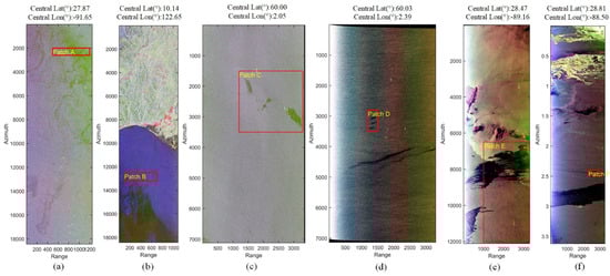
Figure 2.
Pauli RGB images of the study area: (a) case 1; (b) case 2; (c) case 3; (d) case 4; (e) case 5; (f) case 6.
3.2. Evaluation Indicators
To evaluate the advantage of the for oil spill detection, we used two common metrics for evaluating oil–water separation. In previous studies, various contrast ratios have been developed and improved to evaluate detector performance. Michelson Contrast (MC) has been used to quantitatively evaluate the distinguishability of seawater and oil slicks [19,32]. Its definition formula is as follows:
where and represent the maximum and minimum average polarimetric eigenvalues between the two target samples under test, respectively, and the range of MC value is 0–1.
The Jeffries–Matusita (JM) distance can be used as a reliable factor for the detection of oil–water separability [18,33,34]. In [35], the JM distance between two classes, and , which are members of a set of C classes (I, j = 1, 2,…, C, i ≠ j), is defined as:
and represent the mean value, and and represent the covariance matrix of classes and . The value range of the JM distance is 0–2. The larger the JM distance, the higher the distinguishability between the two types of objects, and vice versa. When the JM distance is greater than 1.9, it indicates that the two target categories are highly distinguishable; when the JM distance is 1–1.9, it indicates that the two categories have good distinguishability; and when the JM distance is 0–1, it indicates that the distinguishability is weak [18,19].
3.3. Effectiveness Validation of Detector
The CP SAR data in this study was extracted from the FP SAR data. The Stokes vector of CP SAR can be obtained by Equations (4) and (5), and the child parameters can be extracted through the Stokes vector to obtain the polarimetric features in [19].
Figure 3 shows the Span results of the oil spill area in two ALOS images. Because the oil inhibits the backscattering of the sea surface, the brightness value of some areas on the SAR image decreases, and dark spots are formed. At the same time, it can also be seen that the dark spots are deep and shallow (red box area and blue box area), which depends on the thickness of the oil slick. Based on this, oil spill detection is divided into three categories: thick oil, thin oil and seawater.
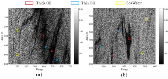
Figure 3.
Span image of oil spill at sea: (a) Case 1; (b) Case 2.
We can see the Span images of oil slicks in RADARSAT-2 and UAVSAR from Figure 4. The oil slicks in Figure 4a are, from left to right, plant oil (blue box), emulsion (orange box), and crude oil (red box). Figure 4b contains four films, including three different emulsions and one plant oil. The emulsions were all based on Troll and Oseberg crude oils, but the oil volume fractions were 80% oil (E80), 60% oil (E60) and 40% oil (E40), respectively. The plant oil is Radiagreen ebo, used to simulate a biological oil slick.
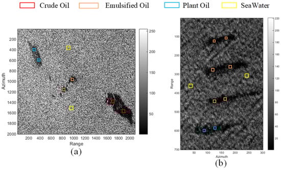
Figure 4.
Span image of oil spill at sea: (a) Case 3; (b) Case 4.
In Figure 5, the Span images of a large oil slick (Figure 5a) and a small oil slick (Figure 5b) are shown. The selection of these two study areas is to verify the edge extraction ability of the detector proposed in this paper for large and small patches. In Figure 5a, the red boxed areas are the main large oil slick areas, and the blue boxed area below is the splashed dispersant. Figure 5b shows small feathery oil slicks.
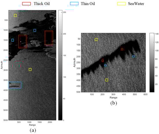
Figure 5.
Span image of oil spill at sea: (a) Case 5; (b) Case 6.
To confirm the validity of , we compare the results of with the other five polarimetric features. The polarimetric characteristic parameters mainly include three types: backscattered energy, correlation of different channels and scattering mechanisms. We selected some polarimetric features from each type for evaluating the effectiveness of . These five features have been widely used in oil slick detection by researchers: [13] and [15] mainly reflect the backscattered energy; [19] represents the correlation of different channels; DoP and [6] represent scattering mechanisms. The polarimetric features used for evaluation were selected from three directions, so it is more comprehensive and reasonable. Table 2 lists the five polarimetric features’ definition formulas compared with in this study, and their expected behavior for oil slicks and seawater. In the table, , is the i-th eigenvalue.
Table 2.
Defining formulas for the five polarimetric characteristics and their expected behavior for oil slicks and seawater.
Figure 6 shows the visualization results of and five other parameters in the Gulf of Mexico for Case 1. From the figure, it can be analyzed that DoP, , and cannot clearly display the strip-like thin oil area on the left and the middle. Although the polarimetric feature maps of and are better than DoP in terms of contrast, there is a small missed detection in the thick oil region. If the two are combined into , then after information superposition, the advantages of both can be combined, and the shortcomings of missed detection can be discarded. The detection of thick and thin oils by will be more complete and more effective.
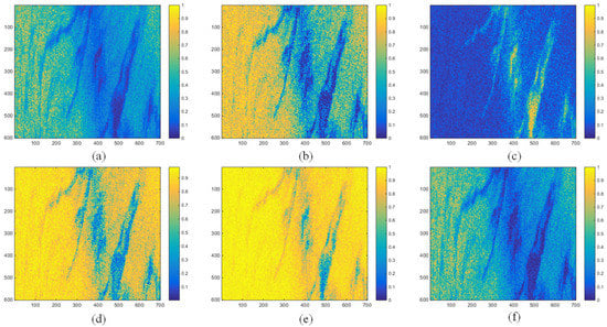
Figure 6.
Visualization results of different polarimetric features in Case 1: (a) ; (b) ; (c) ; (d) DoP; (e) ; (f) .
In Figure 7, we can see the visualization results of and five other parameters in Case 2. It can be analyzed from the figure: although the feature map of DoP can obviously extract the thick oil, the display of the thin oil area in the lower left corner is not obvious. and detectors are not good for the extraction of thin oil. The polarimetric feature map of is not clear for the extraction boundary of strip-like thick oil and block-like thick oil in the middle part. The and detectors can not only clearly extract thick oil, but also display the thin oil area.
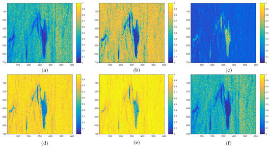
Figure 7.
Visualization results of different polarimetric features in Case 2: (a) ; (b) ; (c) ; (d) DoP; (e) ; (f) .
Figure 8 shows the visualization of and five other parameters in Case 3. We can see that the distinction between emulsion and crude oil is not obvious, and plant oil and crude oil are more distinguishable. DoP, and were weaker than the other three detectors in the extraction of plant oil.
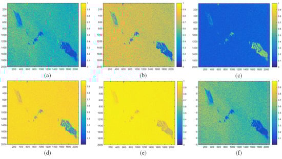
Figure 8.
Visualization results of different polarimetric features in Case 3: (a) ; (b) ; (c) ; (d) DoP; (e) ; (f) .
Figure 9 shows the feature extraction maps of emulsions and plant oils of different concentrations of crude oil in Case 4. The four detectors, except and detectors, are not very clear for the distinction between emulsions and plant oil. This shows that the backscattering energy has a good ability to identify and distinguish, and also shows that the detector can make up for the deficiency of the scattering mechanism and be more widely used in oil spill detection in various scenarios.
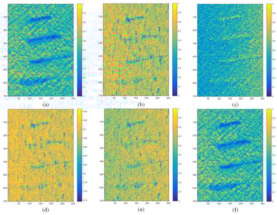
Figure 9.
Visualization results of different polarimetric features in Case 4: (a) ; (b) ; (c) ; (d) DoP; (e) ; (f) .
The polarimetric feature extraction map of the large oil slick in Case 5 can be seen in Figure 10. Although all detectors can display the main two oil slicks, the feature extraction maps of , DoP, and are not completely extracted for the nearby thin oil. Compared with the detector, the detector has a more obvious distinction between thick oil and thin oil, and the contrast is stronger.
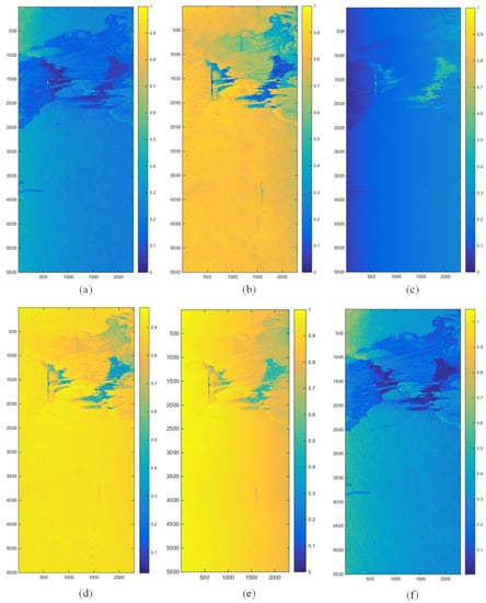
Figure 10.
Visualization results of different polarimetric features in Case 5: (a) ; (b) ; (c) ; (d) DoP; (e) ; (f) .
The small oil slick in Case 6 can be seen in Figure 11. The five feature maps except can clearly identify the edge of the feather-like oil slick, and the contrast between the and detector is more obvious and have better distinguishability.

Figure 11.
Visualization results of different polarimetric features in Case 6: (a) ; (b) ; (c) ; (d) DoP; (e) ; (f) .
Figure 12 shows the MC measurement results for the six polarimetric features studied in the case. It shows the ranking results between oil slick thickness (a), (b), different types of oil slicks (c), (d), (e), and different sizes of oil slicks (f), (g). Overall, the detector can distinguish different oil spill scenarios well and outperform the other five detectors in most cases, because it is a combination of two polarimetric features, and it can enhance the information from both backscattering energy and scattering mechanisms. Therefore, the distinguishability is better. The and parameters also have better discriminative ability, but they are not as good as in general.
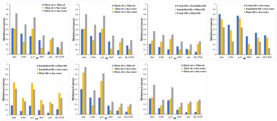
Figure 12.
MC measurement results: (a) Case 1; (b) Case 2; (c,d) Case 3; (e) Case 4; (f) Case 5; (g) Case 6.
Figure 13 shows the JM distance assessment results for the study area. The JM distance can reflect the distinguishability between two target categories, and if the JM distance is greater than 1.9, it means that the two have strong distinguishability. From the results, the detector has a good effect on the thickness inspection of oil slicks and oil slicks of different sizes. In different types of oil slick detection, the distinction between crude oil and emulsion is not ideal. Overall, in most of the class comparisons, the JM distance of the detector is greater than 1.9, proving that it can highlight the oil slick signal by itself and suppress other similarities. Combined with the Michelson Contrast, the performance superiority of the detector can be fully demonstrated. This shows that the parameter of the PE decomposition is feasible and effective in oil spill detection.
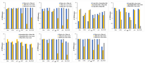
Figure 13.
JM distance measurement results: (a) Case 1; (b) Case 2; (c,d) Case 3; (e) Case 4; (f) Case 5; (g) Case 6.
3.4. Comparison of Classification Results
Variable importance is a parameter that evaluates how much each factor contributes to the classification result. After we extracted the feature maps of study area using the , we performed random forest classification on the feature maps.
Figure 14 and Figure 15 show the classification of oil slicks with different thicknesses and their respective variable importance rankings in Case 1 and Case 2, respectively. Table 3 and Table 4 show the respective producer and user accuracy results. The kappa coefficient can be used to evaluate classification accuracy [19]. It can be seen from the classification results that the distinction between the thin oil film and seawater in the right half of the figure does not have strict boundaries, but the classification and detection of thick oil films and seawater are accurate. According to the ranking results of variable importance, the contribution of is the largest, followed by , which proves the superiority of the detector in the detection of oil films with different thicknesses.
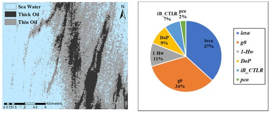
Figure 14.
Random forest classification result graph and variable importance ranking for Case 1.
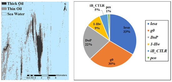
Figure 15.
Random forest classification result graph and variable importance ranking for Case 2.
Table 3.
Classification accuracies of random forest classifier in Case 1.
Table 4.
Classification accuracies of random forest classifier in Case 2.
Figure 16 and Figure 17 show the classification and variable importance ranking of different types of oil films in Case 3 and Case 4. Table 5 and Table 6 show the respective producer and user accuracy results. It can be seen from Case 3 that the thicker emulsion is classified as crude oil, and the thin oil films around the emulsions and crude oil are classified as plant oil. The contribution of and is the highest among all detectors, and their performance is close. Likewise, the thin oil film of the emulsion in Case 4 was classified as plant oil, while the thicker part of plant oil was incorrectly classified as emulsions. The contribution of was the highest among the six detectors.
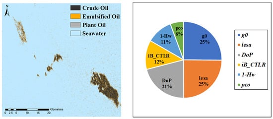
Figure 16.
Random forest classification result graph and variable importance ranking for Case 3.
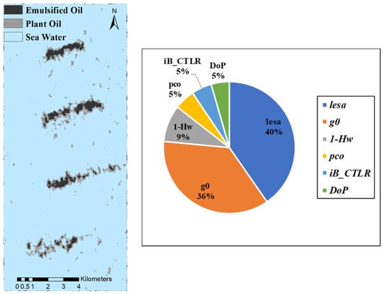
Figure 17.
Random forest classification result graph and variable importance ranking for Case 4.
Table 5.
Classification accuracies of random forest classifier in Case 3.
Table 6.
Classification accuracies of random forest classifier in Case 4.
Figure 18 and Figure 19 show the classification and variable importance ranking of oil films with different sizes in Case 5 and Case 6. Table 7 and Table 8 show the respective producer and user accuracy results. From the classification results, it can be seen that for large oil slicks, can accurately identify the two main oil spill areas, as well as the surrounding thin oil areas and the splashing dispersant below, but there is a misclassification of seawater as thin oil. Among the six polarimetric features, has the highest contribution, followed by . For a small oil slick, the detection results are also relatively good, among which has the highest contribution, followed by .
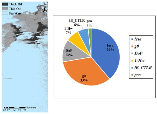
Figure 18.
Random forest classification result graph and variable importance ranking for Case 5.
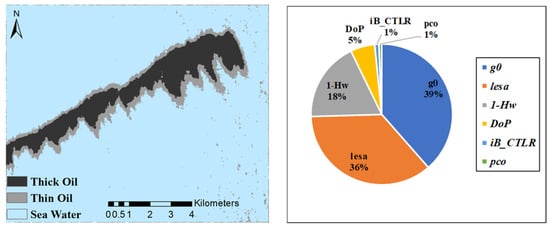
Figure 19.
Random forest classification result graph and variable importance ranking for Case 6.
Table 7.
Classification accuracies of random forest classifier in Case 5.
Table 8.
Classification accuracies of random forest classifier in Case 6.
The kappa accuracy of random forest classification for six polarized features in six cases are shown in Figure 20. Among them, the Kappa accuracy of is dominant in all five cases. This proves the point of this study that the detector can combine the advantages of scattering mechanism and backscattering energy to perform more accurate detection of oil slicks through information enhancement.
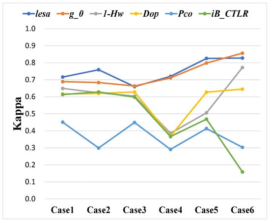
Figure 20.
Kappa accuracy of random forest classification for six polarized features in six cases.
4. Conclusions
The PE decomposition was originally proposed for ship detection. This study innovatively uses the PE decomposition for oil spill detection and proves that can clearly extract oil slicks. The main outcomes are summarized as follows:
- For oil spill detection using CP SAR data, the parameters of PE decomposition are introduced in this paper. Based on the PE decomposition, the parameter can be obtained as a detector to extract features. The parameter combines two conventional detectors: entropy () and total scattering power (), thereby enhancing the contrast between oil slicks and seawater. Experiments were carried out on six representative scenes, and the separability of target categories was quantitatively assessed using Michelson contrast and Jeffries–Matusita distance on feature maps. The evaluation results show that the MC measurement results of is superior in most scenarios, and the JM distance measurement results are mostly greater than 1.9. Finally, random forest classification was performed, and the classification accuracy has advantages in all five scenarios. The evaluation results demonstrate the superiority of the parameters of the PE decomposition for oil spill detection.
- Based on three categories, including different thickness of oil films, different types of oil films and different sizes of oil films, we evaluated the performance and superiority of the . Compared with other types of polarimetric characteristic parameters, the can overcome some of the shortcomings of entropy () and total scattered power (), and combine the information of both. This helps to improve the extraction of oil slick information, thereby making oil spill detection more accurate.
From the current research, the PE decomposition has been successfully applied to ship detection and oil spill detection, and the results obtained are also satisfactory. This study only verifies the effectiveness of from the perspective of polarimetric characteristics. Moreover, is verified to be feasible by using the representative random forest classification method, which is widely used. However, further investigation is needed to determine whether this advantage is specific to random forest classification and whether the above conclusions still hold with other machine learning algorithms. At present, this work has not been done, and there may be some challenges. For example, in deep learning methods, how to design networks adapted to and compact polarimetric situations still needs further discussion and in-depth investigation in the future.
Author Contributions
Conceptualization, S.G.; methodology, H.L.; writing—original draft preparation, S.L.; writing—review and editing, S.L.; supervision, H.L. All authors have read and agreed to the published version of the manuscript.
Funding
This work was supported in part by the National Nature Science Foundation of China under Grant 62173133, in part by Nature Science Foundation of Hunan Province 2020JJ4213, in part by Fundamental Research Funds for the Central Universities under Projects 2682020ZT34 and 2682021CX071, in part by the CAST Innovation Foundation, and in part by the State Key Laboratory of Geo-Information Engineering under Projects SKLGIE2020-Z-3-1 and SKLGIE2020-M-4-1.
Data Availability Statement
Not applicable.
Conflicts of Interest
The authors declare no conflict of interest.
References
- Buono, A.; Nunziata, F.; Migliaccio, M.; Li, X. Polarimetric Analysis of Compact-Polarimetry SAR Architectures for Sea Oil Slick Observation. IEEE Trans. Geosci. Remote Sens. 2016, 54, 5862–5874. [Google Scholar] [CrossRef]
- Lupidi, A.; Staglianò, D.; Martorella, M.; Berizzi, F. Fast Detection of Oil Spills and Ships Using SAR Images. Remote Sens. 2017, 9, 230. [Google Scholar] [CrossRef]
- Yang, J.; Ma, Y.; Hu, Y.; Jiang, Z.; Zhang, J.; Wan, J.; Li, Z. Decision Fusion of Deep Learning and Shallow Learning for Marine Oil Spill Detection. Remote Sens. 2022, 14, 666. [Google Scholar] [CrossRef]
- Salberg, A.-B.; Rudjord, Ø.; Solberg, A.H.S. Oil Spill Detection in Hybrid-Polarimetric SAR Images. IEEE Trans. Geosci. Remote Sens. 2014, 52, 6521–6533. [Google Scholar] [CrossRef]
- Charbonneau, F.J.; Brisco, B.; Raney, R.K.; McNairn, H.; Liu, C.; Vachon, P.W.; Shang, J.; DeAbreu, R.; Champagne, C.; Merzouki, A.; et al. Compact polarimetry overview and applications assessment. Can. J. Remote Sens. 2010, 36, S298–S315. [Google Scholar] [CrossRef]
- Nunziata, F.; Migliaccio, M.; Li, X. Sea Oil Slick Observation Using Hybrid-Polarity SAR Architecture. IEEE J. Oceanic Eng. 2015, 40, 426–440. [Google Scholar] [CrossRef]
- Li, Y.; Zhang, Y.; Chen, J.; Zhang, H. Improved Compact Polarimetric SAR Quad-Pol Reconstruction Algorithm for Oil Spill Detection. IEEE Geosci. Remote Sens. Lett. 2014, 11, 1139–1142. [Google Scholar] [CrossRef]
- Souyris, J.-C.; Imbo, P.; Fjortoft, R.; Mingot, S.; Lee, J.-S. Compact polarimetry based on symmetry properties of geophysical media: The π/4 mode. IEEE Trans. Geosci. Remote Sens. 2005, 43, 634–646. [Google Scholar] [CrossRef]
- Stacy, N.; Preiss, M. Compact polarimetric analysis of X-band SAR data. In Proceedings of the EUSAR 2006—6th European Conference on Synthetic Aperture, Dresden, Germany, 16–18 May 2006. [Google Scholar]
- Nord, M.E.; Ainsworth, T.L.; Lee, J.-S.; Stacy, N.J.S. Comparison of Compact Polarimetric Synthetic Aperture Radar Modes. IEEE Trans. Geosci. Remote Sens. 2009, 47, 174–188. [Google Scholar] [CrossRef]
- Raney, R.K. Hybrid-Polarity SAR Architecture. IEEE Trans. Geosci. Remote Sens. 2007, 45, 3397–3404. [Google Scholar] [CrossRef]
- Yin, J.; Yang, J.; Zhou, L.; Xu, L. Oil Spill Discrimination by Using General Compact Polarimetric SAR Features. Remote Sens. 2020, 12, 479. [Google Scholar] [CrossRef]
- Liu, P.; Li, X.; Qu, J.; Wang, W.; Zhao, C.; Pichel, W. Oil spill detection with fully polarimetric UAVSAR data. Mar. Pollut. Bull. 2011, 62, 2611–2618. [Google Scholar] [CrossRef]
- Shirvany, R.; Chabert, M.; Tourneret, J.-Y. Ship and Oil-Spill Detection Using the Degree of Polarization in Linear and Hybrid/Compact Dual-Pol SAR. IEEE J. Sel. Top. Appl. Earth Obs. Remote Sens. 2012, 5, 885–892. [Google Scholar] [CrossRef]
- Yin, J.J.; Yang, J.; Zhou, Z. New parameters in compact polarimetry for ocean target detection. In Proceedings of the IET International Radar Conference 2013, Xi’an, China, 14–16 April 2013. [Google Scholar]
- Yin, J.; Yang, J.; Zhou, Z.-S.; Song, J. The Extended Bragg Scattering Model-Based Method for Ship and Oil-Spill Observation Using Compact Polarimetric SAR. IEEE J. Sel. Top. Appl. Earth Obs. Remote Sens. 2015, 8, 3760–3772. [Google Scholar] [CrossRef]
- Singha, S.; Ressel, R. Offshore platform sourced pollution monitoring using space-borne fully polarimetric C and X band synthetic aperture radar. Mar. Pollut. Bull. 2016, 112, 327–340. [Google Scholar] [CrossRef]
- Tong, S.; Liu, X.; Chen, Q.; Zhang, Z.; Xie, G. Multi-Feature Based Ocean Oil Spill Detection for Polarimetric SAR Data Using Random Forest and the Self-Similarity Parameter. Remote Sens. 2019, 11, 451. [Google Scholar] [CrossRef]
- Li, G.; Li, Y.; Hou, Y.; Wang, X.; Wang, L. Marine Oil Slick Detection Using Improved Polarimetric Feature Parameters Based on Polarimetric Synthetic Aperture Radar Data. Remote Sens. 2021, 13, 1607. [Google Scholar] [CrossRef]
- Krestenitis, M.; Orfanidis, G.; Ioannidis, K.; Avgerinakis, K.; Vrochidis, S.; Kompatsiaris, I. Oil Spill Identification from Satellite Images Using Deep Neural Networks. Remote Sens. 2019, 11, 1762. [Google Scholar] [CrossRef]
- Li, Y.; Lyu, X.; Frery, A.C.; Ren, P. Oil Spill Detection with Multiscale Conditional Adversarial Networks with Small-Data Training. Remote Sens. 2021, 13, 2378. [Google Scholar] [CrossRef]
- Gao, G.; Gao, S.; He, J.; Li, G. Adaptive Ship Detection in Hybrid-Polarimetric SAR Images Based on the Power–Entropy Decomposition. IEEE Trans. Geosci. Remote Sens. 2018, 56, 5394–5407. [Google Scholar] [CrossRef]
- Nunziata, F.; Gambardella, A.; Migliaccio, M. On the Mueller Scattering Matrix for SAR Sea Oil Slick Observation. IEEE Geosci. Remote Sens. Lett. 2008, 5, 691–695. [Google Scholar] [CrossRef]
- Nunziata, F.; Sobieski, P.; Migliaccio, M. The Two-Scale BPM Scattering Model for Sea Biogenic Slicks Contrast. IEEE Trans. Geosci. Remote Sens. 2009, 47, 1949–1956. [Google Scholar] [CrossRef]
- Raney, R.K. Dual-polarized SAR and Stokes parameters. IEEE Geosci. Remote Sens. Lett. 2006, 3, 317–319. [Google Scholar] [CrossRef]
- Cloude, S.R. Polarisation: Applications in Remote Sensing; Oxford University Press: London, UK, 2009. [Google Scholar]
- Kim, D.; Moon, W.M.; Kim, Y. Application of TerraSAR-X Data for Emergent Oil-Spill Monitoring. IEEE Trans. Geosci. Remote Sens. 2010, 48, 852–863. [Google Scholar]
- Breiman, L. Random forests. Mach. Learn. 2001, 45, 5–32. [Google Scholar] [CrossRef]
- Pal, M. Random Forest classifier for remote sensing classification. Int. J. Remote Sens. 2005, 26, 217–222. [Google Scholar] [CrossRef]
- Conceição, M.R.A.; de Mendonça, L.F.F.; Lentini, C.A.D.; da Cunha Lima, A.T.; Lopes, J.M.; de Vasconcelos, R.N.; Gouveia, M.B.; Porsani, M.J. SAR Oil Spill Detection System through Random Forest Classifiers. Remote Sens. 2021, 13, 2044. [Google Scholar] [CrossRef]
- Migliaccio, M.; Gambardella, A.; Nunziata, F.; Shimada, M.; Isoguchi, O. The PALSAR Polarimetric Mode for Sea Oil Slick Observation. IEEE Trans. Geosci. Remote Sens. 2009, 47, 4032–4041. [Google Scholar] [CrossRef]
- Skrunes, S.; Brekke, C.; Eltoft, T. Characterization of Marine Surface Slicks by Radarsat-2 Multipolarization Features. IEEE Trans. Geosci. Remote Sens. 2014, 52, 5302–5319. [Google Scholar] [CrossRef]
- Dabboor, M.; Howell, S.; Shokr, M.; Yackel, J. The Jeffries–Matusita distance for the case of complex Wishart distribution as a separability criterion for fully polarimetric SAR data. Int. J. Remote Sens. 2014, 35, 6859–6873. [Google Scholar]
- Li, G.; Li, Y.; Liu, B.; Wu, P.; Chen, C. Marine Oil Slick Detection Based on Multi-Polarimetric Features Matching Method Using Polarimetric Synthetic Aperture Radar Data. Sensor 2019, 19, 5176. [Google Scholar] [CrossRef] [PubMed]
- Swain, P.H.; Davis, S.M. Remote Sensing: The Quantitative Approach; McGraw-Hill: New York, NY, USA, 1978. [Google Scholar]
Publisher’s Note: MDPI stays neutral with regard to jurisdictional claims in published maps and institutional affiliations. |
© 2022 by the authors. Licensee MDPI, Basel, Switzerland. This article is an open access article distributed under the terms and conditions of the Creative Commons Attribution (CC BY) license (https://creativecommons.org/licenses/by/4.0/).