Abstract
Remote monitoring of natural afforestation processes on abandoned agricultural lands is crucial for assessments and predictions of forest cover dynamics, biodiversity, ecosystem functions and services. In this work, we built on the general approach of combining satellite and field data for forest mapping and developed a simple and robust method for afforestation dynamics assessment. This method is based on Landsat imagery and index-based thresholding and specifically targets suitability for limited field data. We demonstrated method’s details and performance by conducting a case study for two bordering districts of Rudnya (Smolensk region, Russia) and Liozno (Vitebsk region, Belarus). This study area was selected because of the striking differences in the development of the agrarian sectors of these countries during the post-Soviet period (1991-present day). We used Landsat data to generate a consistent time series of five-year cloud-free multispectral composite images for the 1985–2020 period via the Google Earth Engine. Three spectral indices, each specifically designed for either forest, water or bare soil identification, were used for forest cover and arable land mapping. Threshold values for indices classification were both determined and verified based on field data and additional samples obtained by visual interpretation of very high-resolution satellite imagery. The developed approach was applied over the full Landsat time series to quantify 35-year afforestation dynamics over the study area. About 32% of initial arable lands and grasslands in the Russian district were afforested by the end of considered period, while the agricultural lands in Belarus’ district decreased only by around 5%. Obtained results are in the good agreement with the previous studies dedicated to the agricultural lands abandonment in the Eastern Europe region. The proposed method could be further developed into a general universally applicable technique for forest cover mapping in different growing conditions at local and regional spatial levels.
1. Introduction
The phenomenon of abandonment of agricultural lands has been observed and studied all over the world for many years [1,2,3,4]. Such processes also manifested across the entire post-Soviet space, including Russia and the Republic of Belarus [5]. After the collapse of the Soviet Union, the economic developments of these two neighbouring countries have followed different pathways. This divergence has dramatically affected conditions of initially very similar agricultural sectors, leading to different dynamics of the areas under cultivation [6].
Existing literature features a variety of methods for the assessment of abandoned agricultural land areas that have naturally afforested at different spatial scales. Goga et al. (2019) presented a detailed overview of such methods and satellite data used around the world, including Central and Eastern Europe, with an aim to identify abandoned agricultural lands [7]. Time series of Landsat and Moderate Resolution Imaging Spectroradiometer (MODIS) satellite data have been used to identify and map land abandonment [8,9]. Combined mapping techniques have been applied at the level of entire countries to create hybrid maps of arable and abandoned lands [10,11]. In Russia, Landsat data are often used for local and regional assessments due to the availability of lengthy time series [12,13].
In our current work, we are less interested in the fact of abandoning agricultural lands and more interested in the young forests developed due to the natural afforestation of these lands. Reliable information about the afforestation of agricultural lands in Russia has become especially important for the planning, implementation and monitoring of new local climate projects related to international and national climate change resolutions and programs [14,15,16]. In addition, such information on newly developed forests is essential for studying their biodiversity, ecosystem services, carbon sequestration, novel ecosystems, etc. [17,18,19].
According to the definition given by Food and Agriculture Organization of the United Nations (FAO) [20], the term “afforestation” corresponds exclusively to the establishment of forest through planting and/or deliberate seeding. Alternatively, the term “natural expansion of forest” is defined as an expansion of forest through natural succession. In this paper we focus specifically on natural forest expansion, but for the sake of wording simplicity we refer to this process as “natural afforestation” or simply “afforestation”.
Satellite data can be used to assess the spatial dynamics of forest cover. Various methods for time series analysis of satellite images have been developed to map forests and other ecosystems. Supervised classification with a data-learned model requires a representative dataset of training samples for all land cover types captured in the image [21,22], even if the aim is to produce a binary map (e.g., forest/non-forest discrimination). In contrast, threshold classification of spectral indices can be a simpler solution for specific cases, especially given the limited available ground-truth data [23]. Arable lands dynamics mapping can be conducted based on different vegetation indices (PVI, SAVI, etc.) that are derived from visible and near-infrared (NIR) bands of MODIS time series [24,25]. The choice of frequent but limited-resolution MODIS observations is governed due to the high variability of vegetation conditions on agricultural lands throughout a year. However, such methods are difficult to apply for Landsat data because of the low observation frequency of this satellite system. Computationally intensive methods, based on modelling of the annual dynamics of field’s reflectance, are required to implement “MODIS-like” processing scheme on Landsat imagery [26,27].
Compared to agricultural lands, forests are more stable and inertial ecosystems throughout the growing season, as the natural afforestation process can take decades. Therefore, the spatial dynamics of forest cover can be monitored by assessing spectral indices less often. Both classic indices [28] and new combinations [29,30] of spectral bands can be used for forest cover assessments. Lehmann et al. used a simple linear combination of Landsat’s red and NIR bands to study Australia’s forest cover trend at the national level [29]. Wentao Ye et al. have proposed a forest index based on three visible and NIR bands, which use tuneable thresholds [30]. This index requires an empirical set of green and NIR coefficients for the local area, as well as atmospherically calibrated Landsat data. However, there are still some challenges in forest cover discrimination from other land cover types. Dense forest stands can be misclassified with dark water bodies by using vegetation indices that are based only on visible and NIR spectral bands [31]. Therefore, it is necessary to mask-out such objects in the images in advance. Acharya et al. tested several indices for water bodies identification [31]. The modified normalized difference water index (MNDWI) allows for a more confident spectral separation of water from forest areas [32]. Additionally, in case of agricultural lands afforestation, it is important to find a solution for reliable discrimination between young forest and surrounding non-tree vegetation, since the abandoned fields are initially transformed into grasslands before the first trees appear. Becker et al. proposed an index that is stated to be suitable for such a problem [33].
Therefore, the primary aim of our study was to develop a relatively simple and robust method to assess the spatial dynamics of forest cover on abandoned agricultural lands, based on Landsat time series analysis and limited field data. Additionally, to evaluate the efficiency of the developed method, we performed a comparative analysis of natural afforestation dynamics in two bordering regions of Russia and the Republic of Belarus over the past 35 years.
2. Materials and Methods
2.1. Study Area
The Rudnya district in the Smolensk region of the Russian Federation and The Liozno district in the Vitebsk region of the Republic of Belarus were chosen as model areas for our study (Figure 1).
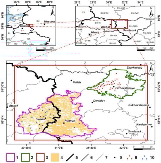
Figure 1.
Study area. Legend: 1—Rudnya and Liozno districts borders; 2—Smolenskoe Poozerie National Park border; 3—Extended study area for Landsat mosaics generation; 4—Initial Agricultural Lands (IAL); 5—Russia and Belarus state border; 6–Smolensk and Vitebsk regions borders; 7—Other state and administrative borders; 8—Populated places; 9—Field plots; 10—Visually identified bare soil plots. Nearby located plots are depicted by single marker. Countries and regions are marked with ISO 3166 codes.
Both districts are located in the subzone of coniferous–deciduous forests [34] and have similar climatic and soil conditions [35]. The climate is temperate continental and the average annual temperature is 7.5 °C. The highest monthly averaged temperature is +19.4 °C (in July) and the lowest one is −6.4 °C (in January). The average annual precipitation is 650 mm and the duration of the growing season (at temperatures above +10 °C) is 152 days [36,37]. Sod-podzolic soils prevail in the study area.
Besides two districts, we used observation data of vegetation plots collected in the National Park (NP) “Smolenskoe Poozerie” (Demidov district of the Smolensk region) in 2006–2019 (Figure 1). The NP is located close to the model territory (the minimum distance from the northern border of the Rudnya district to the border of the NP is 15 km) and exhibits no noticeable differences in terms of climatic and soils conditions. Since both districts and the NP are located close to each other, thematic processing of satellite data was carried out for a single rectangular footprint (extended study area) that covers all its territories simultaneously (Figure 1). However, forest cover dynamics analysis was conducted only for the study area of two bordering districts. Up-to-date characteristics for all three distinct regions within the extended study area, acquired via corresponding official web-sources [38,39,40,41,42,43,44], are provided in Table 1. We specifically stress that this official statistical information does not count any afforested agricultural lands towards forest cover area, since their legal status has not yet been modified.

Table 1.
Main up-to-date characteristics of regions within the extended study area.
2.2. Materials
2.2.1. Mask of Initial Agricultural Lands
The first step of our research was to determine the initial territory of agricultural lands (IAL) within the study area and to generate its geospatial mask (Figure 1). We digitized the boundaries of non-forest lands of our model territory using topographic maps of the 1970–1980s in scale 1:100,000. Topographic objects, indicated on these maps with areal signs as forests, swamps, water bodies and settlements, were consequently excluded. The GIS calculated IAL mask areas of the Rudnya and Liozno districts were 1285.60 square kilometers (60.5%) and 726.30 square kilometers (52.1%), respectively.
2.2.2. Field Data
Geobotanical descriptions of grasslands and young forests (up to 30 years old) on abandoned agricultural lands in the NP “Smolenskoe Poozerie” were carried out on square plots with a side length of 20 m in 2006–2019 [45]. On the plots, vegetation type and species composition of vascular plants and mosses were determined with an assessment of the projective cover of each species, taking into account the layer structure of the community.
In our study, we used 263 plots, of which 123 were forests and 140–grasslands (Figure 1). Geographic coordinates of the plots are given in Table S1 of the Supplementary Materials.
2.2.3. Landsat Data
Surface reflectance (SR) image data [46] derived from the Tier 1 scenes of Landsat Collection 1 [47] was used for the generation of multi-temporal image composites (mosaics) over the extended study area, which intersected six tiles of the Landsat Worldwide Reference System-2 [48] at paths 181–183 and rows 21, 22. All available relevant scenes for the years 1984–2020 by Landsat 4, 5, 7 and 8 satellites were incorporated in geo-processing, except Landsat 7 SLC-off images (acquired after 31 May 2003) due to its “striping” issues [49]. Initial Landsat SR data (741 scenes totally) were accessed and further processed to mosaics via the Google Earth Engine (GEE) platform [50]. Landsat images acquired by satellites with different sensors have unequal sets of spectral bands with similar but not identical specifications, so the essential characteristics for the six common bands of the visual, near and short-wave infrared ranges, which were utilized in our study, are shown in Table 2.
Table 2.
Characteristics of utilized spectral bands of Landsat images acquired by different satellite sensors.
2.2.4. Auxiliary Data
Freely available vector layers from the OpenStreetMap (OSM) dataset [51] were used to correct thematic products derived from Landsat imagery by identifying and masking-out urban objects (built-up areas and road network) within the study area. Polygonal features of “Places” (populated places boundaries) and “Buildings” (separate buildings boundaries), and linear features of “Roads” and “Railways” for territories of Belarus and the Central Federal District of Russia were acquired via Geofabrik Downloads [52]. The layers utilized in our study contained OSM data up to the end of April 2020.
2.3. Methods
For a more detailed analysis of the forest cover dynamics within the IAL, the corresponding mask was stratified into two landcover classes: arable lands and grasslands. We considered the “bare soil” spectral signature as an indicator of arable lands. However, since the periodicity of Landsat observations does not allow to sufficiently frequently monitor the “bare soil” pixels throughout the whole year, we decided to create an integral product for all years. We called this product “arable lands”, i.e., where bare soil pixel was detected at least once during the entire observation period. The remaining pixels, which never indicated bare soil presence over the 35 years, were labelled as “grasslands” class and included non-forest (non-tree) vegetation (grass, shrub, etc.).
Figure 2 shows a flowchart of satellite, field and auxiliary data processing methods used in our study. Cloudless Landsat mosaics were generated via GEE (Section 2.3.1) and harmonized for further thematic processing (Section 2.3.2). Three spectral indices, each specifically designed for either forest, water or bare soil identification, were used for forest cover and arable lands mapping (Section 2.3.3). We used field data of 2006–2010 to identify a threshold for forest cover masking (Section 2.3.4). A visual interpretation of very high-resolution satellite images and ground-based grassland plots of 2006–2010 were used to identify a threshold for bare soil masking (Section 2.3.5). The accuracy assessment of forest and bare soil masking was performed based on field plots collected during 2016–2020 (Section 2.3.6). Additional thematic masks of water and urban objects was created (Section 2.3.7). All generated thematic products were combined together for afforestation dynamics assessment (Section 2.3.8 and Section 2.3.9).

Figure 2.
Flowchart of data processing methods used in the study.
2.3.1. Multi-Temporal Mosaics Generation
Two different sets of Landsat mosaics were generated. The first one contained eight composites, which were derived from scenes acquired within sequential five-year periods and utilized for forest cover mapping. Five-year periods were counted from 1981 to 2020 and were denoted by the last year of the interval: for example, scenes from 2016 to 2020 were used to compose a five-year mosaic marked as 2020, scenes from 2011 to 2015 were used for 2015, etc. There is no appropriate Landsat data over our study area for the year 2012 and before 1984, so the five-year mosaic for 2015 was actually a four-year composite, and only two years of observations were used for 1985. The second set of Landsat mosaics contained 36 annual composites for the years from 1984 to 2020 (excluding 2012) and were utilized for arable land identification.
Mosaics for both sets were composed in GEE using the widespread processing scheme [53], including the following automated routines: (1) Filtering of the satellite image collection by the area of interest boundary, acquisition time period and image properties; (2) Masking-out of cloud, cloud-shadow and saturated pixels for remaining images in the collection; (3) Reducing a masked image collection to a composite by applying an aggregate function to the overlapping pixels for every set of corresponding image bands. Within GEE, sets of SR images captured by different Landsat satellites are organized in different image collections. In our study we used a total of four GEE image collections (of Landsat 4, 5, 7 and 8 data, respectively) for mosaics generation. The boundary of the extended study area was utilized for collections’ spatial filtering, an acquisition period was limited to a five-month growing season from May 1 to September 31 (between 121 and 274 day of the year) and only images with a precomputed “CLOUD_COVER” property value less than 50% were used in further processing. The only differences between the annual and five-year mosaics filtering process were the start and end values in the acquisition year filter, which reduced the collection either to the single year stack of images, or to the five-sequential years stack, respectively. As Landsat SR products already contain precomputed per-pixel quality assessment bitmasks with information about cloud/cloud–shadow cover and radiometric saturation, they were utilized to mask-out invalid pixel values. The median function was used for reducing image stacks to a single composite, since it has proved to be a simple and reliable technique that effectively suppresses the occurrence of residual clouds, shadows, haze and artifacts of another source on the resulting mosaic [53]. If the temporal coverages of two collections overlapped for a particular composite (e.g., the Landsat 4 and Landsat 5 collections for the 1990 five-year mosaic), both collections were processed sequentially and merged together just before the median reduction.
The code of the GEE script used for Landsat mosaics generation is provided in the Supplementary Materials.
2.3.2. Mosaics Normalization
Both sets of five-year and annual mosaics were harmonized for further processing via normalization procedure in order to reduce dissimilarity of SR values obtained by different Landsat sensors. In our study, we used a normalization technique based on the pseudo-invariant features (PIF) concept [54]. The PIF-based normalization procedure usually consists of three main steps: (1) Calculating the pixel-wise similarity measure(s) between the reference image and the image to be normalized, and identifying pseudo-invariant pixels based on a pre-set similarity threshold; (2) Fitting a linear regression model to the paired values of pseudo-invariant pixels for each image band; (3) Applying the obtained linear models to all pixels in the corresponding bands of the to-be-normalized image. All mosaics generated in GEE have been normalized according to this scheme using a custom program script written in the R environment [55]. We utilized the raster package [56] functions for basic operations with image data and modified the pifMatch function from the RStoolbox package [57] to perform the normalization.
A combination of two similarity criterions was used for pseudo-invariant pixels identification (in contrast to the original pifMatch, that accepts only single criterion at once). The first criterion was a Pearson’s correlation coefficient r calculated at per-pixel level for vectors of per-band SR values from two matching images. The second criterion was a per-pixel difference d between SR values of the two matching images computed independently for each band. Generally, it is reasonable to assume that a low inter-band correlation between pixels of the two composites over different years may indicate qualitative changes in the land cover (e.g., deforestation), while a high difference in absolute SR values indicate quantitative ones (e.g., increasing of the tree stand density). Therefore, the closer the r-value is to one and the d-values for all bands to zero, the lower the probability of changes in a particular pixel, so it can be used as a PIF for image normalization.
In our study, pixels with an r-value over 0.995 and d-values lying within the upper or lower quartiles for each band’s distribution simultaneously were considered as pseudo-invariant. The threshold value for r and the interval width for d were selected empirically based on the resulting fraction of pseudo-invariant pixels in the reference image. The fraction of pixels satisfying these criteria varied within the range of 4–6% (around one million pixels) for most of the processed mosaics. A five-year composite for 2010 was selected as a reference image, since the majority of field data were collected during the 2006–2010 period.
Generalized additive models (GAM) were fitted for prediction of normalized values using the bam function of the mgcv package [58], instead of the simple linear models (LM) utilized in the pifMatch. According to our experiments, GAM provided better normalization results in terms of model goodness of fit metrics (coefficient of determination and root-mean-square error) and resulting image homogeneity, as LM-normalized mosaics are more prone to present sparsely distributed pixels with abnormal SR values.
More details about the program functions used, their settings and application context can be found in the code of the normalization script provided in the Supplementary Materials.
2.3.3. Spectral Indices
A set of three spectral indices was utilized for forest cover and arable land discrimination on normalized Landsat mosaics.
The first one was a slightly modified version of Forest Cover Index (FCI) proposed by S. J. Becker with co-authors for WorldView-2 multispectral images [33]. Two versions of FCI were developed in Becker’s study, one based on red and red-edge spectral bands, and another one on red and near infrared bands. Both versions of the index were found to be robust for forest and non-forest vegetation cover discrimination on images acquired during the summer period. In our study, the second version of FCI was used, as Landsat sensors lack bands in the red edge spectrum region. Originally, this index was defined as a simple product of SR values in red and near infrared image bands. However, such a multiplication operation dramatically expands the range of FCI values, compared to the initial Landsat bands, where SR values are stored in an integer scale of 0–10,000. Therefore, in order to avoid this “stretching” effect and to preserve reasonable values range, we added a square root transform to the index formula:
where Red and NIR are Landsat bands described in Table 2. Generally, high FCI values correspond to non-forest vegetation, bare soil and urban areas, medium values to tree cover of various density, and low values to water bodies, dark dense forest and shadows (Figure 3a,b) [33].

Figure 3.
Fragments of the 2006–2010 (a,c) five-year mosaics (NIR-SWIR1-Red synthesis) over the study area and respective FCI (b) and the NDVISI values (d).
In addition to the FCI, commonly known Modified Normalized Difference Water Index (MNDWI) [32] was utilized for better discrimination of water bodies and dark dense forests. In the case of Landsat images, MNDWI is calculated as a normalized difference of SR values in green and first short-wave infrared bands:
where Green and SWIR1 are Landsat bands described in Table 2. MNDWI varies within [−1, 1] range, and values greater than zero usually correspond to pure water pixels, negative values near zero–to mixed pixels with various water fractions, and low negative values–to terrestrial ecosystems.
MNDWI = (Green − SWIR1)/(Green + SWIR1),
We developed a specific index aimed to improve the discrimination of field’s bare soil and grassland classes. It is represented by a combination of three visible and NIR bands. If we look at spectral reflectance curves of bare soil and vegetation (Figure 1-1) in Blasch [59], we can see that bare soil reflectance in visible bands is higher than vegetation reflectance. At the same time, vegetation reflectance in the NIR band is higher than for bare soil. Thus, if we sum up all visible (Blue, Green and Red) bands and calculate the normalized difference visible index (NDVISI), then the bare soil value shall be significantly lower than the vegetation index value. NDVISI has the following equation:
where
and Blue, Green, Red and NIR are Landsat bands described in Table 2. NDVISI varies within [–1, 1] range. Bare soil has negative or very small positive index values (Figure 3c,d). The Urban and Water objects had also lower index values than vegetation, but we were able to mask them at thematic products generation step (Section 2.3.8).
NDVISI = (VIS − NIR)/(VIS + NIR),
VIS = (Blue + Green + Red),
The FCI and MNDWI images were calculated for the five-year Landsat mosaics, while the NDVISI–for the annual ones.
2.3.4. FCI Threshold Identification
A constant threshold for forest and non-forest vegetation discrimination was determined based on the FCI image for the 2010 five-year mosaic and field data collected during the corresponding period.
We collected two sets of field sampling points for forest cover and grassland classes. Then, we extracted the FCI value in each sampling point from the 2010 five-year mosaic image. The threshold value of the index between two classes was chosen experimentally based on maximum value of the Cohen Kappa [60]. This means we consistently moved the threshold from low index values to high ones until the Kappa reached its maximum.
2.3.5. NDVISI Threshold Identification
We used the five-year NDVISI mosaic and field data for the period 2006–2010 to identify the threshold between bare soil and grassland classes. Two types of reference data were collected: (i) field sampling points and (ii) points acquired from satellite images. Sampling points for grassland class were selected from field observations database. The bare soil points were visually identified on a five-year mosaic image (2010). The location of the point on the field was controlled by a visual inspection of Google Earth Web images [61]. Geographic coordinates of the bare soil points are provided in Table S2 of the Supplementary Materials.
The threshold between two classes was determined by the integral minNDVISI image (2010). We created this product to maintain the maximum number of bare soil values in five years. The five-year 2010 index was created by selecting a minimum pixel value from five annual NDVISI images for a given time period (2006–2010). The five-year minimum NDVISI images for all other seven time periods were created by the same method.
Then, we extracted the NDVISI index value at each sampling point of bare soil and grasslands classes from the 2010 five-year minNDVISI mosaic image. The threshold value of the NDVISI between two classes was chosen based on the maximum value of the Cohen Kappa. The procedure of “bare soil-grassland” threshold fitting was the same as “forest-grassland” threshold approach.
2.3.6. Threshold Verification
An accuracy assessment was conducted to investigate the possibility of applying FCI and NDVISI thresholds for all eight five-year period index images.
Assessment of the FCI threshold for forest cover masking was conducted using the five-year FCI image and field data for the 2016–2020 period. First, we collected two sets of field control points for forest cover and grassland classes. Then, we extracted FCI value in each control point from 2020 five-year index image. Using the FCI threshold of 2010 (Section 2.3.5), the control points were classified into two classes. Then, we calculated the Cohen Kappa values to assess the method’s accuracy.
An assessment of the NDVISI threshold for bare soil masking was conducted in the same manner as the assessment of the FCI threshold. However, we used the five-year minNDVISI image, control points for grassland class from field observations database and the bare soil points visually identified on five-year mosaic image (2020). Geographic coordinates of the bare soil control points are provided in Table S2 of the Supplementary Materials.
2.3.7. Water and Urban Objects Masks Generation
Independent thematic masks of water and urban objects were generated to exclude these areas from further forest cover dynamics analysis.
The water objects mask was generated based on multi-temporal MNDWI images. First, separate masks for all five-year mosaics were obtained by applying a constant threshold to the corresponding images of the index. Pixels with MNDWI values over −0.075 were considered as water. This threshold was determined by visual analysis of water objects on the 2010 five-year composite along with its MNDWI image. Since Landsat mosaics were normalized before the indices computation, a constant threshold should provide similar results for all of them without the need for individual adjustment. While obtained multi-temporal masks were sufficiently consistent over areal water bodies (lakes, ponds, wide rivers), narrow rivers and streams exhibited spatially inconsistent missingness patterns. To avoid this mislabelling issue of water bodies marked as a forest cover by the FCI threshold, all multi-temporal water masks were combined into a single image by the simple merging of all identified water pixels from different periods together. The resulting mask was also expanded by a one-pixel-wide buffer in order to include spectrally heterogeneous pixels on the waterside.
The urban objects mask was generated by rasterizing OSM vector layers with Landsat spatial resolution (30 m). Only features labelled with classes “city”, “town”, “village” and “suburb” were included in the mask from the “Places” layer, while “Buildings” and “Railroads” layers were rasterized entirely. From the “Roads” layer, features labelled with classes “primary”, “primary_link”, “secondary”, “secondary_link”, “tertiary”, “trunk”, “trunk_link”, “track_grade1”, “track_grade2”, “service”, “pedestrian”, “residential” and “living_street” were selected, as they can be visually identified on Landsat imagery. After rasterization, all pixels originated from different OSM layers were combined into a single urban objects mask.
2.3.8. Forest Cover Products Generation
To analyse the forest cover dynamics over the study area, a set of eight sequential forest cover masks were generated based on multi-temporal FCI images.
First, independent masks for all five-year periods were obtained by applying the determined threshold to the corresponding FCI images. Pixels with values lower than the threshold were considered as a potential forest cover. These pixels were further filtered by exclusion of water and urban objects based on corresponding thematic masks and by a temporal consistency check. A particular forest cover pixel of a certain period was considered to be consistent if corresponding pixels from at least all preceding or all subsequent periods were also marked as forest cover. Inconsistent pixels were filtered from all masks except ones for the start (1981–1985) and end (2016–2020) periods of the analysed sequence, since they cannot be adequately checked in both temporal directions simultaneously.
Bare soil mask was generated from five-year NDVISI indices. These indices were collected from annual NDVISI images based on the minimum NDVISI value criteria for each pixel. Then, each pixel of the five-year image was compared with the NDVISI threshold (2006–2010). It was labelled as “bare soil” if the NDVISI index value was less than the identified threshold (Section 2.3.5). Five-year bare soil masks were combined into a single raster layer for the entire period of observations (1985–2020).
2.3.9. Assessment of Forest Cover Area Dynamics
The forest cover area dynamic was assessed both within the boundaries of the IAL mask and the administrative district. During previous processing steps, water and urban masks were excluded from the IAL mask, hence corresponding areas were not assessed.
In our first case, we assigned arable land from all pixels within the boundaries of the IAL using the bare soil raster mask. All other pixels of the IAL mask were assigned to the grassland class. Five-year forest cover masks were then intersected with arable lands and grasslands to spatially define the afforested arable lands and afforested grasslands.
In the second case, arable lands were assigned from pixels within the boundaries of the administrative district using a mask of bare soil raster mask. All other pixels of the administrative district mask were assigned to other lands. Five-year forest masks intersected with arable lands and other administrative district lands to define areas of forests, arable land, and others. This procedure was performed for each five-year period. The calculated areas of all tree classes were normalized by the area of the administrative district.
3. Results
3.1. Landsat Mosaics Generation and Normalization
A total of 44 multi-temporal Landsat mosaics were generated in our study—36 for annual and 8 for five-year periods. Formally, none of these composites contained pixels with missing data for the study area, but the number of clear measurements available for aggregation varied greatly depending on the observation period (Figure 4), which naturally affected the quality of the obtained mosaics.
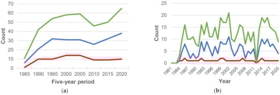
Figure 4.
Minimum (red), median (blue) and maximum (green) clear measurements per pixel count for generated Landsat mosaics over study area: (a) five-year composites; (b) annual composites.
Generally, the fewer measurements used for mosaic generation the higher the probability of artifacts occurrence and the lesser the homogeneity (seamlessness) of the resulting image. In our case, at least nine surface reflectance values per pixel were available during the five-year mosaic composition process (except 1981–1985 period, Figure 4a), but most of the generated annual mosaics (30 of 36) contained pixels with values derived from only one initial Landsat scene (Figure 4b). The recent five-year period of 2016–2020 contained the highest number of clear measurements—the median value count per pixel was 38 (with the maximum count of 65), and the early periods of 1981–1985 and 1986–1990, as might be expected, had the lowest number of cloudless observations with median counts of 6 (11) and 21 (42), respectively. For other five-year periods, median counts varied in the range of 26–32 (46–59). For the annual mosaics, these counts, naturally, were 3–5 times lower, so most of them were not completely continuous and seamless (Figure 5). Nevertheless, according to the visual analysis, only 8 obtained annual mosaics (namely, for years 1989, 1991, 1996, 2002, 2003, 2013, 2017, 2020) were of completely unsatisfactory quality and, therefore, were excluded from further processing.
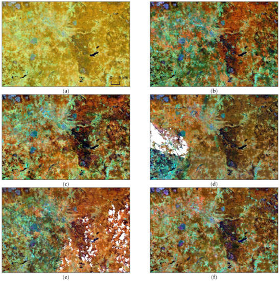
Figure 5.
Fragments of the generated Landsat mosaics (NIR-SWIR1-Red synthesis): (a) 2006–2010 five-year mosaic; (b) 2006 annual mosaic; (c) 2007 annual mosaic; (d) 2008 annual mosaic; (e) 2009 annual mosaic; (f) 2010 annual mosaic.
During the mosaics’ normalization process, most of the obtained GAMs demonstrated high performance in terms of goodness-of-fit metrics (Table 3). In general, models for infrared bands (NIR, SWIR1, SWIR2) had both higher coefficient of determination (R2) and root-mean-square error (RMSE) values compared to visual bands (blue, green, red). The best models were obtained for SWIR2 bands with minimum R2 of 0.96 and maximum RMSE of 0.003 and the worst for blue bands (R2 of 0.54 and RMSE of 0.003). As infrared bands are less affected by atmospheric opacity conditions (residual clouds and haze), the higher R2 may be the result of a lower fraction of noise in the pseudo-invariant pixels sample. Additionally, the wider range and higher variability of surface reflectance in infrared bands (especially in NIR) may be the source of higher RMSE values. Since a detailed analysis of normalization methods and results was beyond the scope of our study, we used all obtained normalized mosaics for further processing without any verification beyond a simple visual check.
Table 3.
Goodness-of-fit metrics statistics of GAMs used for Landsat mosaics normalization.
3.2. FCI Threshold Identification and Its Validation
Identification of the threshold for the five-year FCI image of 2010 to mask forest cover was carried out based on 104 grassland points and 76 forest points from a field database. Figure 6 shows the frequency histogram of the FCI values distribution of “forest cover-grassland” classes.

Figure 6.
The frequency histograms of FCI values distribution of forest cover (green) and grassland (rose) classes: (a) sample points; (b) control points.
The left histogram (Figure 6a) shows the distributions of FCI index values frequency and profile curves of the forest and grassland sample points. There are two clear distinguished class-specific peaks, but the two distributions also overlap to some extent. The optimal FCI index threshold separating these two distributions, situated at the point of maximum Cohen’s Kappa, is estimated to be 1230. Corresponding to Cohen’s Kappa is 0.920, the observed proportionate agreement (observed probability) is 0.961 and the probability of random agreement (expected probability) is 0.515. Confusion matrix of “forest-grasslands” sample points is presented in Table 4.
Table 4.
Confusion matrix of “forest-grasslands” sample points classification with maximum Cohen’s kappa.
A threshold validation was carried out for the five-year FCI image of 2020. We selected 42 grassland points and 41 forest points from the field observations database. The right histogram (Figure 6b) shows the distributions of FCI index values frequency and profile curves of the forest and grassland control points. Nevertheless, the accuracy of recognition of control points for two classes is observed to be satisfactory: Cohen’s Kappa is 0.952, an observed probability is 0.976 and an expected probability is 0.5. Confusion matrix is presented in Table 5.
Table 5.
Confusion matrix of “forest-grasslands” control points classification.
3.3. NDVISI Threshold Identification and Its Validation
Identification of threshold for five-year minNDVISI image of 2010 to mask bare soil, was carried out based on 83 bare soil points and 104 grassland points. First ones were collected from Landsat mosaic image inspection followed by a visual check field position via Google Earth Web service. Grassland points were selected from our field observations database. Figure 7 shows the frequency histogram of minNDVISI values distribution of the upper defined two classes.
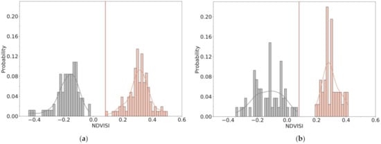
Figure 7.
The frequency histograms of minNDVISI values distribution of bare soil (grey colour) and grassland (red colour) classes: (a) sample points; (b) control points.
The left histogram (Figure 7a) shows the distributions of NDVISI index values frequency and profile curves of the bare soil and grassland sample points. There are clearly separated two classes’ peaks without any overlapping of two distributions. The optimal threshold between the two distributions was based on maximizing Cohen’s Kappa value and adjusted by visual check of five-year mosaic for the period 2006–2010. The resulting threshold value for the NDVISI index is 0.082 with Cohen’s kappa is 1.0, an observed probability is 1.0 and an expected probability is 0.506. Confusion matrix of “bare soil-grasslands” sample points is presented in Table 6.
Table 6.
Confusion matrix of “bare soil-grasslands” sample points classification with maximum Cohen’s kappa.
A threshold validation was carried out for the five-year minNDVISI image of 2020. We selected 54 bare soil points on Landsat mosaic image (2020) and 41 forest points from the field database. The right histogram (Figure 7b) shows the distributions of NDIVISI index values frequency and profile curves of the bare soil and grassland control points. The classes are located far enough on the histogram and do not overlap with each other. The accuracy of the recognition of the control points is the following: Cohen’s Kappa is 1.0, an observed probability 1.0 and an expected probability is 0.509. The confusion matrix is presented in Table 7.
Table 7.
Confusion matrix of “bare soil-grasslands” control points classification.
Additionally, we calculated the threshold for the PVI index [28] derived from Landsat mosaic image of 2010 to compare it with the threshold of our index. The soil line was calculated using the same points that were used to calculate the thresholds for our index. Figure 8a below shows histograms of the distribution of the PVI index of bare soil and grassland sample points.
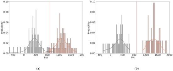
Figure 8.
The frequency histograms of PVI values distribution of bare soil and grassland classes: (a) sample points; (b) control points.
As well as our index, the PVI index has two distinct peaks and a high separability of two classes. As a result, the threshold value for the PVI index was 886, with Cohen’s Kappa 0.935, an observed probability was 0.968 and an expected probability was 0.506. The right histogram (Figure 8b) shows the distributions of PVI index values frequency and profile curves of the bare soil and grassland control points. The density of distributions is higher than for sample points of our index. The classes are also located far enough on the histogram and do not overlap with each other. The accuracy of recognition of control points is similar with our NDVISI index: Cohen’s kappa is 1.0, an observed probability is 1.0 and an expected probability is 0.509.
Thus, the validation has showed we can apply the thresholds fitted according to Landsat 2010 data to the indices of other time periods. The efficiency of both indices was equal for the 2015–2020 period, but NDIVISI had better discrimination ability for the 2006–2010 sample.
3.4. Forest Cover Dynamic Map and Its Analysis
Figure 9 shows the spatial distribution of forest cover during 1985–2020 time period for two bordering administrative districts with five-year intervals. We can see some pronounced changes of forest cover after 2000 in the district of Russia and Belarus.
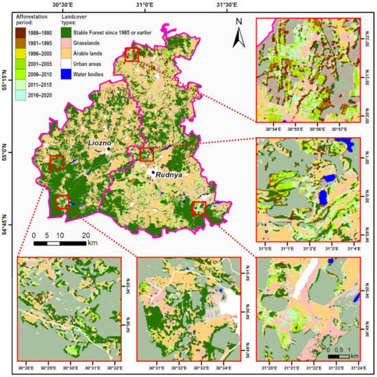
Figure 9.
Afforestation dynamics over the study area. Territories outside the IAL are lightened with semi-transparent overlay on the insert maps.
Such timing for the abundant changes is also clearly reflected by dynamics of total areas of forests, arable land and other categories within the bordering of the initial agricultural lands and administrative districts (Figure 10 and Figure 11).
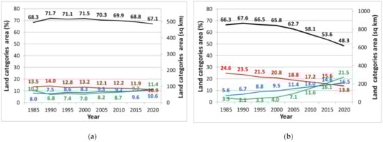
Figure 10.
The land categories dynamic within the IAL mask: (a) Liozno district (Belarus); (b) Rudnya district (Russia). Legend: arable lands (black), grasslands (red), afforested arable lands (green), afforested grasslands (blue).
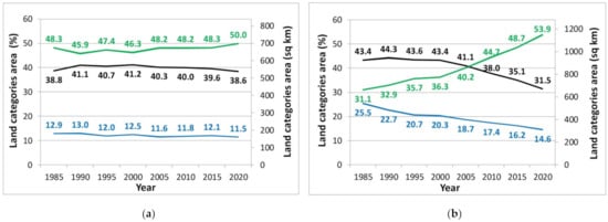
Figure 11.
The dynamic of the afforestation within the administrative districts: (a) Liozno district (Belarus); (b) Rudnya district (Russia). Legend: Arable lands (black), forest (green), other lands (blue).
Generally speaking, the reduction in the area of initial agricultural lands for the district in Russia is impressive. About 32% of the arable lands and grasslands in the Rudnya district (Russia) were afforested by the end of the considered period (1985–2020), while the same categories in the Liozno district (Belarus) decreased only by around 5%. The especially high rate of changes in forest cover of the Russian district of our study area has been observed after 2000. Before, the arable lands and grasslands were converted in forests only slightly and amounted to 4.8% over the first 15 years of the considered period.
Considering arable lands and grasslands separately, we have identified the following changes. Rudnya district has lost about 18 percent points (p.p.) of arable lands (from 66.3% in 1985 to 48.3%. in 2020) and 10.8 p.p. of grasslands (from 24.6% in 1985 to 13.8% in 2020). The rate of changes in arable lands intensified after the year 2000, while grasslands exhibited a relatively constant rate throughout the whole period. In the Republic of Belarus, arable lands shifted to forests during the monitoring period only by about 1.2 p.p. The afforestation of grasslands has increased by 2.6 p.p. relatively to 1985. The areas of forest on arable lands, forest on grasslands, arable lands and grasslands in sq. km for all five-year periods are given in Table S3 of the Supplementary Materials.
The dynamics of the area (in percent) of the forests, arable and other lands within the bordering administrative districts is shown in Figure 11. The forest area includes not only forests on agricultural lands, but forests growing on the forest lands of Russia and the Republic of Belarus. The arable lands are obtained using the integrated mask derived from five-year Landsat mosaics for 35 years. The “Other lands” category represents the lands that were not included into forest or into arable land masks. These include grasslands, swamps, urbanized areas (from OSM) and water masks derived from Landsat data.
The average reduction in arable land areas of the Rudnya district amounted to 7.26 square kilometers (sq. km) per year (sq. km/yr.) over the entire monitoring period. Before the year 2000 (in the 90s of the 20th Century), the reduction in area was slow, approximately 0.08 sq. km/yr. However, since 2000, the rate of change from arable lands to other land cover classes area increased and on average was 12.64 sq. km/yr. The opposite picture is observed with forests. The forest cover of the Russian district increased on average by 13.88 sq. km per year over the entire monitoring period. After year 2000, the rate of positive change of forest area also increased and on average amounted to 18.77 sq. km/yr. At the same time, the reduction of arable lands in Belarus district was 0.09 sq km/yr. and the forest cover increase with 0.68 sq. km/yr. for the entire period. Though less dramatically, the rate of change after 2000 also increased for arable lands and forests in comparison with the 1990s and amounted to 1.85 and 2.56 sq. km per year, respectively. The areas of the forests, arable and other lands in sq. km for all five-year periods are provided in Table S4 of the Supplementary Materials.
Clearly, we observed completely different afforestation trends in two bordering administrative districts. Our results, as well as some reasons and drivers of observed trends of afforestation of arable lands, are discussed in the next section.
4. Discussion
4.1. Landsat Mosaics
Since the forest cover mapping method used in our study was based on classification of the spectral index by a constant threshold, the quality of the satellite imagery utilized for index calculation was critical for obtaining reliable results. Considering the uneven temporal distribution of Landsat cloudless observations over the study area within the 1981–2020 period, which disables the opportunity for a consistent annual time-series generation, using a five-year period for mosaics composing, was the most suitable and simple option to acquire entire spatially continuous and seamless multi-temporal images. Moreover, in contrast to negative changes in forest cover caused by felling, fires and windfalls, natural afforestation is a long-lasting process that does not provide an instant effect on the surface reflectance values of satellite image pixels. According to the Russian National Greenhouse Gas Inventory Report [62], the average period of reforestation at clearcuttings in the Smolensk region is four years. However, the Russian legal minimum requirements for a stand to be considered as a young forest are 0.7–1.5 m height with stem density of 1500–2200 trees per ha, depending on the tree species. At the same time, most studies that utilize Landsat data for forest cover assessment are guided by FAO’s definition of forest, which states 5 m tree height and 10% canopy closure as minimum requirements. In addition, we are not aware of any studies, which were explicitly focused on Landsat image’s potential for reliable discrimination of young forests with different heights and density from the surrounding non-tree vegetation. Considering this ambiguity, it is still reasonable to assume, that the delay for Landsat-based forest cover identification should be much longer than four years, as the tree stands have to reach certain height and canopy closure values (which are converted to a certain SR value of pixels on satellite image) to be discriminated from other vegetation types at 30 m spatial resolution. Additionally, our results indirectly confirm this assumption, as a massive increase in forest area in Rudnya district was detected only in 2000s, while a large-scale abandonment of agricultural lands is generally associated with the collapse of the USSR in early 90s. Thus, the five-year period for mosaic composing seems to be acceptable for the afforestation dynamics assessment, at least in our case. On the other hand, this composing period is inappropriate for arable lands area estimation based on the bare soil identification, as ploughing generally is not carried out annually and at the same time throughout the year for each particular field. In this case, the five-year median-based composing causes massive omissions of bare soil area in the resulting mosaics due to its spectral characteristics (relatively high reflectance values). At the same time, replacing the median with another statistical function for composing (e.g., maximum or sorting according to special spectral index values) causes the massive artifacts occurrence. So, the annual median-based mosaics were used in our study alongside the five-year ones as a trade-off between the mosaic quality and the amount of bare soil on the resulting image, but only for generation of arable land’s maximum expansion mask and not for direct assessment of its temporal dynamics.
4.2. Forest Cover Index
Apart from Becker’s original work, there was only one successive research on FCI that we were able to find at the time of writing this paper. L. I. Feliciano-Cruz and co-authors implemented the same workflow over the same territory as in the original study, but with a single Landsat 7 scene [63]. The overall accuracy of tree/non-tree classification, which was based on the visually determined FCI threshold, ranged from 83.7 percent to 95.5 percent with Cohen’s kappa of 67.5 percent and 90.6 percent, depending on the test sampling scheme type (random or purposive). It is worth noting that all test samples were classified based on a visual interpretation of the 2 m WorldView-2 imagery. Water bodies and dark non-forest vegetation (such as dense crops) were stated as the main source of misclassification.
Results of our field-data-based validation confirm the FCI capability for forest and non-forest vegetation discrimination on Landsat images and its robustness for time series analysis, provided a sufficient harmonization of the initial imagery. However, according to visual analysis of index values’ spatial distribution, which was carried out during our study, two significant drawbacks in terms of thematic classification of land cover types must be accounted for: (1) FCI may misclassify forest with water and other dark objects (e.g., tall building shadow or dense non-tree vegetation), similarly to previous findings in Feliciano-Cruz’s research; (2) FCI cannot discriminate between forest and forested mires (including those with sparse tree cover). While the first issue can be partly solved by using more specific spectral indices (e.g., MNDWI for better water objects discrimination in our study), the second one remains challenging to address without any supplementary relevant geospatial data. In addition, further research is required to analyze the FCI sensitivity to the tree height and canopy closure variability of forest stands. Nevertheless, if the aim of classification is not to identify the forest in general across the Landsat image, but rather to discriminate tree cover from other vegetation types (such as croplands and grasslands in our case) within an appropriate predefined area of interest (IAL in our study), using FCI shall be a proper option.
4.3. Bare Soil Index (NDVISI)
Our assumption that the proposed NDVISI can distinguish bare soil and, accordingly, arable land with a fitted threshold, was confirmed. The sum of the reflectance values of the three visible bands was close to the value of the near infrared band. Thus, we were able to confidently separate vegetation from bare soil. Certainly, apart from arable land, some dark and light non-vegetation objects on the earth’s surface are also located on the left side of the NDIVISI histogram (e.g., water, forest shadows, burnt forests, forest clear cuts, urbanized lands), so the index does not allow to distinguish between them. Therefore, it is required to use other indices [64] or their combinations [59] to consistently exclude these objects from our area of interest. In our case, we localized initial agricultural land in advance using historical topographic maps and OSM urban layers, and the corresponding index was used to recognize water bodies [32]. As a result, we were able to use a simple combination of visible and near infrared bands to turn them into a vegetation index. Many authors use specialized indices (PVI, SAVI, etc.) for mapping arable lands [24,25]. We checked and found that, in our case, the use of NDVISI is on par with PVI. Therefore, we use NDVISI, as it is easier to calculate in our studies.
In addition, the advantage of applying NDVISI is that it is based solely on spectral bands that are available in many current very-high resolution satellite systems, for example, Sentinel-2 (10 m), Spot-6 (6 m), RapidEye (5 m), PlanetScope (3 m) and others [65], enabling us to combine multispectral images of different spatial resolution to identify the bare soil. This increases the frequency of observations per year and opens the possibility to investigate the condition of small agricultural fields (e.g., with PlanetScope or RapidEye).
4.4. Accuracy of Forest Cover Assessment
We obtained reliable results in terms of Kappa statistics during the identification and validation of indices thresholds, but a full-scale accuracy assessment of generated thematic products cannot be performed without a spatially and temporally distributed independent test sample. Although we lack such data, we can still compare our results with other geospatial products for the same area, that were previously obtained in similar studies. For this purpose, we used the “Eastern Europe Forest cover dynamics 1985 to 2012” dataset [66] produced by The Global Land Analysis and Discovery (GLAD) group at the University of Maryland [8]. Similar to our work, it is based on the assessment of Landsat imagery, and, therefore, contains the most straightforwardly comparable information. Forest cover estimates derived from this dataset for the two focal bordering districts were very close to ours (Table 8) with the maximum difference of 2.9 p.p. It can be considered as an additional confirmation of reliability for the developed method.
Table 8.
Comparison of forest cover values (%) for different years, assessed in our study (FCI) and ones derived from the GLAD group dataset (GLAD).
Regarding the potential sources of uncertainty in our forest cover estimates, several significant points should be mentioned. The estimates for the first (1985) and last (2020) slices of analysed time series are likely to be less accurate than for the inner ones, since the corresponding thematic masks cannot be properly checked for consistency (see Section 2.3.8). In particular, the forest cover values within IAL in 1985 were unexpectedly higher than in 1990 for both bordering districts, which can be caused by uncorrected misclassifications at the temporal edges of FCI mask. Following this logic, the forest cover values for 2020 could also be overestimated. Nevertheless, the most obvious inflection point of the forest cover dynamics curve (for the Russian district) corresponds to the year 2000, so these possible errors shall have little effect on the general trends.
Another source of potential errors in forest cover estimations is associated with inaccuracies in the used water and urban objects masks. While precise mapping of water and built-up areas, based on Landsat imagery, is a rather equally complex task as the forest cover assessment, in our study the main function of these masks was to reduce the number of misclassifications emerging after FCI and NDVISI thresholding. So, to keep our focus on forest cover, we chose relatively simple and robust, but not perfect methods to obtain thematic products for these landcover classes. Undoubtedly, both of them have their own level of accuracy, but since we used constant masks for the entire time series, the produced errors should be systematic and not affect the forest cover trends. Additionally, water and urban objects masks cover a total of only 3.5% of our study area, so it is unlikely that they can be considered as a major error source in our case at all. However, for consequent studies, we recommend adopting this element of our approach with caution, especially for urban objects. While MNDWI is a widely used, robust water index, the OSM data are very heterogeneous across different regions in terms of accuracy and detalization due to the way they are collected.
4.5. Natural Afforestation Drivers
Our results on forest cover trends in bordering districts are generally in line with our prior expectation, given that the natural afforestation dynamics in our case are directly related to the agricultural land abandonment processes, which have been thoughtfully studied in Russia and in other Eastern European countries by many authors [8,11,67,68,69]. At the regional level, the main factors determining the trends in agricultural land are both the dynamics of the rural population and natural conditions. Particularly for Nonchernozem European Russia (Non-Black Earth Zone), the demographic factor is shown to be determinative, while natural conditions typically only enhance or weaken its effect [70,71]. Prishchepov et al. [67] showed that the highest abandonment rate (46%) was observed in Smolensk region among other bordering regions of Russia. At the same time, in Belarus border districts, the share of abandoned agricultural lands was just 13 percent [72], which is significantly lower, not only compared to Russia, but also compared to post-Soviet neighbouring countries that have joined the European Union, such as Latvia and Lithuania [72,73]. Low abandonment rates in the Republic of Belarus are probably associated with the continuing strict state regulation of the agricultural sector. In addition, the contribution of the agricultural sector to total gross domestic product in Belarus was higher than of its neighbours, both before the collapse of the USSR and in the 1990s.
Abandoned agricultural lands, especially low-productive ones in many countries of the world, are considered as objects for restoration of biodiversity, ecosystem functions and services [74,75]. It has already been shown that the abandoned agricultural lands of Russia could act as an unprecedented carbon sink [6,18,76]. The total carbon sink in the Russian post-agrarian ecosystem is estimated to be in the range of 64 to 186 Mt C per year [18,76]. The differences in these estimates are due to different time periods, incompatibility of methods and models used and, most importantly, inaccurate official statistics on abandoned agricultural land [6].
The first legal regulation for forest-related processes on agricultural lands in Russia was established only in 2020. It governs planning and implementation of regimes for the use, protection and reproduction of forests located on agricultural lands in Russia [77]. Namely, it formally legalizes the existence and further self-development of forest ecosystems on all abandoned agricultural lands, which enables to officially account for and operate with these forest resources. Yet, sustainable management of such forests, assessment of their contribution to the absorption of greenhouse gases, maintenance of biodiversity, and the implementation of other ecosystem functions calls for further dedicated comprehensive studies.
5. Conclusions
In our study we developed a simple and robust method for forest cover dynamics assessment based on time series of Landsat imagery and limited field data. We applied it to test the method’s reliability and to reconstruct the natural afforestation dynamics over abandoned agricultural lands in the two bordering districts of Russia and Belarus, since it is a remarkable illustration of differences in the land management policy of the two countries. Obtained results are in good agreement with previous studies dedicated to agricultural lands abandonment and forest cover dynamics in the Eastern Europe region, which reflect known differences in the socio-economic and ecological aspects of the two analysed regions.
A relatively novel Forest Cover Index has been shown to be effective for forest cover discrimination, especially in the case of young forests on abandoned agricultural lands. However, it still has a number of limitations, at least within the described approach. Some further improvements are required to develop a general universally applicable method for forest mapping based on FCI. One option is to use a multi-seasonal imagery for index calculation, which may provide a better separability between tree and seasonal non-tree vegetation. Applying FCI to the Sentinel-2 imagery is also promising, as its MSI sensor contains three specific bands in the Red Edge spectral range, which provided better results than NIR when used for FCI calculation in Becker’s original study [33].
In our work, we demonstrated the possibility of using limited field data located close to the study area for the classification based on indices thresholding. However, this approach could limit the scalability of our method for larger areas, as optimal thresholds are likely to vary along the change of predominant young forest species that may have different SR properties. Therefore, it is crucial to enable an adaptive thresholding technique that would consistently combine the data on both local and global scales into a smooth spatial field. Nevertheless, such a development calls for further research with a series of cross-validation tests for different forest growing conditions and spatial levels (regional, continental, etc.).
Supplementary Materials
The following supporting information can be downloaded at: https://www.mdpi.com/article/10.3390/rs14020322/s1, Table S1: Geographic coordinates, observation year and land cover type of field plots, Table S2: Geographic coordinates and Landsat mosaic composing period for visually selected bare soil plots, Table S3: The dynamic of the afforestation within the IAL mask (sq. km), Table S4: The dynamic of the afforestation within the administrative districts (sq. km), Google Earth Engine script: Time series of Landsat mosaics generation with customizable composing period, R script: PIF-based mosaic normalization.
Author Contributions
Design of research and methodology, D.V.E. and E.A.G.; Landsat mosaics generation and normalization, E.A.G.; IAL mask and auxiliary GIS data, E.A.G., E.V.T. and N.V.K.; Landsat mosaic processing and validation, E.I.B. and E.A.G.; GIS analysis and statistic data, N.V.K.; field data collection, E.V.T. and A.V.T.; figures creation, E.A.G., E.I.B. and N.V.K.; writing—original draft preparation, D.V.E., E.A.G., E.V.T., E.I.B. and N.V.K.; writing—review and editing, D.V.E., E.A.G., E.V.T., O.V.S. and G.N.T.; Supplementary Materials preparation, E.A.G. All authors have read and agreed to the published version of the manuscript.
Funding
This research was supported by Russian scientific foundation: grant #21-74-20171 “Indicators of the agrogenic stage of forest development”. Cloud-free Landsat mosaics were generated in the framework of state funding contract “Methodological approaches to estimate structural organization and functioning of forest ecosystems” (# AAAA-A18-118052590019-7).
Institutional Review Board Statement
Not applicable.
Informed Consent Statement
Not applicable.
Data Availability Statement
The data presented in this study and not included in the Supplementary Materials are freely available as Google Earth Engine asset: https://code.earthengine.google.com/?asset=projects/ee-cepl/assets/smp_afforestation_masks (accessed on 10.01.2022), or on request from the corresponding author.
Acknowledgments
The authors are grateful to the staff of the Center for Forest Ecology and Productivity, in particular, Tatiana Braslavskaya for participation in field data collection. We also thank Vladimir Khokhryakov and Igor Bavshin from the Smolenskoe Poozerie National Park for their help in field work. We also acknowledge the Centre of collective usage «Geoportal», Lomonosov Moscow State University (MSU), for the provision of very high resolution satellite data over Smolenskoe Poozerie National Park territory.
Conflicts of Interest
The authors declare no conflict of interest.
References
- Ioffe, G.; Nefedova, T.; Kirsten, D.B. Land Abandonment in Russia. Eurasian Geogr. Econ. 2012, 53, 527–549. [Google Scholar] [CrossRef]
- Li, S.; Li, X. Global understanding of farmland abandonment: A review and prospects. J. Geogr. Sci. 2017, 27, 1123–1150. [Google Scholar] [CrossRef]
- Ustaoglu, E.; Collier, M.J. Farmland abandonment in Europe: An overview of drivers, consequences, and assessment of the sustainability implications. Environ. Rev. 2018, 26, 396–416. [Google Scholar] [CrossRef]
- Prishchepov, A.V. Agricultural Land Abandonment; Oxford Bibliographies. Environmental Science; Oxford University Press: Oxford, UK, 2020. [Google Scholar] [CrossRef]
- Prishchepov, A.V.; Muller, D.; Dubinin, M.; Baumann, M.; Radeloff, V.C. Determinants of agricultural land abandonment in post-Soviet European Russia. Land Use Policy 2013, 30, 873–884. [Google Scholar] [CrossRef] [Green Version]
- Schierhorn, F.; Muller, D.; Beringer, T.; Prishchepov, A.V.; Kuemmerle, T.; Balmann, A. Post-Soviet cropland abandonment and carbon sequestration in European Russia, Ukraine, and Belarus. Glob. Biogeochem. Cycles 2013, 27, 1175–1185. [Google Scholar] [CrossRef]
- Goga, T.; Feranec, J.; Bucha, T.; Rusnák, M.; Sačkov, I.; Barka, I.; Kopecká, M.; Papco, J.; Ot’ahel’, J.; Szatmári, D.; et al. A Review of the Application of Remote Sensing Data for Abandoned Agricultural Land Identification with Focus on Central and Eastern Europe. Remote Sens. 2019, 11, 2759. [Google Scholar] [CrossRef] [Green Version]
- Potapov, P.V.; Turubanova, S.A.; Tyukavina, A.; Krylov, A.M.; McCarty, J.L.; Radeloff, V.C.; Hansen, M.C. Eastern Europe’s forest cover dynamics from 1985 to 2012 quantified from the full Landsat archive. Remote Sens. Environ. 2015, 159, 28–43. [Google Scholar] [CrossRef]
- Estel, S.; Kuemmerle, T.; Alcantara, C.; Levers, C.; Prishchepov, A.; Hostert, P. Mapping farmland abandonment and recultivation across Europe using MODIS NDVI time series. Remote Sens. Environ. 2015, 163, 312–325. [Google Scholar] [CrossRef]
- Lesiv, M.; Schepaschenko, D.; Moltchanova, E.; Bun, R.; Dürauer, M.; Prishchepov, A.V.; Schierhorn, F.; Estel, S.; Kuemmerle, T.; Alcántara, C.; et al. Spatial distribution of arable and abandoned land across former Soviet Union countries. Sci. Data 2018, 5, 180056. [Google Scholar] [CrossRef]
- Global Mapping Hub by Greenpeace. Abandoned Agricultural Lands. 2019. Available online: https://maps.greenpeace.org/project/abandoned-agricultural-lands/ (accessed on 25 August 2021).
- Sieber, A.; Kuemmerle, T.; Prishchepov, A.V.; Wendland, K.J.; Baumann, M.; Radeloff, V.C.; Baskin, L.M.; Hostert, P. Landsat-based mapping of post-Soviet land-use change to assess the effectiveness of the Oksky and Mordovsky protected areas in European Russia. Remote Sens. Environ. 2013, 133, 38–51. [Google Scholar] [CrossRef]
- Koroleva, N.V.; Tikhonova, E.V.; Ershov, D.V.; Saltykov, A.N.; Gavrilyuk, E.A.; Pugachevski, A.V. Twenty-Five Years of Reforestation on Nonforest Lands in Smolenskoe Poozerye National Park According to Landsat Assessment. Contemp. Probl. Ecol. 2018, 11, 719–728. [Google Scholar] [CrossRef]
- Adoption of the Paris Agreement. 2015. Available online: http://unfccc.int/resource/docs/2015/cop21/eng/l09r01.pdf (accessed on 25 August 2021).
- Order of the Government of the Russian Federation. #670-r of 14 April 2015. Available online: http://publication.pravo.gov.ru/Document/View/0001201604200001 (accessed on 25 August 2021).
- Draft Concept on the Russian System of Circulation of Carbon Units. Ministry of Economic Development of the Russian Federation. 2020. Available online: https://www.economy.gov.ru/material/file/c9bc041a79280702939e7c28c4862f15/proekt_koncepcii.pdf (accessed on 25 August 2021).
- Queiroz, C.; Beilin, R.; Folke, C.; Lindborg, R. Farmland abandonment: Threat or opportunity for biodiversity conservation? A global review. Front. Ecol. Environ. 2014, 12, 288–296. [Google Scholar] [CrossRef]
- Kurganova, I.; Lopes de Gerenyu, V.; Kuzyakov, Y. Large-scale carbon sequestration in post-agrogenic ecosystems in Russia and Kazakhstan. Catena 2015, 133, 461–466. [Google Scholar] [CrossRef]
- Lukina, N.V.; Geraskina, A.P.; Gornov, A.V.; Shevchenko, N.E.; Kuprin, A.V.; Chernov, T.I.; Chumachenko, S.I.; Shanin, V.N.; Kuznetsova, A.I.; Tebenkova, D.N.; et al. Biodiversity and Climate-regulating Functions of Forests: Current Issues and Research Prospects. For. Sci. Issues 2021, 4, 1–90. [Google Scholar] [CrossRef]
- Food and Agriculture Organization of the Unites Nations. Global Forest Resources Assessment. 2020. Available online: https://www.fao.org/3/I8661EN/i8661en.pdf (accessed on 26 November 2021).
- Ma, L.; Li, M.; Ma, X.; Cheng, L.; Du, P.; Liu, Y. A review of supervised object-based land-cover image classification. ISPRS J. Photogramm. Remote Sens. 2017, 130, 277–293. [Google Scholar] [CrossRef]
- Potapov, P.; Hansen, M.C.; Kommareddy, I.; Kommareddy, A.; Turubanova, S.; Pickens, A.; Adusei, B.; Tyukavina, A.; Ying, Q. Landsat Analysis Ready Data for Global Land Cover and Land Cover Change Mapping. Remote Sens. 2020, 12, 426. [Google Scholar] [CrossRef] [Green Version]
- Liu, Y.; Liu, R. A Simple Approach for Mapping Forest Cover from Time Series of Satellite Data. Remote Sens. 2020, 12, 2918. [Google Scholar] [CrossRef]
- Bartalev, S.A.; Egorov, V.A.; Loupian, E.A.; Plotnikov, D.E.; Uvarov, I.A. Recognition of Arable Lands Using Multi-Annual Satellite Data from Spectroradiometer Modis and Locally Adaptive Supervised Classification. Comput. Opt. 2011, 35, 103–116. [Google Scholar]
- Kibret, K.S.; Marohn, C.; Cadisch, G. Use of MODIS EVI to map crop phenology, identify cropping systems, detect land use change and drought risk in Ethiopia–an application of Google Earth Engine. Eur. J. Remote Sens. 2020, 53, 176–191. [Google Scholar] [CrossRef]
- Plotnikov, D.E.; Kolbudaev, P.A.; Bartalev, S.A.; Loupian, E.A. Automated annual cropland mapping from reconstructed time series of Landsat data. Curr. Probl. Remote Sens. Earth Space 2017, 12, 112–127. [Google Scholar] [CrossRef]
- Yu, X.; Her, Y.; Zhu, X.; Lu, C.; Li, X. Multi-Temporal Arable Land Monitoring in Arid Region of Northwest China Using a New Extraction Index. Sustainability 2021, 13, 5274. [Google Scholar] [CrossRef]
- Tucker, C.J. Red and photographic infrared linear combinations for monitoring vegetation. Remote Sens. Environ. 1979, 8, 127–150. [Google Scholar] [CrossRef] [Green Version]
- Lehmann, E.A.; Wallace, J.F.; Caccetta, P.A.; Furby, S.L.; Zdunic, K. Forest Cover Trends from Time Series Landsat Data for the Australian Continent. Int. J. Appl. Earth Obs. Geoinf. 2013, 21, 453–462. [Google Scholar] [CrossRef]
- Ye, W.; Li, X.; Chen, X.; Zhang, G. A spectral index for highlighting forest cover from remotely sensed imagery. In Proceedings of the SPIE Asia-Pacific Remote Sensing, Land Surface Remote Sensing II, Beijing, China, 8 November 2014; p. 92601. [Google Scholar] [CrossRef]
- Acharya, T.D.; Subedi, A.; Lee, D.H. Evaluation of Water Indices for Surface Water Extraction in a Landsat 8 Scene of Nepal. Sensors 2018, 18, 2580. [Google Scholar] [CrossRef] [Green Version]
- Xu, H. Modification of normalized difference water index (NDWI) to enhance open water features in remotely sensed imagery. Int. J. Remote Sens. 2006, 27, 3025–3033. [Google Scholar] [CrossRef]
- Becker, S.J.; Daughtry, C.S.T.; Russ, A.L. Robust forest cover indices for multispectral images. Photogramm. Eng. Remote Sens. 2018, 84, 505–512. [Google Scholar] [CrossRef]
- Gribova, S.A.; Isachenko, T.I.; Lavrenko, E.M. (Eds.) Vegetation of the European Part of the USSR; Nauka: Moscow, Russia, 1980; 236p. (In Russian) [Google Scholar]
- Shkalikov, V.A. (Ed.) Nature of the Smolensk Region; Universum: Smolensk, Russia, 2001; 424p. (In Russian) [Google Scholar]
- Weather Archive in Liozno (Vitebsk Region). Available online: https://global-weather.ru/archive/liozno (accessed on 25 August 2021).
- Weather Archive in Rudna (Smolensk Region). Available online: https://global-weather.ru/archive/rudnya_rudnyanskij_rajon_smolenskaya_oblast (accessed on 25 August 2021).
- Municipal Formation of Rudnyansky District of the Smolensk Region. About Rudnyansky District. Available online: https://рудня.рф/leftmenu/events/ (accessed on 25 August 2021).
- Forestry Regulations of the Rudnyansky Forestry Department of the OGKU “SMOLUPRLES” Branch. Available online: https://les.admin-smolensk.ru/files/198/lhr-rudnyanskoe.pdf (accessed on 25 August 2021).
- State Forestry Institution “Lioznensky Forestry”. Available online: https://mlh.by/our-additional-activities/forestry-association/lioznenskiy-leskhoz/ (accessed on 25 August 2021).
- Lioznensky District Executive Committee. Agricultural Organizations. Available online: http://liozno.vitebsk-region.gov.by/ru/sel-org/ (accessed on 25 August 2021).
- Forest Management Regulations of “Smolenskoe Poozerie” National Park; Filial FGUP “Roslesinforg” “Zaplesproekt”: Moscow, Russia, 2015; 190p. (In Russian)
- Estimation of the Resident Population of the Smolensk Region as of 1 January 2021. Available online: https://sml.gks.ru/storage/mediabank/3lwbyaOX/MO21.pdf (accessed on 26 November 2021).
- The Population of the Liozno District by Sex and Individual Ages as of 1 January 2021. Available online: https://vitebsk.belstat.gov.by/upload/iblock/c4a/c4ae2e1abb06c616a1aa0c3822b3b9f1.pdf (accessed on 26 November 2021).
- Chronicle of Nature. 2014. Available online: http://www.poozerie.ru/files/442/%D0%9B%D0%B5%D1%82%D0%BE%D0%BF%D0%B8%D1%81%D1%8C%20%D0%BF%D1%80%D0%B8%D1%80%D0%BE%D0%B4%D1%8B%202014.pdf (accessed on 25 August 2021).
- Masek, J.G.; Vermote, E.F.; Saleous, N.E.; Wolfe, R.; Hall, F.G.; Huemmrich, K.F.; Gao, F.; Kutler, J.; Lim, T.K. A Landsat surface reflectance dataset for North America, 1990–2000. IEEE Geosci. Remote Sens. Lett. 2006, 3, 68–72. [Google Scholar] [CrossRef]
- Wulder, M.A.; Loveland, T.R.; Roy, D.P.; Crawford, C.J.; Masek, J.G.; Woodcock, C.E.; Allen, R.G.; Anderson, M.C.; Belward, A.S.; Cohen, W.B.; et al. Current status of Landsat program, science, and applications. Remote Sens. Environ. 2019, 225, 127–147. [Google Scholar] [CrossRef]
- The Worldwide Reference System|Landsat Science. Available online: https://landsat.gsfc.nasa.gov/about/worldwide-reference-system (accessed on 28 September 2021).
- Landsat 7. Available online: https://www.usgs.gov/core-science-systems/nli/landsat/landsat-7?qt-science_support_page_related_con=0#qt-science_support_page_related_con (accessed on 28 September 2021).
- Gorelick, N.; Hancher, M.; Dixon, M.; Ilyushchenko, S.; Thau, D.; Moore, R. Google Earth Engine: Planetary-scale geospatial analysis for everyone. Remote Sens. Environ. 2017, 202, 18–27. [Google Scholar] [CrossRef]
- OpenStreetMap. Available online: https://www.openstreetmap.org (accessed on 28 September 2021).
- Geofabrik Download Server. Available online: http://download.geofabrik.de/europe.html (accessed on 28 September 2021).
- Stuhler, S.C.; Leiterer, R.; Joerg, P.C.; Wulf, H.; Schaepman, M.E. Generating a Cloud-Free, Homogeneous Landsat-8 Mosaic of Switzerland Using Google Earth Engine. 2016. Available online: https://doi.org/10.13140/rg.2.1.2432.0880 (accessed on 28 September 2021). [CrossRef]
- Schott, J.R.; Salvaggio, C.; Volchok, W.J. Radiometric scene normalization using pseudoinvariant features. Remote Sens. Environ. 1988, 26, 1–14. [Google Scholar] [CrossRef]
- R Core Team. R: A Language and Environment for Statistical Computing. R Version 4.0.5. 2021. Available online: https://www.R-project.org// (accessed on 28 September 2021).
- Hijmans, R.J. Raster: Geographic Data Analysis and Modeling. R Package Version 3.4-13. 2021. Available online: https://CRAN.R-project.org/package=raster (accessed on 28 September 2021).
- Leutner, B.; Horning, N.; Schwalb-Willmann, J. RStoolbox: Tools for Remote Sensing Data Analysis. R Package Version 0.2.6. 2019. Available online: https://CRAN.R-project.org/package=RStoolbox (accessed on 28 September 2021).
- Wood, S.N. Generalized Additive Models: An Introduction with R, 2nd ed.; Chapman and Hall/CRC: Boca Raton, FL, USA, 2017; 496p. [Google Scholar] [CrossRef]
- Blasch, G. Multitemporal Soil Pattern Analysis for Organic Matter Estimation at Croplands Using Multispectral Satellite Data. Ph.D. Thesis, Technical University of Berlin, Berlin, Germany, 2017. Available online: https://www.researchgate.net/publication/320618072_Multitemporal_soil_pattern_analysis_for_organic_matter_estimation_at_croplands_using_multispectral_satellite_data (accessed on 26 November 2021).
- Cohen, J. A coefficient of agreement for nominal scales. Educ. Psychol. Meas. 1960, 20, 37–46. [Google Scholar] [CrossRef]
- Google Earth Web. 2021. Available online: https://earth.google.com/web/ (accessed on 30 August 2021).
- Russian Federation. 2020 National Inventory Report (NIR)|UNFCCC. Available online: https://unfccc.int/documents/226417 (accessed on 28 September 2021). (In Russian).
- Feliciano-Cruz, L.I.; Becker, S.J.; Lasko, K.D.; Daughtry, C.S.; Russ, A.L. Forest Cover Index for Tree Cover Detection Using Landsat-7 Multispectral Imagery. 2019. Available online: https://scholar.googleusercontent.com/scholar?q=cache:tWhmR8OBTGoJ:scholar.google.com/&hl=ru&as_sdt=2005&sciodt=0,5 (accessed on 28 September 2021).
- Huang, C.; Song, K.; Kim, S.; Townshend, J.R.G.; Davis, P.; Masek, J.G.; Goward, S.N. Use of a dark object concept and support vector machines to automate forest cover change analysis. Remote Sens. Environ. 2008, 112, 970–985. [Google Scholar] [CrossRef]
- A Database for Remote Sensing Indices. Available online: https://www.indexdatabase.de/db/bs.php?sensor_id=0 (accessed on 28 September 2021).
- Eastern Europe Forest Cover Dynamics 1985 to 2012|GLAD. Available online: https://glad.umd.edu/dataset/eastern-europe-forset-cover-dynamics-1985-2012 (accessed on 24 December 2021).
- Prishchepov, A.V.; Radeloff, V.C.; Baumann, M.; Kuemmerle, T.; Müller, D. Effects of Institutional Changes on Land Use: Agricultural Land Abandonment during the Transition from State-Command to Market-Driven Economies in Post-Soviet Eastern Europe. Environ. Res. Lett. 2012, 7, 024021. [Google Scholar] [CrossRef]
- Maslov, A.; Gulbe, A.; Gulbe, Y.; Medvedeva, M.; Sirin, A. Assessment of the situation with the overgrowth of agricultural lands with forest vegetation on the example of the Uglich district of the Yaroslavl region. Sustain. For. Manag. 2016, 4, 6–14. [Google Scholar]
- Lezhnin, S.A. The use of satellite data in the assessment of reforestation on the abandoned agricultural lands in Yaransk district of the Kirov region. For. Ecosyst. Clim. Chang. Biol. Product. Remote Monit. 2020, 6, 160–171. [Google Scholar] [CrossRef]
- Lyuri, D.I.; Goryachkin, S.V.; Karavaeva, N.A.; Denisenko, E.A.; Nefedova, T.G. Dynamics of Agricultural Lands of Russia in XX Century and Postagrogenic Restoration of Vegetation and Soils; Geos: Moscow, Russia, 2010; 415p. (In Russian) [Google Scholar]
- Kolosov, V.; Medvedev, A.; Zotova, M. Comparing the development of border regions with the use of GIS (the case of Russia). Geogr. Pol. 2017, 90, 47–61. [Google Scholar] [CrossRef] [Green Version]
- Prishchepov, A.V.; Müller, D.; Baumann, M.; Kuemmerle, T.; Alcantara, C.; Radeloff, V.C. Underlying Drivers and Spatial Determinants of post-Soviet Agricultural Land Abandonment in Temperate Eastern Europe. In Land-Cover and Land-Use Changes in Eastern Europe after the Collapse of the Soviet Union in 1991; Gutman, G., Radeloff, V., Eds.; Springer International Publishing: Cham, Switzerland, 2017; pp. 91–117. [Google Scholar] [CrossRef]
- Rendenieks, Z.; Nita, M.D.; Nikodemus, O.; Radeloff, V.C. Half a century of forest cover change along the Latvian-Russian border captured by object-based image analysis of Corona and Landsat TM/OLI data. Remote Sens. Environ. 2020, 249, 112010. [Google Scholar] [CrossRef]
- Navarro, L.M.; Pereira, H.M. Rewilding abandoned landscapes in Europe. Ecosystems 2012, 15, 900–912. [Google Scholar] [CrossRef] [Green Version]
- Benayas, J.M.R.; Bullock, J.M. Restoration of biodiversity and ecosystem services on agricultural land. Ecosystems 2012, 15, 883–889. [Google Scholar] [CrossRef]
- Kurganova, I.; Lopes de Gerenyu, V.; Six, J.; Kuzyakov, Y. Сarbon cost of collective farming collapse in Russia. Glob. Chang. Biol. 2014, 20, 938–947. [Google Scholar] [CrossRef]
- Resolution of the Government of the Russian Federation of 18 September 2020 #1482. Available online: http://government.ru/docs/all/129924/ (accessed on 21 October 2021).

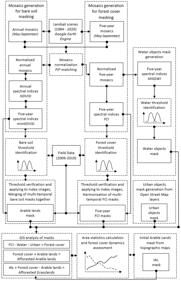
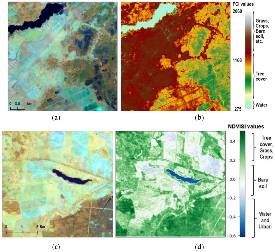


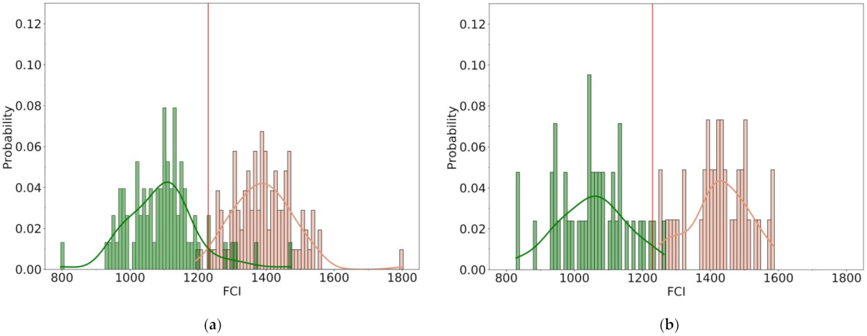
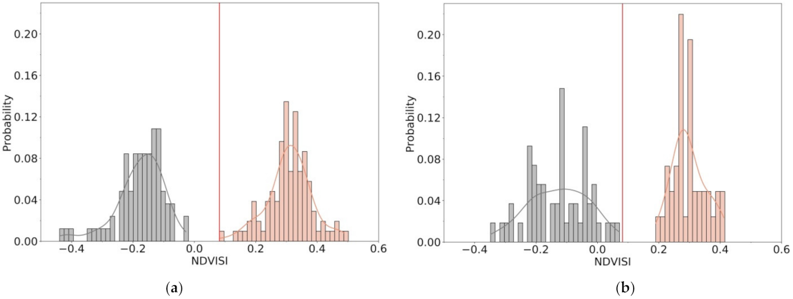
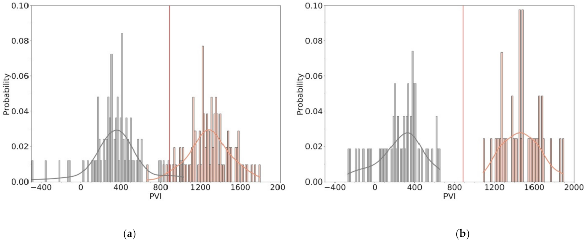
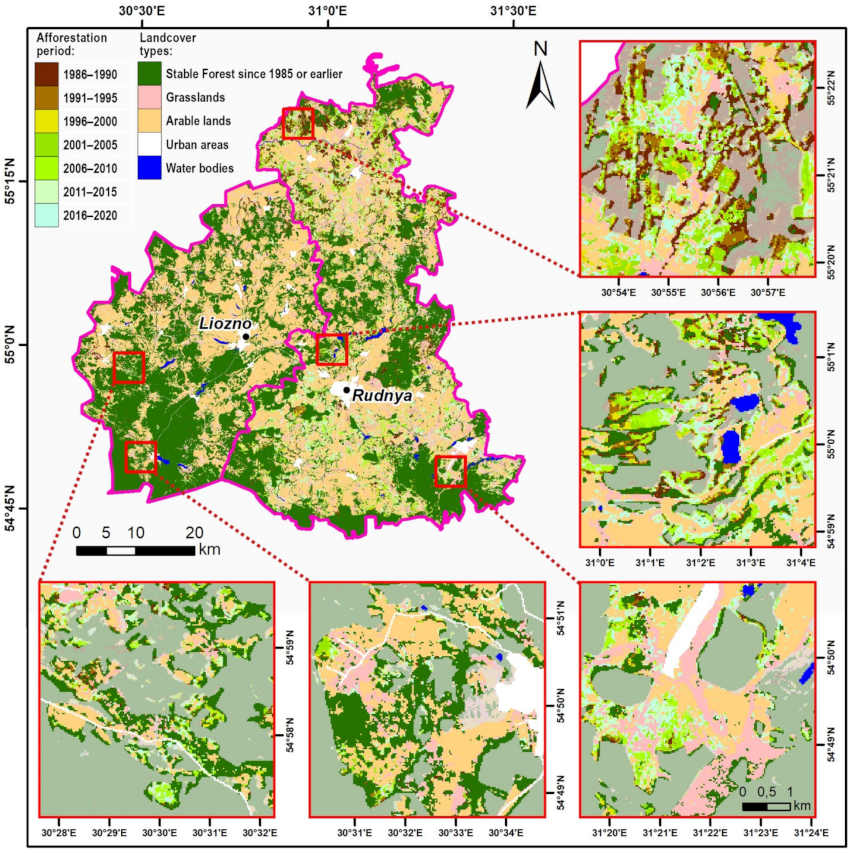
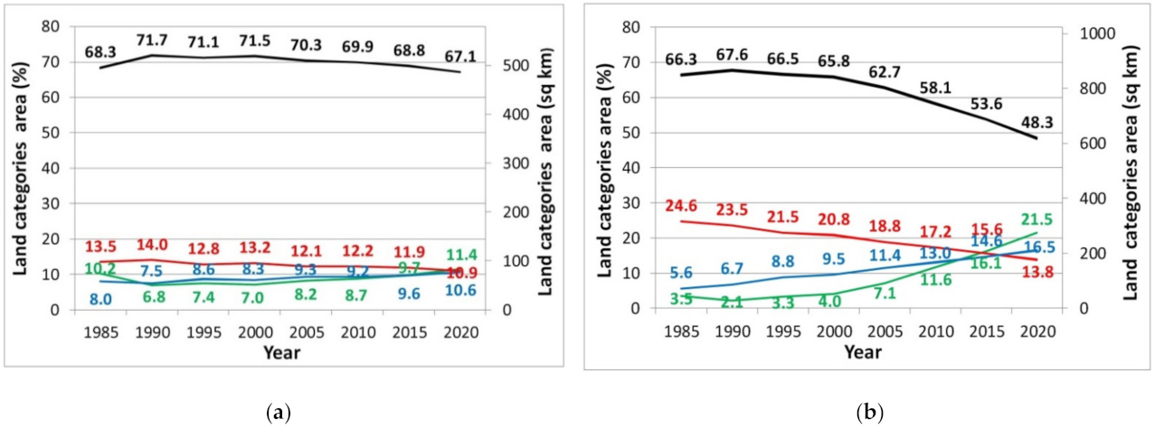
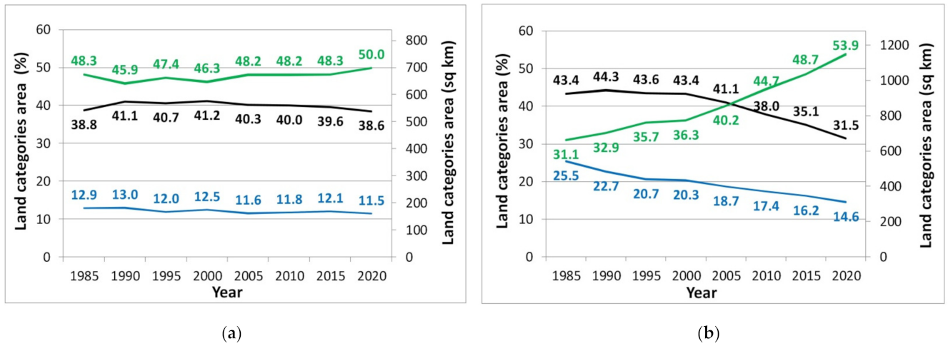
Publisher’s Note: MDPI stays neutral with regard to jurisdictional claims in published maps and institutional affiliations. |
© 2022 by the authors. Licensee MDPI, Basel, Switzerland. This article is an open access article distributed under the terms and conditions of the Creative Commons Attribution (CC BY) license (https://creativecommons.org/licenses/by/4.0/).