Abstract
Data about users is collected constantly by phones, cameras, Internet websites, and others. The advent of so-called ‘Smart Things’ now enable ever-more sensitive data to be collected inside that most private of spaces: the home. The first step in helping users regain control of their information (inside their home) is to alert them to the presence of potentially unwanted electronics. In this paper, we present a system that could help homeowners (or home dwellers) find electronic devices in their living space. Specifically, we demonstrate the use of harmonic radars (sometimes called nonlinear junction detectors), which have also been used in applications ranging from explosives detection to insect tracking. We adapt this radar technology to detect consumer electronics in a home setting and show that we can indeed accurately detect the presence of even ‘simple’ electronic devices like a smart lightbulb. We evaluate the performance of our radar in both wired and over-the-air transmission scenarios.
1. Introduction
It is no surprise that “smart” consumer electronics (e.g., devices that have computational and communication capabilities) are becoming fully integrated into our daily lives. Many smart devices are becoming a common fixture in homes—and yet their presence may not be readily apparent. For example, in many homes today, we find easy-to-spot smart assistants such as Amazon Echo [1] or Google Home [2], but we also find smart devices that are more difficult to visually detect, such as smart light bulbs [3], smart door locks [4], or smart refrigerators [5]. Many of these devices have traditionally lacked computational and communications capabilities, and the smart versions may be easily mistaken for their traditional “dumb” counterparts. Other devices, such as surveillance cameras and microphones, may be purposefully located in difficult-to-observe locations to collect data without making their presence known. Furthermore, the list of commercially available smart home devices grows every day, and research suggests the number of devices in a home may grow exponentially over the coming years [6]. In the near future, a home could easily contain dozens or hundreds of smart devices. The ubiquity of these devices will make it difficult to discover all of the devices present in a smart home environment. In this paper, we present our initial experiments using a harmonic radar to discover all types of smart devices in a home—even those that are powered off. Our approach works irrespective of the device’s communication protocols (e.g., Wi-Fi, Bluetooth, Zigbee) and should even detect malicious devices attempting to evade detection.
1.1. Motivation
As a motivating example, consider a scenario in which Alice sells her smart home to Bob. Alice will likely take many smart devices with her when she leaves the home for the last time, but she may also leave many devices behind. For instance, Alice may leave a smart thermostat behind. Researchers have shown that a surprising amount of information about the behavior of a home’s occupants can be inferred from devices that were not originally intended to collector behavior information. For example, water flow sensors on a pipe can determine when the home is occupied and in some cases can identify which person is home [7]. Other devices such a robot vacuum cleaner can use its Lidar sensor to record conversations between people inside the home [8]. The presence of these seemingly innocuous devices can lead to serious security or privacy leaks.
As the new home owner, Bob will likely want to know what devices are present, what is their function, and who has control over access to them. The last point is particularly salient for devices with obvious security and privacy implications (such as smart door locks and surveillance cameras), but is also important for devices with less obvious security and privacy implications as discussed above. The process of taking ownership of the new home, however, starts with detecting the presence of devices in the home. In this paper, we focus on the discovery problem.
1.2. Harmonic Radar for Device Discovery
Our approach leverages prior work done on harmonic radar [9]. A harmonic radar transmits a signal at a known frequency and listens for a return signal on a harmonic of the transmitted frequency (e.g., i times the transmitted frequency, where i is an integer greater than or equal to 1). If the transmitted signal encounters a non-linear junction (common in electronic devices, see below), it reflects the transmission at harmonic frequencies. When the transmitted signal encounters obstacles without a non-linear junction, this reflection does not occur [10]. Our system leverages this reflection characteristic by transmitting on one or more frequencies while listening for reflections on the first harmonic of the transmit signal. A signal received at a harmonic frequency indicates the presence of a smart device.
Transistors are a basic component of modern electronic devices and are an example of a non-linear junction. Transistors are composed of semiconducting materials that are created by introducing impurities to the crystalline structure of different chemical elements (a process known as “doping”), particularly silicon. Using doping, transistors sandwich layers of n-type (negative type) silicon that have extra electrons, and p-type (positive type) silicon that have fewer electrons. This arrangement creates sharp, non-linear, junctions where different types of silicon meet. Diodes, amplifiers, mixers, and rectifiers are other examples of non-linear electronic components [11,12]. These types of components are found in virtually all smart devices. (As an order of magnitude reference, there are approximately 64 billion transistors in 8 GB of RAM.)
Man-made metal-to-metal junctions, such as the ones present in semiconductors or in oxidized metals, have the ability of transforming the received signal and generating a harmonic frequency. This is referred to in the literature as spectral regrowth [10]. One of the possible responses is taking the incident radio waves and reflecting back a series of waves at harmonics of the original frequency. We have built on this non-linear phenomenon and, following the literature in the area of harmonic radars, implemented a proof-of-concept system that can detect the presence of consumer electronics in a noisy environment.
Non-linear or ‘harmonic’ radars were first introduced in the 1970s; since then, the range of applications for this technology has grown [9]. Harmonic radars have been used in self-driving vehicles to detect obstacles [13], in military applications to find explosives, in ecology to track insects and study bee pollination [14,15,16], in remote-sensing to sense temperature changes [17,18], and most recently, in maritime search and rescue efforts to locate castaways [19]. We now propose to leverage this technology and principles to build a sensory system that can identify electronic devices in smart homes.
There are three main challenges in using harmonic radios for this application. First, radar systems typically require highly specialized hardware. Second, harmonic radars are sensitive to radio frequency interference (RFI) present in the environment [12]. Third, consumer electronics vary in terms of size, composition, function, radio capabilities, power source, and more. To address these concerns, we first limit ourselves to off-the-shelf parts for the construction of our system and as well as for the devices being tested (i.e., we do not design any of the components). Then, we incorporate robustness to noise into the design and testing of our system. Any solution proposed must be able to identify target devices regardless of the normal chatter coming from Wi-Fi routers, Bluetooth wearables, cellular telephones, cordless telephones, ambient radio and television broadcasts, and more. Finally, we test a wide range of devices; varying size, functionality, and manufacturer, among others; and multiple examples per device.
1.3. Harmonic Radar Use Cases
Recalling the story about Alice and Bob, we envision a new “device inspection” stage in a home sale, similar to a structural engineer’s examination of the home’s integrity. In the device inspection, a professional inspector might use our harmonic radar to sweep the home to inventory all electronic devices, even hidden devices. This inventory might include the device type and its location within the home. This inventory can allow the seller to ensure they have removed any personal information from the devices left behind and can allow the buyer to take control of (or change) any device credentials, such as passwords or cryptographic keys.
A consumer version of our harmonic-radar system might be used to sweep temporary quarters such as hotel rooms or Airbnb homes for hidden cameras or microphones. (The popular press recently documented instances where spying devices were left in such lodging [20].)
1.4. Contributions
In this paper, we make some important contributions:
- We propose harmonic radar as a means to identify the presence of electronic devices in a home environment.
- We present proof-of-concept results for wired and over-the-air experiments.
- We examine previously unexplored frequencies between 2–2.8 GHz for harmonic radar.
- We base our work, both the radar and the target devices, on commercial equipment instead of on custom made components. This constraint makes the technology more available for researchers.
2. Related Work
Our system attempts to detect the presence of smart devices in a home, but one can envision other techniques. In this section, we briefly describe approaches from the literature. None accomplish our goal of detecting all devices in a home.
2.1. Sniffers
One common approach to detect devices is simply to set up a sniffer to listen for device transmissions and to record identifiers such as a MAC or IP address. This approach can certainly detect some devices, but has many serious shortcomings if the goal is to detect all smart devices. For example, a sniffer typically only observes one protocol. A Wi-Fi sniffer, for instance, can detect and decode Wi-Fi traffic, but normally cannot detect Bluetooth or Zigbee communications. Additionally, some devices might use analog communications (such as cordless phones); these would not be detected by a digital sniffer, even if the sniffer were capable of monitoring and decoding all common digital communication protocols.
Furthermore, even if the sniffer can decode a communication protocol, it must observe the same frequency used by the transmitting devices. A Wi-Fi sniffer, for example, must operate on the same band as the transmitter (2.4 GHz or 5 GHz), and be listening on the transmitter’s channel. Wi-Fi’s 2.4 GHz band has 14 different channels and its 5 GHz band has 70 different channels. Each channel is centered on a different frequency. Most Wi-Fi sniffers are unable to cover all possible channels.
Finally, sniffers can detect some transmitting devices, but cannot detect devices that do not transmit (such as a camera or microphone that stores data on a removable media) or communicate on wired network connections (such as Ethernet or landline telephone). Additionally, by design, some malicious devices may use communication techniques deliberately designed to evade detection [21].
Our approach can find devices regardless of their communication protocol—even if they do not transmit or are powered off.
2.2. Device Discovery Protocols
Numerous device-detection protocols have been proposed and some have made their way into commercial products. Cabrera et al. provide a survey of many of these types of discovery protocols [22]. Discovery protocols, however, rely on cooperative devices. They expect that, given some query by a device, other devices will respond to the query with truthful information about their identity and capabilities. Two problems prevent this approach from meeting our goal of discovering all devices in a home. First, devices must be aware of the discovery protocol; legacy devices may not be aware of the new discovery protocols. Second, malicious devices may attempt to evade detection by ignoring discovery queries, or perhaps worse, may masquerade as legitimate devices.
Our harmonic radar approach does not suffer from these drawbacks. It can discover devices without their cooperation—even when they are powered off.
2.3. Harmonic Radar
Literature in the topic of harmonic radars can be grouped into one of three categories: the design of the radar and its components [19,23,24,25,26,27], the detection of nonlinear circuits and the mathematical modeling and analysis of this behavior [12,23,27,28,29,30,31], and applications in which this technology is useful [13,14,15,17,18,32].
Our work most closely resembles the second area: the detection of nonlinear targets. The relevant literature is focused on counter surveillance applications. In a sense this is exactly were our work fits in, we are detecting unwanted electronics in a space. Our main contribution is that we focus on consumer electronics and test them in frequencies they are likely to respond. Most published work detects individual semiconductors (i.e., a PCB targets, integrated circuits, RFID tag); in reality, these are components of more complex electronics. The most complex target published has been a walkie-talkie radio both with the signal being fed directly through the antenna port or wirelessly as a moving target [31,33]. One gap in the literature, which we begin to address, is demonstrating the effectiveness of nonlinear responses when the devices are shielded and when the signal is passing through multiple (i.e., millions) nonlinear junctions, as is the case in out-of-the-box electronics [9].
3. Harmonic Radar
Detection and ranging technologies, described in Figure 1, are systems that combine a transmitter that sends a signal over some medium (often water or air), a target that responds to the signal, and a receiver that captures the response. The signal being transmitted can be affected by the transmission channel, obstacles in the signal’s path, the target, and noise. Modeling and characterizing any of these systems typically involves finding the relationship between the outgoing and the incoming signal. Linear systems have two characteristics: they are homogeneous and they follow the principle of superposition. Homogeneity refers to the scalar relationship between input and output, i.e., the transmitted signal and the return signal change proportionally with each other. Superposition is the ability of the system to generate a response that can be decomposed into the sum of the individual elementary signals. Any system that is not homogeneous and for which superposition does not hold true is called a nonlinear system [10,11].
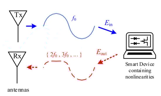
Figure 1.
Overview of the radar proposed for this work. The nonlinear circuits in the smart device modify the probe signal (in blue), emanating a return signal (in red) with additional harmonics.
Junction points between two metals have a nonlinear response to radio signals. Harmonic radars fall inside the umbrella term of ‘detection and ranging technologies’ and are designed to capture the response emitted by electronic targets. Previous work describes the mathematical relationship between the transmitted signal and the response (generated by the junctions found in electronics) as a memoryless power series [33,34,35]. We begin by describing the transmitted waveform as a sinusoid of the form
where is the electric field of the transmitted signal and is the amplitude of the electric field incident on the target (i.e., the received signal). The nonlinear response can be approximated by the power series
are the complex coefficients of the power series and is the electric field reflected from the target. In our system, we expect the nonlinear (harmonic) response to behave as follows:
where and is the frequency of the probe (i.e., transmitted) signal.
The first term is the linear response, as reflected or distorted by many objects radar’s path. Metals, fluids, and construction materials (i.e., clutter) will either reflect or attenuate the signal at this frequency. All subsequent terms (e.g., , ) represent the electronic nonlinearity. From Figure 1 we can see that the sinusoid with frequency (i.e., ) is the only signal transmitted in the system. When passes through a nonlinear target, it is reflected back at an integer multiple of the transmit frequency. Any signal present at the receiving antenna (Rx) listening on frequencies (in our case ) confirms the presence of the target in the path.
4. Experimental Setup
To build confidence in this method and demonstrate the ability of the harmonic radar to identify common electronic devices, we developed two experimental testbeds; one fully connected by wire and one over the air. The only difference between wired and the over-the-air experiments is the transmission channel: in the wired experiments, the transmitter was wired to a target object, allowing us to explore the potential for harmonic radar without regard for ambient RF effects; in the wireless experiments, all transmissions and reflections occurred through the air. In the remainder of this section, we describe the testbeds and the factors that could affect our measurements.
All experiments were conducted in an active residential apartment, complete with conventional furniture, electronics, occupants, and neighbors. Section 6 and Section 7 present measurements for 18 devices in both the wired and wireless configuration.
4.1. Hardware
In contrast to many harmonic radar applications, we built our system from off-the-shelf components; although we purchased hardware specialized for RF circuits, none were custom made. We identified six hardware modules necessary to run both the wired and wireless configurations, shown in Figure 2 and Figure 3.
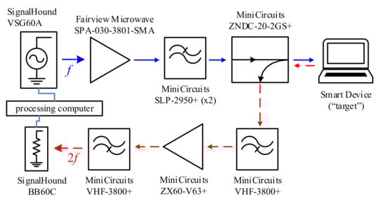
Figure 2.
Block description of the wired configuration of the radar system designed to detect home consumer electronics.
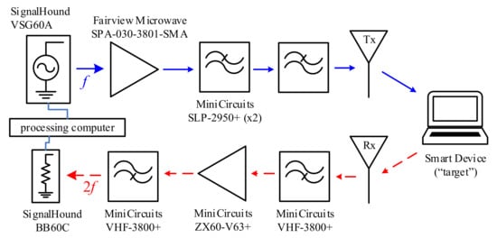
Figure 3.
Block description of the wireless configuration of the radar system designed to detect home consumer electronics.
We selected the SignalHound VSG60A [36], with a range between 50 MHz and 6 GHz, as the signal generator, and selected the SignalHound BB60C [37], with a range of 9 kHz to 6 GHz, as the spectrum analyzer. The wide range of both devices gives us the flexibility of testing a variety of frequencies while being able to capture the second harmonic. Both SignalHound products have USB connections that link each device to a processing computer equipped with a proprietary graphical interface and a programming API with a Python wrapper. We used an HP Spectre laptop running Windows 10 as the control and processing unit for the experiments. The APIs provided by the manufacturer allowed for automated experiments and reproducible results.
For the remaining four components, there are two types of filter and two amplifiers. In the outgoing circuit (indicated by the blue line in Figure 2 and Figure 3), we added two Mini Circuits SLP-2950+ low pass filters that allow the base frequency to go through while attenuating harmonics generated by the VSG60A. Similarly, in the return path (indicated by the red line in Figure 2 and Figure 3) we included two Mini Circuits VHF 3800+ that attenuate the base signal while allowing through any harmonic response. In terms of amplifiers, the outgoing circuit includes a Fairview Microwave SPA-030-3801-SMA power amplifier, which offers a 38 dBm gain over the input signal. The maximum power output by the VSG60A is 20 dBm (0.1 W). The power amplifier allows us to test and adjust the power level without saturating the signal generator. The role of both filters and amplifiers is to strengthen and clean the signals, reducing the noise generated by the components in the circuit.
In the wired setup (Figure 2), we used the MiniCircuit ZNDC-20-2GS+, a coupler with 10 dB attenuation on the return listening port. The three ports of the coupler served to connect transmitter, receiver, and test device; while allowing us to measure the transmitted signal after it had interacted with the test device.
In the wireless setup (Figure 3), we used two NI WA5VJB Log Periodic Antennas to transmit and receive the signals. The device being tested was placed equidistant to both antennas.
Finally, the last piece of hardware in the circuit is the target: the device being tested. In each experiment we used one of 16 distinct devices shown in Figure 4 and described in Section 6.1.
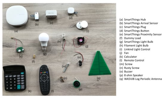
Figure 4.
An image of the target devices used in our experiments, along with the antenna (q) used for transmitting and receiving the probe signal. Not shown in the picture is the laptop shown later in Figure 10.
4.2. Frequency
Where most of the literature on harmonic radar focuses on UHF frequencies, there is a niche for devices that are around the Wi-Fi band [19]. The choice of frequency is often tied to the range of the radar. Lower frequencies have longer wavelengths and are able to travel much farther, and through more clutter, than higher frequencies. Intuitively, compare the range of FM radio stations (87.5–108 MHz) against the range of a Wi-Fi router (2.4 GHz). Radars are generally, though not exclusively, designed to look for targets kilometers ahead of the transceiver. For the purposes of our work a range of km is not necessary. We are interested in detecting devices within the boundaries of a room inside a home. Our range of interest is at most 100 m which allows us more flexibility in the choice of transmit frequency.
Furthermore, previous work shows that, because of RF noise regulations and shielding material built into their design, target devices are more likely to generate harmonics at frequencies they are intended to operate [38]. We are interested in finding devices that operate within the S-Band range (i.e., Wi-Fi, Zigbee, Bluetooth). We therefore expect that we’ll be most successful at detecting harmonics in a range of 4–8 GHz.
In summary, we transmit a sinusoid of constant frequency (i.e., 2.35 GHz, discussed in Section 6.2.1). In future works, we can explore the effect of different waveforms as a means to increase either the range or the performance of the radar.
4.3. Linearity
One key design decision for a harmonic radar system is transmitting a signal strong enough so that the lower power harmonics are detectable by the receiving antenna.
The signal generator will have two inherent limitations. First, the maximum power output of the signal generator is much lower than the level necessary to receive a detectable harmonic. In this work, the VSG60A has a maximum power output of 20 dBm, which is the equivalent of 100 mW; some literature indicates a need for power as high as 1 W for a continuous wave radar [9]. This constraint makes necessary the addition of the power amplifier to the transmission line. The second limitation is that the components required in the RF circuit for generating and measuring the signals are electronic devices in their own right. RF noise leaks will interact with devices and generate harmonics at the same range as the targets in the study.
The two main challenges stemming from the limitations are then: first, transmitting a strong harmonic-free signal from the outgoing channel; and second, extracting a low-power signal close to the noise floor of the spectrum analyzer [24]. The solution lies partially in the addition of low-pass filters to the transmit channel (i.e., attenuating any harmonics generated by the system) and high-pass filters to the receive channel (i.e., attenuating the linear response). While filters reduce (or eliminate) false positives by cleaning the signals, the solution is complete when the Low Noise Amplifier boosts the received signal to a level where the analog-to-digital converter in the spectrum analyzer will capture information contained at .
4.4. Distance and Signal Degradation
In free space, the harmonic power received from a nonlinear target is mathematically modeled by a modified version of the classical Friis transmission equation for a radar whose transmitter and receiver are co-located [11,19,28]. This nonlinear Radar Cross Section equation is given by
where TX identifies the transmitter and RX the receiver, P indicates power, G is the gain at the antennas, is the fundamental (or base) frequency wavelength, R is the distance to the target device, and is the radar cross-section of the target device. In this situation, may be considered a conversion loss between the transmitted probe frequency and the harmonic generated by the target device.
It should be noted that Equation (4) holds for a second-harmonic interaction, i.e., assuming that only the squared term from Equation (2) is retained. For higher-order interactions (i.e., higher harmonics, which would require tuning the receiver to higher frequencies), the terms on the right of Equation (4) including R would be raised to a higher integer power. Thus the falloff of the received signal for greater distances would be even more drastic.
Mathematically, responses from nonlinear targets are typically very weak because values for range from to m/W. Power incident on the target falls off with distance away from the transmitter, according to the one-way (linear) Friis equation, by a factor of . This incident power is then squared by the power-series law of Equation (2) giving and multiplied by the other terms in Equation (4) including . With the transmitter and receiver co-located, power captured by the receiver also falls off with distance away from the target by , which when multiplied by the gives the theoretical .
In a practical scenario, the received signal will be further reduced by effects such as multipath (multiple signal reverberations between the target and the receiver) and obscuring/shadowing of the target by walls, furniture, appliances, or other obstacles. Because the typical values for are so small, the power transmitted by a harmonic radar generally must be orders-of-magnitude higher than a traditional (linear) radar to achieve a comparable signal-to-noise ratio. This disadvantage, however, trades off against the chief advantage of harmonic radar, which is clutter rejection.
Electronics generate harmonics; nearly all other materials and devices do not. Some electronic devices (e.g., smart switches, buzzers, calculators) are so small that they appear to traditional radar as noise or (at best) weak clutter items. However, even at distances of meters are more, electronics smaller than a fingernail are still detectable using harmonic radar [23]. In other words, though the power required to achieve practical detection distances for harmonic radar is high (i.e., Watts or more), this type of radar has the ability to detect electronic targets that would otherwise be undetectable by traditional radar.
For our study, our targets are not obscured, our antennas are co-located, and there is a direct line-of-sight between the targets and the antennas. Thus, following Equation (4), we expect the harmonic responses received from our nonlinear targets to fall as as we increase the distance between our Tx/Rx antennas and the electronic devices.
4.5. Performance Metrics
In this work, we determine whether a device is linear or nonlinear based on the strength of the received second harmonic. For the wired experiments, a 5 dBm difference between the noise floor and the received signal strength would indicate the presence of a nonlinear target. For the wireless dataset, we considered the power loss from the over-the-air transmission by signal generator and decided that a 3 dB signal would identify the nonlinear component. The selection of the thresholds is discussed in greater detail in the results (Section 6).
5. Experimental Baseline
Figure 5 presents the spectrum trace around 4.7 GHz. On the left, Figure 5a, shows the signal strength at all frequencies when the signal generator is transmitting and there is no test device in the circuit. All we see in the trace is background noise around −136 dBm. On the right, Figure 5b, shows the trace around the same frequency window for when the proximity sensor is connected. In the signal generator, the frequency is set at 2.35 GHz at a power of 10 dBm. The response, recorded on the screenshot, captures at the second harmonic a signal strength of −122.8 dBm. The only change to the circuit and the settings is the addition of the sensor. Without analyzing the power or effect of the harmonics generated by each of the components, in recording both measurements (and the difference between them), we are reasonably certain that the source of the signal is the sensor.
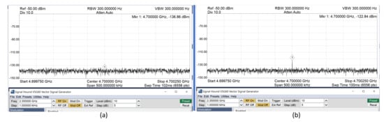
Figure 5.
Screenshot of the spectrum plot for the second harmonic. (a) shows the spectral plot when there are no devices present in the radar’s path. (b) shows the harmonic response of device e.
6. Device in the Loop: Wired Tests
As a first proof of concept, we connected a wire between the target and our system; this approach allowed us to eliminate ambient noise and signal degradation inevitable in the use of RF in an open real-world environment. Moreover, the wired connection established a baseline for the strength of the signal we might expect from over-the-air transmissions.
6.1. Test Devices
In our testbeds, we explored the 16 devices shown in Figure 4 plus the laptop shown in Figure 10. The devices were selected to reflect a range of sizes, functionalities, and network abilities. In terms of size, for example, the SmartThings Hub and the Calculator are comparable; as are the Arrival Sensor and the Buzzer. All Smart Things (i.e., devices {a–e, g, i} ) used either Wi-Fi or Zigbee, transmitting at frequencies between 2.4 and 2.5 GHz. In the wireless testbed, we tested the devices without any modifications (i.e., from the box to the experiment). In the wired testbed, we removed the devices from their enclosure and fitted them with SMA (Coaxial SubMiniature version A) connectors soldered to the power terminals in the circuit board. The Proximity Sensor (e) presents an example of this process. For a device to be present in both tests means that we had two instances of each device. For all experiments, we unplugged the devices and removed their batteries; thus, none were functional during the experiments.
6.2. Preliminary Results
Section 4 described the factors that influence the strength of the received signal. To determine the initial values for our experiments, we selected a laptop as a target device and experimented with a range of base frequencies and varied the transmitted signal strength.
6.2.1. Frequency
Existing literature shows that we can expect a stronger harmonic response at frequencies in which the device is designed to operate. Our devices of interest are personal electronics and smart home devices, most of which are Wi-Fi enabled. We expect them to respond at or around 2.4 GHz. For these tests and for the rest of the experiments, we selected the SLP-2950+ low-pass filter, which gives us a frequency range between 2 GHz and 2.8 GHz. Figure 6 presents a plot of the received power at the harmonic () of the input frequency (). We found, as expected, that the choice of frequency affects the strength of the response. For some frequencies, as is the case for 2.4498 GHz (corresponding to Wi-Fi channels 7–10), a constant input generates a much lower response than the other frequencies in the range. We choose 2.35 GHz as the transmit signal for the remainder of the experiments.
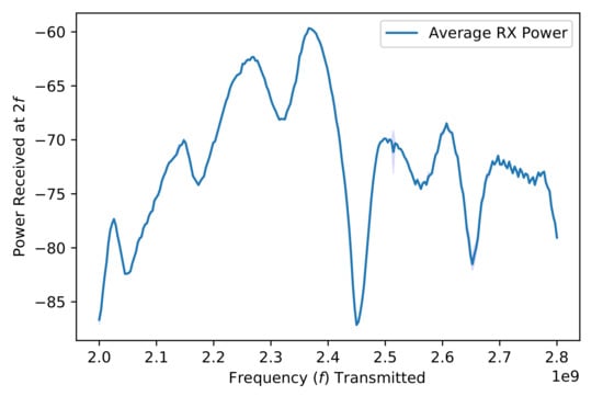
Figure 6.
Harmonic response for a laptop over a range of 800 MHz. Frequencies were tested in steps of 3.2 MHz. The values in the plot are an average of 5 readings.
6.2.2. Power
From the discussion of the experimental setup, we are interested in first describing the relationship between signal power input and output and then finding an appropriate power level for the experiments. Figure 7 presents the average received power of the harmonic () over 10 runs with the standard deviation highlighted. The linear fit of the data shows the intercept at −81.5295 and the slope of the line as 1.4542 with an of 0.997. Theoretically, while the expected return at the second harmonic is 2:1 with respect to the transmitted power, we accept these results as good approximations and as confirmation that our system is behaving as expected from the literature.
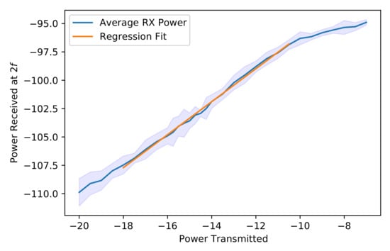
Figure 7.
Harmonic response with varying transmitted (input) signal power. Power levels were tested in steps of 0.5 dBm between −20 and −7 dBm.
Finally, we scanned over 5000 points to find the combination of power and frequency for the experiments. From Figure 6 we would expect the best results between 2.3 and 2.4 GHz, so we studied our working spectrum (2.0–2.8 GHz) to determine how variations in power affected the return signal. Figure 8 presents the readings collected. For all points collected, the noise floor was −91.699 dBm with a standard deviation of 2.277 dBm. Signals measured over 84 dBm indicate a successful detection. The strongest measurements occurred between 2.30 and 2.35 GHz, with the strongest among those correlating to higher transmit power. Not surprisingly, the selection of appropriate power settings is dependent on the target and the transmission channel. Furthermore, increasing the transmitted signal power also increased the noise in the system, because the signal generator and the spectrum analyzer are both electronic components and thus generate their own harmonics.
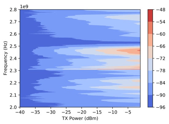
Figure 8.
Strength of the received harmonic signal (dBm) while varying power and frequency settings.
6.3. Wired Connection Results
For the wired testbed, in which the signal was transmitted by wire and fed directly into the circuit board of the target (Figure 2), each of the devices being tested were fitted with an SMA connector and connected through a coupler to the incoming and outgoing circuit.
We tested 12 devices (shown in Figure 4) in the wired configuration. Table 1 presents detailed results for each target and Figure 9 presents a visual comparison; the horizontal line shows where we set the threshold. We tested a combination of electronic, electric, and metallic targets. As the equivalent of a resistor in an RF circuit, the ‘dummy load’ is our baseline case. This object is a solid piece of metal, which should not (and did not) return a harmonic response. The light bulb, in this test, is a purely electric, filament model, with no electronics. (In Section 7, we compare the filament bulb with its Smart Light Bulb counterpart.)

Table 1.
Wired testbed results. The average noise level (floor) was −91.567 dBm with a standard deviation of 1.466 dB. Each measurement is an average of 15 readings with standard deviation shown in parenthesis.
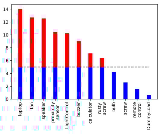
Figure 9.
Wired testbed: strength of the received harmonic signal for different targets. The horizontal line shows the threshold set at 5 dB. Targets with returned signal strength of over 5 dB were considered nonlinear (electronic).
Although these ‘wired’ experiments served to build confidence in the ability of the harmonic radar to detect electronics, these results are somewhat artificial. In a home environment, it is not practical to expect consumer electronics to have an SMA port available and for users to need to connect the device just to detect its presence. We thus proceed now to the wireless testbed and present the results obtained when the radio wave is transmitted over the air.
7. Wireless Testbed Results
The second testbed substitutes the coupler connecting the system with two antennas. Figure 3 presents the block diagram and Figure 10 presents a picture of one of the experiments. In the picture, the target is a laptop; the laptop is held vertical by two pieces of packing foam. For the detection experiment, the antennas and the target are placed forming a triangle with all sides measuring about 35 cm. We taped the antennas to the table to maintain a fixed separation and there is a cross section of the target device that is in the same plane as the antennas. (In future work, we may explore the effect of orientation on the received signal.) Each device was held in place by two sheets of packing foam material. We placed antennas and devices at a height of 73 cm from the floor.
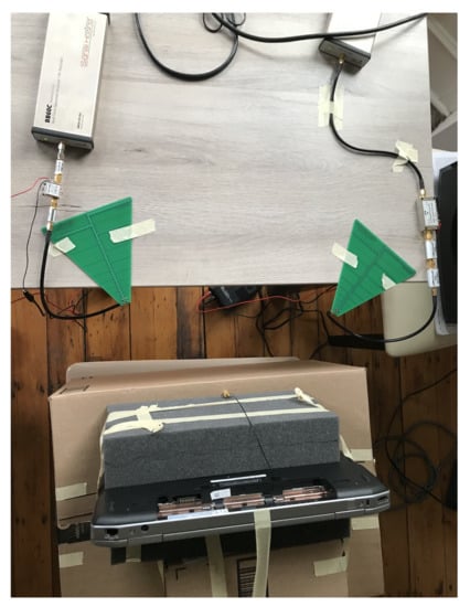
Figure 10.
Wireless testbed (top-down view). The target device here is a laptop held vertically by blocks of foam. The distance between the antennas is 30 cm. This picture corresponds to the results presented in Section 7.1 at a distance of 35 cm.
The experiments were carried out in a controlled home environment with the components fixed in position, but with people moving in the background and in neighboring apartments. Moreover, the testing environment had the normal RF noise that comes with a busy metropolitan location. These circumstances, instead of hindering the results, produce results comparable to what we might expect when our system is deployed in its intended environment: smart homes in normal operation.
Table 2 presents the output of the experiments in the wireless testbed. The column named Difference and the height of the bar in Figure 11 mark the received-signal-strength difference between measurements recorded when the device was present in the setup or not.
Table 2.
Wireless testbed results. The average noise level (floor) was −92.787 dBm with a standard deviation of 0.406 dB. Each measurement is an average of 15 readings with standard deviation shown in parenthesis.
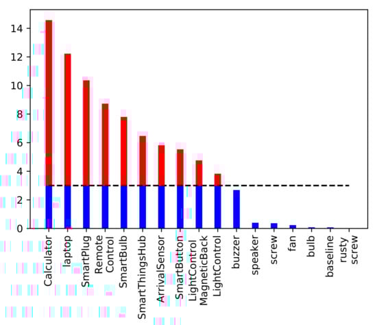
Figure 11.
Wireless testbed: strength of the received harmonic signal for different targets. The horizontal line shows the threshold set at 3 dB. Targets with returned signal strength of over 3 dB were considered nonlinear (electronic).
We present a total of 15 devices, shown in Figure 4, one of which was measured twice. From the picture we can see that there is great variety in terms of size, shape, and functionality. The Smart Light Control operates as a dimmer and a switch and is able to communicate wirelessly with a control application. The back of the device is magnetized so that it holds in place (and can be removed from) a metallic plate mounted on the wall (Figure 4i). We believe that both measurements are interesting to show. First both options are likely to happen in a Smart Home environment (think for example of a device that has been lost); and second it provides, like the empty baseline, a sanity check in terms of the results we are presenting.
The Outcome column in Table 2 as well as the dashed line in Figure 11 present the threshold for detection in this paper. For now, we manually selected the threshold based on the strength of the reflected signal and the expectation of nonlinearity from the target. One rule of thumb says that for a confident determination of detection, the received signal must be around 8 dB above the noise level. Following this convention, we could confidently identify four devices as electronic. This threshold would result in false negatives for all targets to the right of the Remote Control. Since we know the Light Control (with and without its magnetic backing) are electronic, the correct threshold would need to include them in the set, leaving the buzzer as borderline. Another direction for future work (discussed in Section 9) is in an adaptive algorithm that considers range and signal strength in its determination.
7.1. Distance, Power, and Near-Field Effects
Presented in Figure 12 is the harmonic response recorded from the laptop at distances ranging from 15 cm to 95 cm away from the Tx/Rx antennas, probed by a range of transmit powers (fed into the Tx antenna) ranging from −20 dBm to +5 dBm. Figure 13 is a colormap view of a subset of this data, for a slightly narrower range of transmit powers.
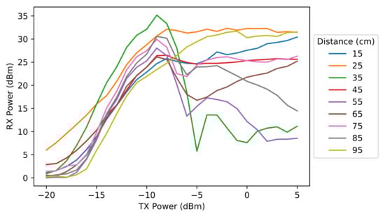
Figure 12.
Difference between transmitted and received signal strength for the laptop over three distances.
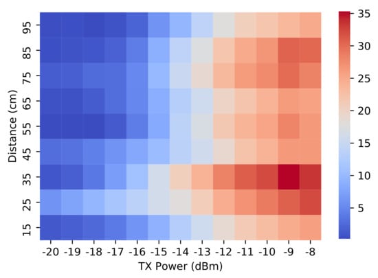
Figure 13.
Changes in power of the received signal signal for the laptop over a range of distances and transmitted power. In a gradient, deeper red indicates a stronger harmonic signal and deeper blue means the received signal was indistinguishable from noise.
Generally, with more RF power fed into the transmit antennas, more RF power is incident on the target, more harmonic is generated, and a stronger target response is received. However, for each target, there exists an input power level beyond which the nonlinearity (e.g., diode junction, transistor input) is maximally activated. In the context of magnetic cores for transformers or RF power amplifiers, this point is known as saturation: no additional field or power may be elicited from the device. In the context of nonlinear radar, no more harmonic may be reflected from the target. Furthermore, additional increases in power beyond the saturation point may cause other nonlinearities to activate, which reduce the harmonic reflected from the target. One possibility is that the incident RF power above saturation exceeds the breakdown voltage of the nonlinear junction generating the harmonic: before exceeding this threshold, the junction behaves like a diode following an exponential voltage/current profile such as modeled by Shockley’s equation and the harmonic tracks with a smooth slope (as seen in the −20 dBm to −10 dBm transmit-power range in Figure 12); after exceeding this threshold, the junction behaves more like a closed-switch/short-circuit that is minimally nonlinear (and might track like the 35-cm trace above −10 dBm transmit power in Figure 12).
Additionally, usually when the target is closer to the Tx/Rx antennas, the captured harmonic response is stronger. In the present study, however, all targets tested at all distances were within the near-field of the log periodic antennas. In the near-field, the RF power emitted by an antenna (and therefore incident on the target) does not necessarily follow the trend given by the classical Friis equation. The exact trend is calculated using a full set of Maxwell’s Equations for electric and magnetic fields, and those equations are tailored to the particular geometry of the antenna. It is still generally true that the power sent from an antenna is stronger closer to the antenna, but because of constructive and destructive interference in the fields emanating from each part of the antenna, there exist dips/nulls in the power-vs.-distance pattern within approximately 10 wavelengths. In Figure 12 and Figure 13, we observe that the harmonic response from the laptop was indeed generally stronger closer to the antennas and weaker farther away (i.e., the deepest red in Figure 13 appears at a distance of 35 cm, while the deepest blue appears at a distance of 95 cm). Because of near-field antenna properties, we observed the received-power-vs.-distance trend (vertically across Figure 13) was not monotonic, as expected. For a future experiment conducted in the far field (more than 10 wavelengths between the antennas and the target), we expect the received harmonic to decay with distance as as predicted by Equation (4).
8. Discussion
Finally, for the system to be adopted as a robust method for device detection, we must first address two remaining challenges. First, the automation of the threshold for detection. It is difficult to determine a consistent difference in thresholds between the wired results of Figure 9 and the wireless results of Figure 11. Take as an example the rusty screw. Back in the 1970s when nonlinear responses were first studied, metal oxides were (correctly) understood to reflect false positives. In our wired experiments, where the signal was fed directly into the screw, the response was indeed nonlinear. In the wireless experiments, however, at a distance of 12cm, the rusty screw was indistinguishable from the noise floor. The orientation of the screw might have an impact on the intensity of the response. We plan to explore this in future work.
Second, we are interested in a system that can potentially be used by non-experts in their home. The work presented here allows us to test the suitability of the technology for the purpose of detection. It is our belief that we presented experiments with encouraging results. One area that we did not address was the portability and ease of use for the system. In this stage of our work, that question is out of scope. However, in the future, if ongoing experiments continue to be encouraging, we will partner with colleagues from Electrical Engineering to develop a sensor that incorporates the principles we are using for detection.
9. Limitations and Future Work
We envision a system that can detect, fingerprint, and locate devices in room and we are proposing nonlinear junction detection (aka harmonic radars) as the technology that can help us achieve our goal. Taking each task as a separate project, we first build and test a device detection system that explores the harmonic response of traditional, electric, and electronic—regardless of their network capability, even if they are unplugged or powered off. In a sense, we are working towards developing a radar system for the home (complete with location and ranging capabilities). On the goal of detection, expansions of this work might include the number and variety of devices tested, measuring the response for different orientations per device, and testing the experimental limits (or range) in terms of distance between antenna and target. The choice of hardware components in the RF circuit also led to one of the first limitations we accepted, in this paper we only study a device’s response at the second harmonic. It is possible the combination of multiple harmonics could result in a distinct device signature.
In addition to the detection, identification, and ranging capabilities of the radar component, there is also room to grow in terms of the back-end and support systems that will be part of the final solution. In the motivating scenarios we presented, a common thread was the addition of dozens of devices to home environments. Therefore, while detecting all devices is essential, we are interested in alerting users to the presence of new, potentially unwanted, devices. For this, we need to create a repository of known devices and compare new signals against known signals; and alert and allow users to label new signals and guide them towards unwanted ones. As part of this same task, we need to expand this work to detect multiple instances of the same device (even if they are co-located). Finally, while at the moment we are manually selecting the threshold that separates ’electronics’ from ‘others’ (i.e., the dashed line in Figure 9 and Figure 11), in time, we hope to incorporate semi-supervised learning algorithms to automatically set this parameter.
10. Conclusions
We explored the possibility of using harmonic radar to discover consumer electronics inside the home. We tested a set of 16 distinct devices (or objects) and showed that the electronic devices were detectable at distances ranging from 15 cm to 1 meter at different power levels. From the literature, we know that harmonic-radar technology can work over a range of hundreds of feet, leaving open the potential for this approach to be effective on a house-wide scale.
Two major benefits of the harmonic-radar approach are that (1) the devices can be detected even powered off, with the battery removed, and (2) the method is agnostic to the communication technology used by the target device—even if the device never communicates at all.
We continue to explore this technology to determine what other benefits it might bring to privacy-preserving smart-home technologies.
Author Contributions
Conceptualization, T.J.P. and D.K.; data curation, B.P.; formal analysis, G.M.; funding acquisition, T.J.P. and D.K.; investigation, B.P.; methodology, B.P., G.M. and T.J.P.; project administration, D.K.; resources, T.J.P. and D.K.; supervision, G.M. and D.K.; validation, D.K.; writing—original draft, B.P., G.M. and T.J.P.; writing—review and editing, G.M., T.J.P. and D.K.. All authors have read and agreed to the published version of the manuscript.
Funding
This work is supported by he U.S. National Science Foundation under grants 1955805 (SaTC Frontiers program) and 2030859 (the Computing Research Association for the CIFellows Project).
Conflicts of Interest
The authors declare no conflict of interest.
References
- Wikipedia. Amazon Echo. 2019. Available online: https://en.wikipedia.org/wiki/Amazon_Echo (accessed on 25 October 2021).
- Wikipedia. Google Home. 2019. Available online: https://en.wikipedia.org/wiki/Google_Home (accessed on 25 October 2021).
- Signify Holding. Smart Mood Lighting. 2021. Available online: https://www.philips-hue.com/en-us/explore-hue/propositions/personal-mood-lighting (accessed on 25 October 2021).
- Yale, ASSA ABLOY Residential Group. Smart Door Locks; Yale, ASSA ABLOY Residential Group: Stockholm, Sweden, 2021. [Google Scholar]
- Samsung. Smart Refrigerator. 2021. Available online: https://www.samsung.com/us/explore/family-hub-refrigerator/overview/ (accessed on 25 October 2021).
- McKinsey & Company. Growing Opportunities in the Internet of Things; McKinsey & Company: San Francisco, CA, USA, 2021. [Google Scholar]
- Moy de Vitry, M.; Schneider, M.Y.; Wani, O.F.; Manny, L.; Leitão, J.P.; Eggimann, S. Smart urban water systems: What Could possibly go wrong? Environ. Res. Lett. 2019, 14, 081001. [Google Scholar] [CrossRef]
- Sami, S.; Dai, Y.; Tan, S.R.X.; Roy, N.; Han, J. Spying with your robot vacuum cleaner: Eavesdropping via lidar sensors. In Proceedings of the ACM Conference on Embedded Networked Sensor Systems (Sensys), Virtual, 16–19 November 2020; pp. 354–367. [Google Scholar]
- Mazzaro, G.J.; Gallagher, K.A.; Sherbondy, K.D.; Martone, A.F. Nonlinear radar: A historical overview and a summary of recent advancements. Proc. SPIE 2020, 11408, 114080E. [Google Scholar]
- Pedro, J.C.; Carvalho, N.B. Intermodulation Distortion in Microwave and Wireless Circuits; Artech House: Norwood, MA, USA, 2003. [Google Scholar]
- Gallagher, K. Harmonic Radar: Theory and Applications to Nonlinear Target Detection, Tracking, Imaging and Classification. Ph.D. Thesis, Pennsylvania State University, State College, PA, USA, 2015. [Google Scholar]
- Martone, A.F.; Ranney, K.I.; Sherbondy, K.D.; Gallagher, K.A.; Mazzaro, G.J.; Narayanan, R.M. An overview of spectrum sensing for harmonic radar. In Proceedings of the 2016 International Symposium on Fundamentals of Electrical Engineering (ISFEE), Bucharest, Romania, 30 June–2 July 2016; pp. 1–5. [Google Scholar] [CrossRef]
- Viikari, V.; Kantanen, M.; Varpula, T.; Lamminen, A.; Alastalo, A.; Mattila, T.; Seppa, H.; Pursula, P.; Saebboe, J.; Cheng, S.; et al. Technical solutions for automotive intermodulation radar for detecting vulnerable road users. In Proceedings of the VTC Spring 2009-IEEE 69th Vehicular Technology Conference, Barcelona, Spain, 26–29 April 2009; pp. 1–5. [Google Scholar]
- Aumann, H.M.; Emanetoglu, N.W. A wideband harmonic radar for tracking small wood frogs. In Proceedings of the 2014 IEEE Radar Conference, Cincinnati, OH, USA, 19–23 May 2014; pp. 0108–0111. [Google Scholar]
- Tsai, Z.M.; Jau, P.H.; Kuo, N.C.; Kao, J.C.; Lin, K.Y.; Chang, F.R.; Yang, E.C.; Wang, H. A high-range-accuracy and high-sensitivity harmonic radar using pulse pseudorandom code for bee searching. IEEE Trans. Microw. Theory Tech. 2012, 61, 666–675. [Google Scholar] [CrossRef]
- Kim, J.; Jung, M.; Kim, H.G.; Lee, D.H. Potential of harmonic radar system for use on five economically important insects: Radar tag attachment on insects and its impact on flight capacity. J. Asia-Pac. Entomol. 2016, 19, 371–375. [Google Scholar] [CrossRef]
- Aballo, T.; Cabria, L.; Garcia, J.; Fernandez, T.; Marante, F. Taking advantage of a Schottky junction nonlinear characteristic for radiofrequency temperature sensing. In Proceedings of the 2006 European Microwave Conference, Manchester, UK, 10–15 September 2006; pp. 318–321. [Google Scholar]
- Kubina, B.; Romeu, J.; Mandel, C.; Schüßler, M.; Jakoby, R. Design of a quasi-chipless harmonic radar sensor for ambient temperature sensing. In Proceedings of the 2014 IEEE SENSORS, Valencia, Spain, 2–5 November 2014; pp. 1567–1570. [Google Scholar]
- Harzheim, T.; Mühmel, M.; Heuermann, H. A SFCW harmonic radar system for maritime search and rescue using passive and active tags. Int. J. Microw. Wirel. Technol. 2021, 13, 1–17. [Google Scholar] [CrossRef]
- Fussell, S. Airbnb Has a Hidden Camera Problem. 2019. Available online: https://www.theatlantic.com/technology/archive/2019/03/what-happens-when-you-find-cameras-your-airbnb/585007/ (accessed on 25 October 2021).
- Kaddoum, G. Wireless Chaos-Based Communication Systems: A Comprehensive Survey. IEEE Access 2016, 4, 2621–2648. [Google Scholar] [CrossRef]
- Cabrera, C.; Palade, A.; Clarke, S. An Evaluation of Service Discovery Protocols in the Internet of Things. In Proceedings of the Symposium on Applied Computing (SAC), Marrakech, Morocco, 4–6 April 2017; pp. 469–476. [Google Scholar]
- Aniktar, H.; Baran, D.; Karav, E.; Akkaya, E.; Birecik, Y.S.; Sezgin, M. Getting the bugs out: A portable harmonic radar system for electronic countersurveillance applications. IEEE Microw. Mag. 2015, 16, 40–52. [Google Scholar] [CrossRef]
- Mazzaro, G.J.; Sherbondy, K.D. Filter Selection for Wideband Harmonic Radar. In Proceedings of the 2019 SoutheastCon, Huntsville, AL, USA, 11–14 April 2019; pp. 1–6. [Google Scholar]
- Colpitts, B.G.; Boiteau, G. Harmonic radar transceiver design: Miniature tags for insect tracking. IEEE Trans. Antennas Propag. 2004, 52, 2825–2832. [Google Scholar] [CrossRef]
- Kiriazi, J.; Nakakura, J.; Hall, K.; Hafner, N.; Lubecke, V. Low Profile Harmonic Radar Transponder for Tracking Small Endangered Species. In Proceedings of the 2007 29th Annual International Conference of the IEEE Engineering in Medicine and Biology Society, Lyon, France, 22–26 August 2007; pp. 2338–2341. [Google Scholar] [CrossRef]
- Kim, I.H.; Min, K.S.; Jeong, J.H.; Kim, S.M. Circularly polarized tripleband patch antenna for non-linear junction detector. In Proceedings of the 2013 Asia-Pacific Microwave Conference Proceedings (APMC), Seoul, Korea, 5–8 November 2013; pp. 140–142. [Google Scholar] [CrossRef]
- Gallagher, K.A.; Mazzaro, G.J.; Martone, A.F.; Sherbondy, K.D.; Narayanan, R.M. Derivation and validation of the nonlinear radar range equation. Proc. SPIE 2016, 9829, 98290P. [Google Scholar]
- Gallagher, K.A.; Narayanan, R.M.; Mazzaro, G.J.; Ranney, K.I.; Martone, A.F.; Sherbondy, K.D. Moving target indication with non-linear radar. In Proceedings of the 2015 IEEE Radar Conference (RadarCon), Arlington, VA, USA, 10–15 May 2015; pp. 1428–1433. [Google Scholar] [CrossRef]
- Ilbegi, H.; Hayvaci, H.T.; Yetik, I.S.; Yilmaz, A.E. Distinguishing electronic devices using harmonic radar. In Proceedings of the 2017 IEEE Radar Conference (RadarConf), Seattle, WA, USA, 8–12 May 2017; pp. 1527–1530. [Google Scholar] [CrossRef]
- Mazzaro, G.; Gallagher, K.; Sherbondy, K.; Salik, K. Detecting Nonlinear Junctions Using Harmonic Cross-Modulation. In Proceedings of the SoutheastCon 2021, Atlanta, GA, USA, 10–13 March 2021; pp. 1–7. [Google Scholar]
- Singh, A.; Lubecke, V.M. Respiratory monitoring and clutter rejection using a CW Doppler radar with passive RF tags. IEEE Sens. J. 2011, 12, 558–565. [Google Scholar] [CrossRef]
- Mazzaro, G.J.; Sherbondy, K.D. Harmonic nonlinear radar: From benchtop experimentation to short-range wireless data collection. In Radar Sensor Technology XXIII; Ranney, K.I., Doerry, A., Eds.; International Society for Optics and Photonics, SPIE: San Diego, CA, USA, 2019; Volume 11003, pp. 91–101. [Google Scholar] [CrossRef]
- Gorbatenko, N.N.; Semenikhina, D.V. A radiation characteristic of perfect conducted cylinder with non-linear loads covered with a layer of metematerial. In Proceedings of the 2018 IEEE Conference of Russian Young Researchers in Electrical and Electronic Engineering (EIConRus), Moscow and St. Petersburg, Russia, 29 January–1 February 2018; pp. 465–467. [Google Scholar]
- Mazzaro, G.J.; Martone, A.F.; Sherbondy, K.D.; Gallagher, K.A.; Narayanan, R.M. Maximizing harmonic-radar target response: Duty cycle vs. peak power. In Proceedings of the SoutheastCon 2016, Norfolk, VA, USA, 30 March–3 April 2016; pp. 1–4. [Google Scholar]
- Signal Hound. VSG60A—6 GHz Vector Signal Generator. 2021. Available online: https://signalhound.com/products/vsg60a-6-ghz-vector-signal-generator/ (accessed on 25 October 2021).
- Signal Hound. BB60C—6 GHz Real-time Spectrum Analyzer. 2021. Available online: https://signalhound.com/products/bb60c/ (accessed on 25 October 2021).
- Mazzaro, G.J.; Martone, A.F.; McNamara, D.M. Detection of RF electronics by multitone harmonic radar. IEEE Trans. Aerosp. Electron. Syst. 2014, 50, 477–490. [Google Scholar] [CrossRef]


Publisher’s Note: MDPI stays neutral with regard to jurisdictional claims in published maps and institutional affiliations. |
© 2022 by the authors. Licensee MDPI, Basel, Switzerland. This article is an open access article distributed under the terms and conditions of the Creative Commons Attribution (CC BY) license (https://creativecommons.org/licenses/by/4.0/).