Earth Observation via Compressive Sensing: The Effect of Satellite Motion

Abstract

In the framework of earth observation for scientific purposes, we consider a multiband spatial compressive sensing (CS) acquisition system, based on a pushbroom scanning. We conduct a series of analyses to address the effects of the satellite movement on its performance in a context of a future space mission aimed at monitoring the cryosphere. We initially apply the state-of-the-art techniques of CS to static images, and evaluate the reconstruction errors on representative scenes of the earth. We then extend the reconstruction algorithms to pushframe acquisitions, i.e., static images processed line-by-line, and pushbroom acquisitions, i.e., moving frames, which consider the payload displacement during acquisition. A parallel analysis on the classical pushbroom acquisition strategy is also performed for comparison. Design guidelines following this analysis are then provided.

1. Introduction

Imaging spectroscopy is an effective tool, whose use is growing enormously in recent years, able to acquire not only spatially, but also spectrally resolved images. A multispectral or hyperspectral image is in fact a volumetric imagery dataset, consisting of a spatial array of optical spectra, sampled from contiguous wavelength channels. Among all the application fields [1,2,3,4,5,6], remote sensing and earth observation are taking advantage especially of the hyperspectral acquisition in the visible, near-infrared (NIR), short-wave (SWIR), and thermal infrared (TIR) spectrum, since the large spectral resolution of the resulting imagery allows teasing out the various materials composing the investigated surface [7]. In fact, nowadays, several space missions equipped with hyperspectral sensors are orbiting earth, which are devoted to different applications encompassing land, ocean, and atmospheric components [8,9,10,11,12,13,14].

In this framework, there is a strong driving force of finding new and alternative acquisition techniques with the idea of simplifying in size and complexity the acquisition hardware and the amount of data to be collected and transferred. A possibility is given by the work of the mathematicians Candes, Romberg, Tao, Donoho, and Baraniuk, who developed the compressive sensing (CS) technique [15,16,17,18,19,20,21]. They stated that, when a signal is of sparse nature, it could be sensed with a limited number of bases, well below the requirement of the Nyquist-Shannon theorem of sampling. Usually, remote sensing data compression is performed after the signal acquisition, as a requirement to reduce the amount of data to be transferred to earth. On the contrary, CS applies linear projections in the optical domain such that this dimensionality reduction occurs simultaneously with image sensing and acquisition. This brings about the capability of reducing the sampling operations at the sensory level, with the counterbalance of a computation effort in retrieving the original information [17,22]. After the demonstration of the single-pixel camera (SPC) in a restricted wavelength band [23], different architectures have been studied and prototyped [24], which exploit CS in either the spatial domain [3,25,26,27], the spectral domain [28,29,30,31], or both [32], to acquire multispectral or hyperspectral still images or movies [33,34]. These approaches usually consider the so-called framing acquisition, where the scene is fixed and imaged at once. The CS strategy has been shown to deliver good results, since the bases set and the reconstruction algorithms have been extensively developed.

In remote-sensing applications, a few examples of CS sensing architectures are reported in the literature [35,36,37,38]. Given the peculiar motion of the sensing platform, the whiskbroom (WB) or pushbroom (PB) acquisition strategies are the most suited. Conceptual designs exploiting CS in the spectral domain to sense hyperspectral images have been proposed [35,37]. In this case, the linear field of view is dispersed, the masks applied in the dispersed image plane, and the spectrally integrated light is focalized on a linear array. Here, the mask resolution limits the spectral resolution, while the spatial resolution is set by the detector pixel size. A first prototype of a pushframe camera exploiting the CS in the spatial domain has been recently reported [38], where the acquisition of moving scenes is performed with parallelized SPCs and an RGB detector. This approach has the advantage of a reduced acquisition time with respect to the classical SPC, but allows to acquire only multispectral images. A pushbroom hyperspectral device has also been reported to record static images, where the slit is moved across the field of view and CS performed within the single image slice [39].

The long acquisition time required to capture the image, which is the main limitation of SPCs, can be easily overcome in laboratory systems, where the exposure time and the resolution can be adapted to fit the available hardware. Conversely, in space observations, the rapid motion of a satellite across the earth restricts the exposure time, which is limited in image smear caused by the earth moving across one ground sampling distance. In fact, the dwell time (the time a sensor element covers one sampling distance) is set by the platform characteristics, which depend on the ground velocity and the ground resolution. As the spatial resolution increases with the number of patterns, for a given dwell time higher spatial resolution requires reducing the exposure time per pattern, with degradation of image quality or infeasibility. Considerations on the dwell time in CS have been seldom reported in the literature [35,38], even if they are strongly linked to the technological feasibility of these systems. On top of this, the performances of CS reconstruction in case of pushbroom acquisitions have usually been estimated with static images only, where the effect of the motion has been adapted to the experimental purposes [38].

The novelty of our approach consists in the evaluation of the performances of state-of-the-art compressive sensing methods to a pushbroom acquisition system for earth observation, not limited to image recognition but devoted to scientific purposes, as the precise measurement of the earth radiance in a large spectral window. In the direction suggested by [40], it is worth to test the CS method in any specific application: this work is useful to highlight possible intrinsic drawbacks of the CS technique and is propaedeutic for its technical improvement. In fact, no performance analyses of a pushbroom CS acquisition system are present in the literature, when performed under severe time constrains, represented by the intrinsic motion of the satellite and by the technological limitations of the available mask modulators.

Our framework is the design of a hyperspectral pushbroom CS acquisition system for earth observation, devoted to the analysis of the cryosphere in fragmented basins, as the Alps, the Asia High Mountains, and the Andes. Our benchmark is a very accurate determination of the surface albedo and temperature, fundamental to retrieve the snow thermal inertia and, eventually, the density of the snowpack [41]. We are dealing with an accuracy on the estimation of the earth radiance in the visible and thermal bands below a few percent RMS. On top of the spatial requirements (resolution of 20–80 m and swath of 100 km), a temporal requirement is necessary to retrieve the thermal inertia of the snowpack, of at least two daily acquisitions over the same area. This revisiting requirement is well beyond the possibility offered by any hyperspectral missions orbiting the earth at present.

In this respect, the development of alternative acquisition techniques may open the way to future space missions devoted to the study of the earth. CS may represent a valid solution to allow for low-cost hyperspectral imaging in the visible, infrared, and thermal regions, where pixelated sensors are limited in size and number of pixels, or available at a prohibitive price. In fact, linear sensors are sufficient to register hyperspectral images, since the spatial (or spectral) dimension is retrieved with CS. A clever optical design may also limit the dimensions of the spectroscopic arm of the payload, limiting the overall system volume. In this way, such payloads, mounted on small satellites working in constellation, may overcome the temporal resolution limitation characterizing the present orbiting missions, by preserving their spatial and spectral characteristics. However, this possibility passes through the demonstration of the effectiveness and accuracy of the pushbroom compressive sensing acquisition method with respect to the classical approach.

Accordingly, we extended the available CS reconstruction algorithms [42] to static images processed line-by-line to start mimicking the CS pushbroom method, and we simulated the acquisition of dynamic images via the compressive sensing pushbroom method, taking into account the payload motion during acquisition. A parallel analysis on the classical pushbroom (PB) acquisition strategy was performed for comparison. All the analysis started from multispectral images of mountainous regions covered with snowpack, acquired by the Landsat 8 space mission. Following the simulation results, we will provide guidelines on the acquisition strategy and on the related parameters when very high precision measurements are required.

2. Materials and Methods

The theory of CS applied to image reconstruction foresees that an image of $N$ pixels can be stored and then mathematically reconstructed by $M<N$ measurements, overcoming the limit of the cardinal theorem of interpolation. Although a complete treatment of the CS theory is beyond our purpose, we will introduce some key concepts, which are important to better understand the following paragraphs (for a deeper treatment the reader can refers to [21]).

Let us consider the signal to be acquired as a vector $x$ (in the case of an image matrix, its pixels are rearranged in a 1D vector). It can be decomposed into a base ${\left\{{\psi }_i\right\}}_{i=1}^N$ as $x={\displaystyle \sum }_i^N{s}_i{\psi }_i$ or, in matrix form,

$$x=\Psi s$$

(1)

where $s$ is the vector of the coefficients. Now we suppose to take $M<N$ measurements of the vector $x$, and, considering the measurement matrix $A$, we will end up with a measurement vector $y=Ax$, with just $M$ entries. Finally, we can write

$$y=A\Psi s=\Theta s$$

(2)

Finding $x$ from the measurement vector $y$ is an “ill-conditioned” problem, but the CS theory states that if $x$ is sparse in the $s$ decomposition or at least “compressible” (the intensity of the coefficients $s_i$ follows a fast decay [17]) it is possible to find a solution with a high accuracy even when $M\ll N$. The sparser is the image, the lower is the number of measurements needed to perform a quasi-perfect reconstruction. Basically, the problem is to find the sparsest solution which solve the equation. This can be done applying different algorithms, some of the most used are: ${\ell }_1$ minimization, greedy algorithm, or total variation (TV) minimization [15,19,42,43]. In the framework of image reconstruction, TV minimization and its optimized version called “TVAL3 solver” have been proved to be the most efficient in recovering the signals [42]. The TVAL3 solves the equation rewriting the problem as an augmented Lagrangian function, in its simpler form we have:

$$\underset{x}{\min }{\displaystyle \sum }_i\Vert D_{i}x\Vert s.t. Ax=y$$

(3)

where $D_{i}x$ denotes the discrete gradient vector of x at the i-th position and D is the gradient operator. The TVAL3 solver is available in a “ready to use” Matlab library, shared by the authors of [42].

Concerning the choice of the measurement matrix $A$, we consider three different possibilities: discrete cosine transform (DCT)-based matrices [44], Hadamard (HD) matrices [45], and an ordered version of the Hadamard matrices called “cutting cake” (CC) [46].

In the DCT case, the measurement vector $y$ is obtained from $M$ rows of a DCT matrix after a random permutation of its rows and columns. The measurement matrix is grayscale, which is a complication from a practical point of view, since digital micromirror devices (DMDs), which are intrinsically binary, are usually considered to produce the measurement masks.

In the Hadamard case, the measurement vector $y$ is obtained from $M$ random rows of a Hadamard matrix after a random permutation of its rows and columns. Here, the measurement matrices have entries which are +1 or −1, meaning that for each mask, the acquisition process must be done in two steps: one with a mask corresponding to the +1 pattern, and one with a mask corresponding to the −1 pattern; after that the two measures are subtracted to obtain the final result. By means of the DMD as mask generator, the +1 and −1 patterns may be acquired simultaneously, exploiting the two tilt positions of the DMD, using two identical reading channels. Differently from the classic HD, the CC algorithm applies a smart ordering, the so called cutting cake order. With such strategy, the measurement matrices, constructed from each row of the ordered Hadamard, have an increasing number of connected areas (i.e., an increased complexity). For a natural image, it has been demonstrated that the entries of the measurements vector $y,$ properly ordered, follow a fast decreasing curve [46,47], thus, in principle, the same reconstruction quality is obtained with a lower $M/N$, losing only the local image details. However, the ordering algorithm makes the reconstruction process more time consuming. This principle may be exploited for a “direct” CC reconstruction method. In fact, given that the reordering strategy of the CC algorithm ensures that the entries of the $y$ vector, which are the coefficients correspondent to each measurements matrix ${\psi }_i$, follow a perfect power decay, the optimization process to recover the image $x$ is in principle not required, because the most important components of the decomposition are already known. Thus, x can be recovered by simply applying $x^{\ast }={{\displaystyle \sum }}_{i=1}^M{\psi }_i{y}_i$, where the asterisk means the reconstruction is intrinsically incomplete, since $M<N$. Of course, in case of real images, this may not be completely true, and the reconstruction performances must be carefully characterized.

We considered as raw frames representative Level−1 data of the Landsat 8 mission [48,49], taken over fragmented areas as mountains and valleys (Figure 1). Images are available at different wavelength bands (from the visible to the TIR, see

Table 1. Parameters of the Landsat 8 data considered in our simulations.

Channel	Wavelength (µm)	Resolution (m)
2	0.450–0.515	30
3	0.525–0.600	30
4	0.630–0.680	30
5	0.845–0.885	30
10	10.600–11.200	100

for details), with an earth resolution of 30 m or 100 m.

3. Results

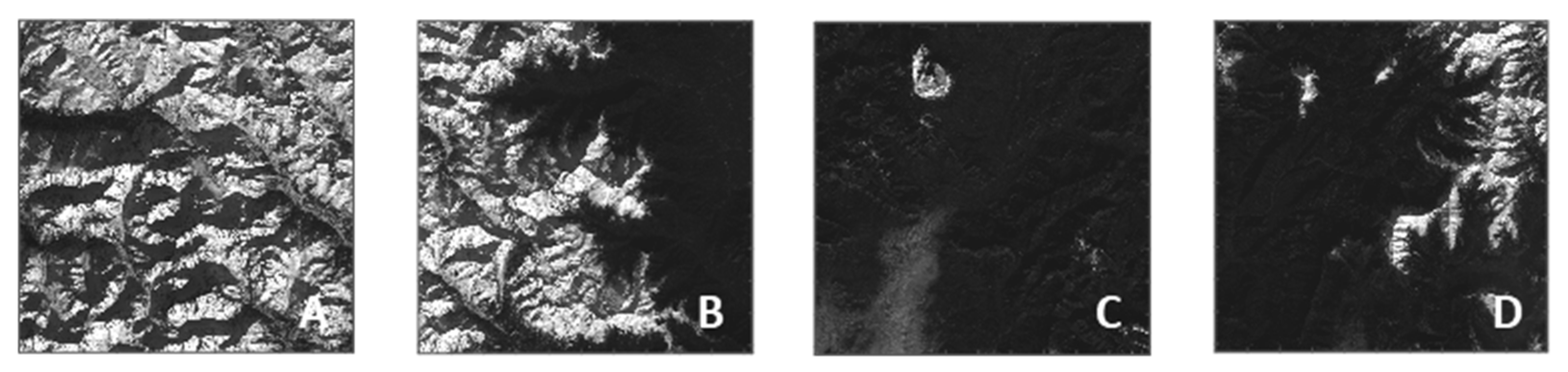
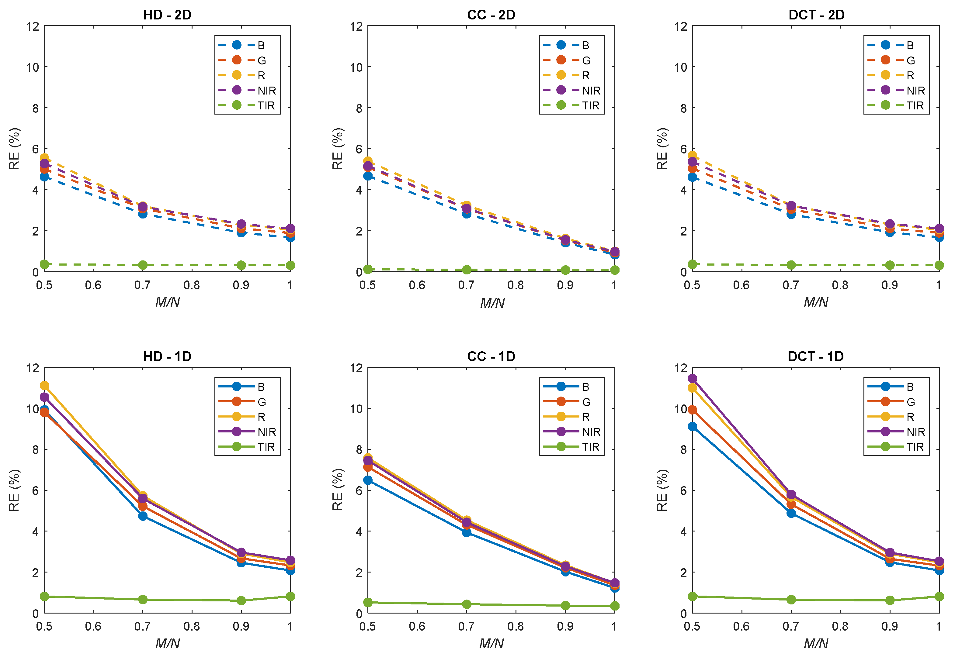
3.1. Reconstruction Performances of Static Images

Before considering moving images, and setting a term of comparison, we evaluate the CS reconstruction performances of static images. For each channel, we apply the reconstruction process on five images with two different methodologies, that we call 2D and 1D. The 2D method is the classical approach, where the image is reconstructed as a whole. In the 1D approach, the images are divided in vertical stripes, one pixel wide, reconstructed as independent measurements, and concatenated afterwards to give the whole image. No filters are applied between the stripes.

Three basis set have been chosen to build up the measurement matrix A, the so called DCT, HD, and CC. $M/N$, also called $\rho ,$ is the ratio between the number of mask $M$ and the number of pixel $N$ which is used to build the measurement vector $y$; ${\sigma }_{noise}$ is the amount of Gaussian noise artificially introduced in the vector $y$ to simulate a real acquisition process.

Table 2. Simulation parameters.

Simulation Parameters
Channel	R, G, B, NIR, TIR
Basis set	DCT; HD; CC
Reconstruction method	TVAL (1D–2D); direct (1D–2D)
$\rho =M/N$	0.1; 0.3; 0.5; 0.7; 0.9; 1
${\sigma }_{noise}$	0%; 5%

summarizes all the parameters, explored in the simulations.

We considered the reconstruction error (RE) as the figure of merit [46]

$$RE \left(\%\right) =\frac{\Vert \tilde{u}-u_0\Vert {}_F}{\Vert u_0\Vert {}_F}\times 100$$

(4)

where $\tilde{u}$ denotes the reconstructed image and $u_0$ stands for the original image. Here, $\Vert u\Vert {}_F$ is called Frobenius norm which can be defined as

$$\Vert u\Vert {}_F=\sqrt{{\displaystyle \sum }_{i=1}^q{\displaystyle \sum }_{j=1}^p{\left|u_{ij}\right|}^2}$$

(5)

Among the different criteria to evaluate the reconstruction quality, such as the peak signal-to-noise ratio (PSNR) or the structural similarity index measure (SSIM), the RE gives a direct quantification of the average error over the image. On the other hand, the PSNR and the SSIM are commonly used to evaluate the perceived quality of the image.

The reconstruction quality in terms of RE of a representative image (box A, Figure 1) is reported in Figure 2 for the different basis sets and for both the 2D and 1D processes. In 2D, the trends are all comparable, while in 1D the Hadamard-based methods, and the CC in particular, give smaller reconstruction errors than the DCT, especially at low $M/N$.

In all cases, the 1D reconstruction process is always less accurate than the 2D. Concerning the dependence on the ratio $M/N$, when the number of measurements approaches the number of pixels, the reconstruction error decreases, since the reconstruction basis is more complete. In these simulations, we always consider a noise error of 5%, which is the reason why the RE never reaches zero even when all the masks are applied. However, there is a huge difference between the channels: in the TIR case, the error is always low, generally below 1%, while in the visible the RE is much higher and reaches values of 1–3% only for high values of $M/N$, generally higher than 0.8.

Figure 3 reports the reconstruction errors of the same image in three different spectral bands (B, NIR, TIR), with a level of noise of 0% and 5%, as function of the reconstruction methods: in particular, we consider the CC basis, with the TVAL or the direct reconstruction methods. The difference between the TVAL-CC and direct-CC is not severe, especially when $M/N$ is large, indicating that the CC is effective in ordering the most important basis. Therefore, the choice between the two methods mainly depends on the computational time available; in fact, avoiding the TVAL optimization reduces the post processing time of one order of magnitude. Moreover, in this case we observe a difference between the channels: the RE for visible channels shows a decreasing linear trend with $M/N$ between 0.5 and 1, while for the TIR channel, especially when ${\sigma }_{noise}=0$, the trend is less steep, with a fast decay after $M/N=0.9$.

To generalize these evidence, we hereafter extend the reconstruction simulations on a larger sample of images of the Alps, under different conditions. Figure 4 shows, in four representative cases (A–D), the comparison between the G and TIR images, where column A represents the case of mountains covered by snow, columns B and C represent mountains without snow, and column D, a portion covered by clouds. For each one, we perform the simulated acquisition and reconstruction with the CC-direct method and ${\sigma }_{noise}=0$.

On the bottom line we report the reconstruction errors for all the channels, and it is clear that the recovery efficiency is directly related to the scene under study. For example, scene D (clouds) is by far the best reconstructed one, while scene A (mountains with snow) is the worst. In any case, we observe a large difference between the reconstruction performances in the various channels, especially at low $M/N$ values. The TIR channel is always the best reconstructed and, in the visible region, the reconstruction performances improve at smaller wavelengths. These discrepancies rely on the different morphological features highlighted in the different channels and the reconstruction efficiency depends on the sparsity of the images. The third line of Figure 4 reports the entries of the vector $s$ (Equation (1)), obtained projecting the image on each basis used for reconstruction, for the G and TIR channels. The masks ordering follows the CC order. When the intensity of the vector $s$ is concentrated in few masks, i.e., the image is sparser in the basis set (more compressible) and fewer masks are necessary to reconstruct the image with low RE (see case D). In analogy, when the intensity distribution of the vector $s$ is similar in the two channels, the corresponding REs are comparable (see case B), since they show a similar compressibility. Finally, the larger is the difference in the intensity distribution of the vector $s$ between the channels, the larger is the difference in the REs (see cases A and C). This is due to the morphological features of the images, which vary inside our set of images. In any case, the RE reduces when a larger number of masks is used for the reconstruction, and, for ${\sigma }_{noise}=0,$ becomes null when the basis set is complete, i.e., when $M=N$.

In conclusion, this behavior indicates that, even if the images are of the same nature, the reconstruction error depends on the single frame, and larger accuracies can be obtained only for an almost complete basis set.

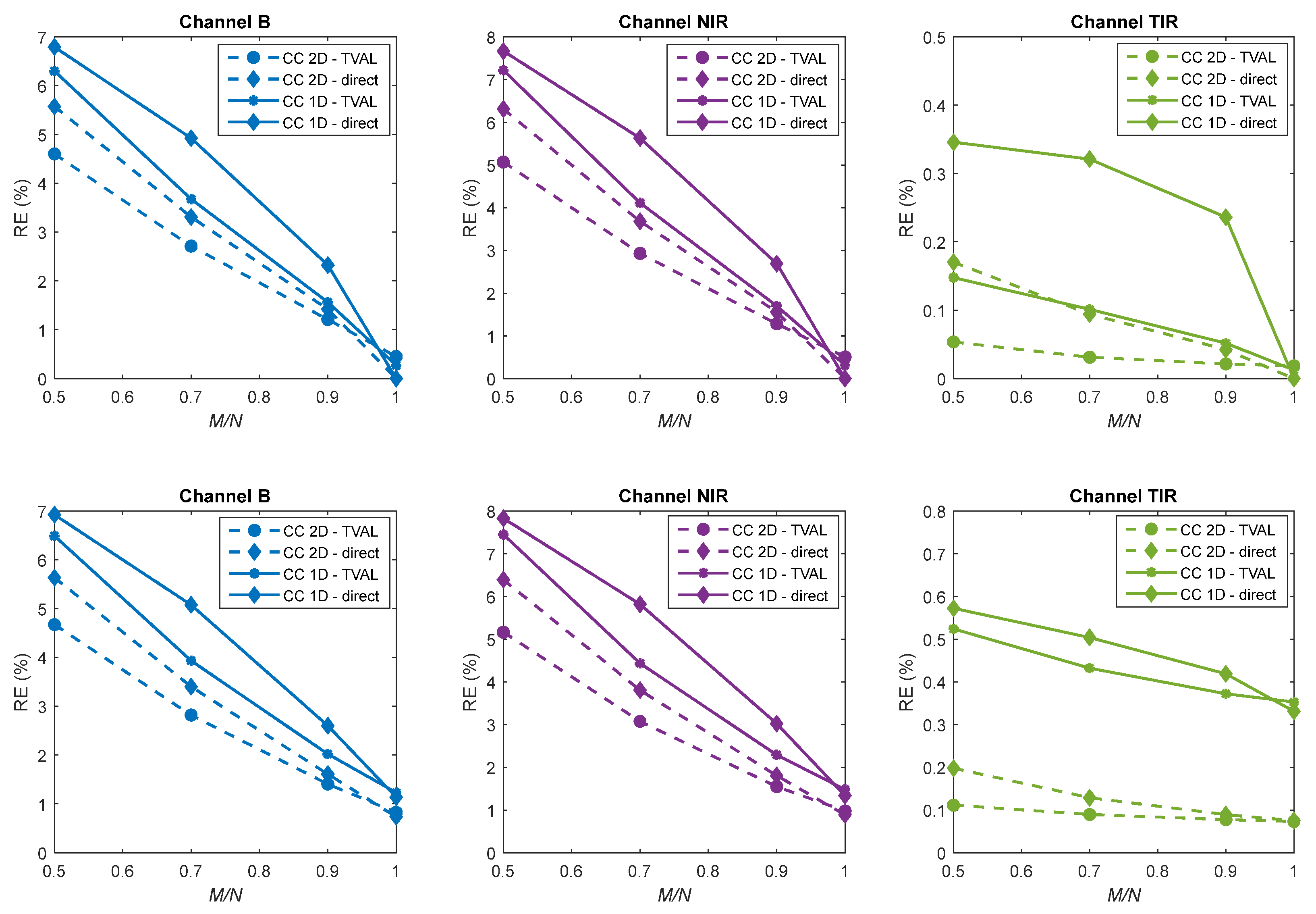
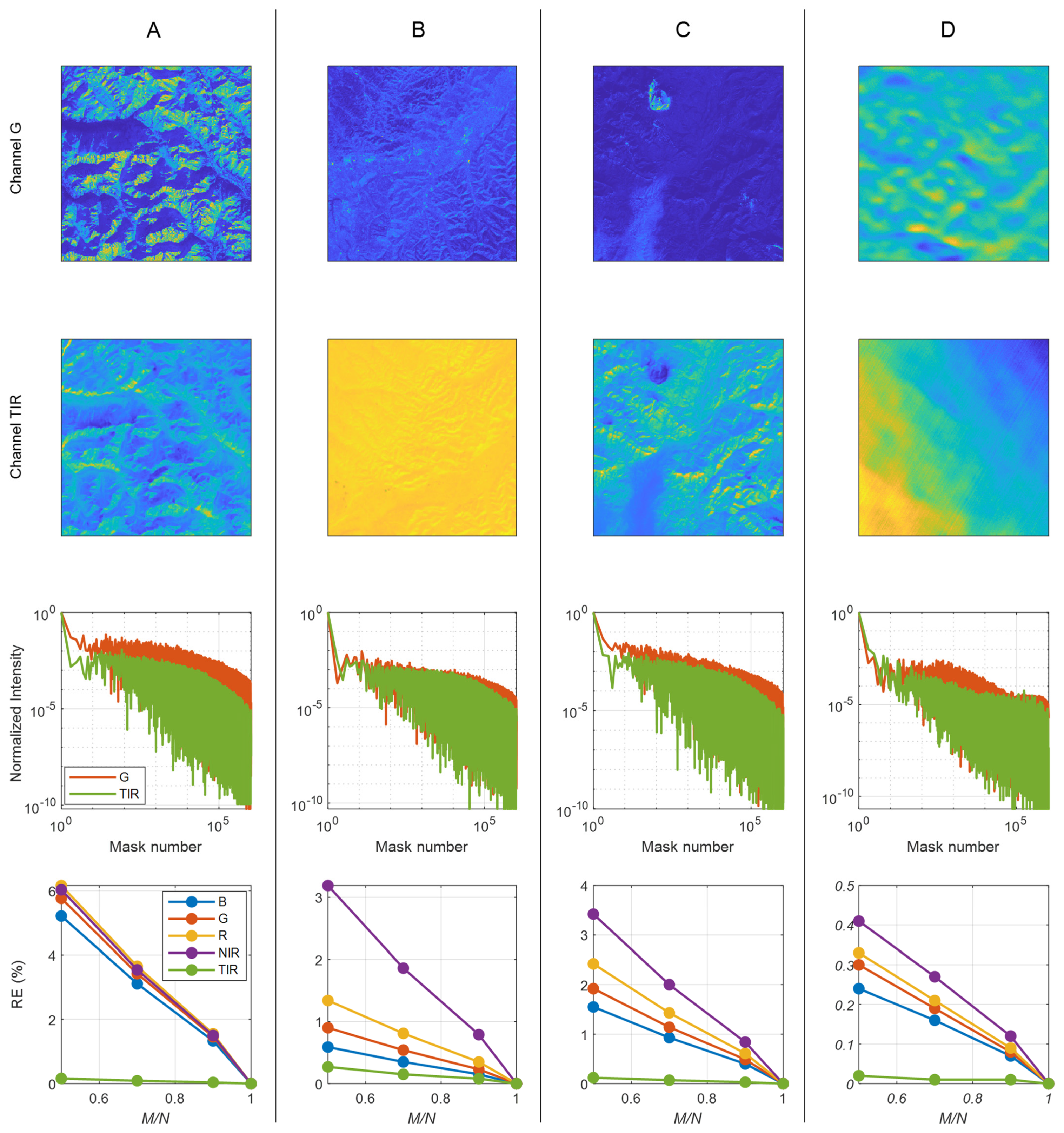
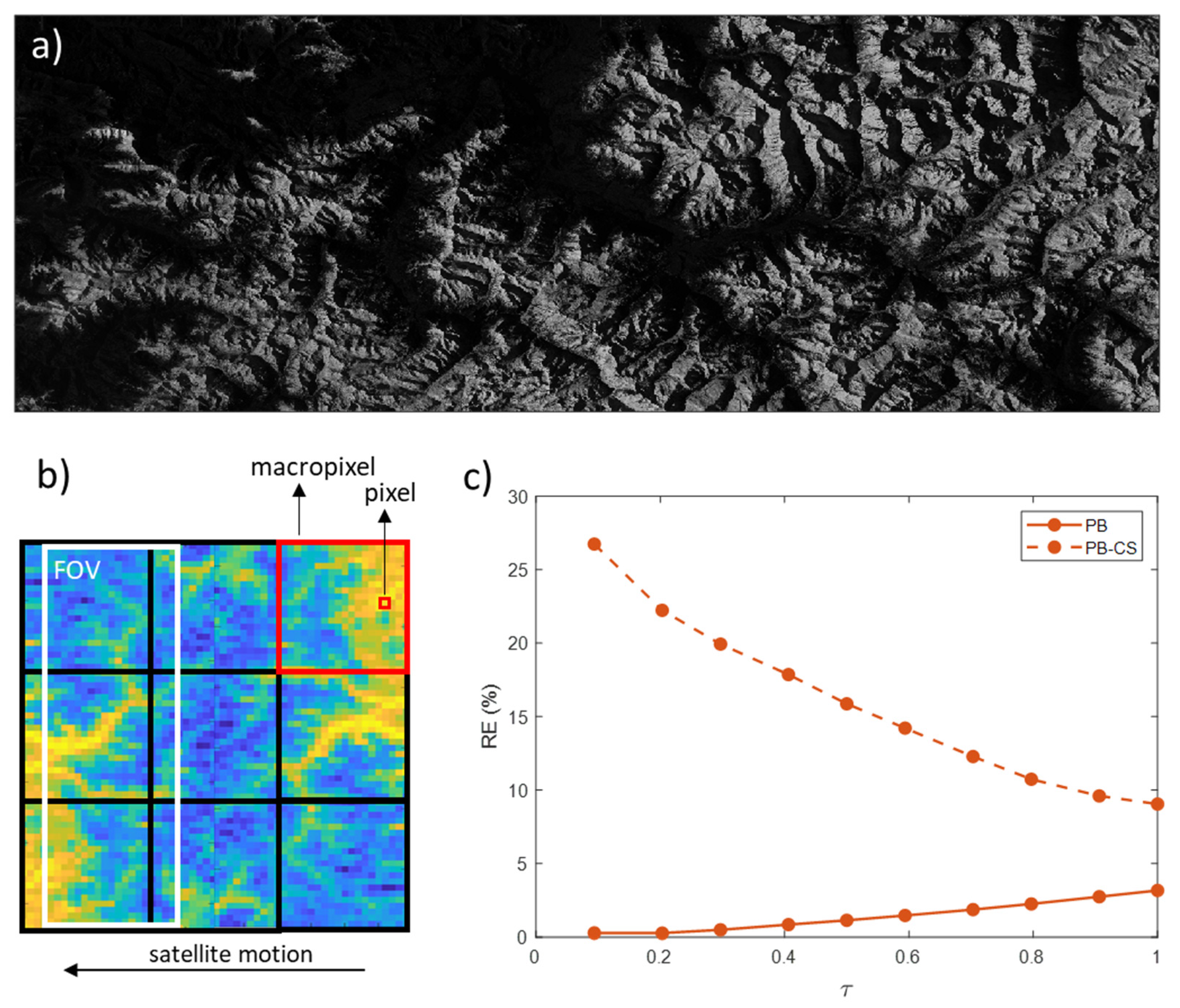
3.2. Reconstruction Performances of Dynamic Images

Up to now, we considered static images, as recorded, for example, by a geostationary satellite, or static images reconstructed line by line, to start mimicking the pushbroom acquisition. We will show hereafter the simulations performed to mimic the moving scene during the pushbroom CS (PB-CS) acquisition, in comparison with the classical pushbroom (PB) technique. In both cases, the field of view is linear, oriented across-track the satellite, and composed by $N\times 1$ sensing pixels.

In the pushbroom acquisition, we are dealing with a continuously moving scene. To simulate the movement, we apply a downsampling approach, working as follows. We consider as sensing pixel a macropixel, composed by $P$ pixels of the test image (Figure 5b). P is in the order of a few tens. The field of view is hence represented by a line of $N\times 1$ macropixels, or $NP\times P$ pixels. Since the scene is moving, it takes time equal to the dwell time for the field of view to move to the following macropixel. At any instant, the image is shifted one pixel along track to simulate the motion of the satellite, while the acquisition is integrated inside the macropixel. After a dwell time, we end up with a set of frames, which are processed depending on the acquisition strategy. In the case of the PB acquisition, we sum up all the frames and we integrate the intensity inside the macropixel. In the case of the PB-CS, we apply a 1D mask to each macropixel column, and we reconstruct the vertical line of macropixels applying the CC-TVAL algorithm. This process is repeated independently for each column of macropixels, until the whole image is reconstructed line by line, in analogy with the reconstruction procedure described in the previous section. The reference image is obtained integrating the intensity inside the macropixel at half the dwell time.

To evaluate the possibility of acquiring the signal in a period shorter than the dwell time, we introduce the parameter $\tau$, defined as the ratio between the acquisition time and the dwell time. In the case of PB-CS, we now consider that $\tau$ equals $\rho =M/N$, i.e., it takes the dwell time to acquire all the $N$ masks. This choice is mainly driven by the technological restrictions of such systems, usually limited by the modulator framerate. Figure 5a reports the image (in the G channel) used for the simulations, and Figure 5c the RE as a function of $\tau$, in both the PB and PB-CS acquisition methods. For this simulation we used $P=64, N=64, {\sigma }_{noise}=0$.

PB reaches better performances than PB-CS in every conditions and it is more accurate for smaller $\tau$ values. This is consistent with the fact that the scene is more stable when the acquisition time decreases. In practice, in PB acquisitions the exposure time is usually shorter than the dwell time in order to increase the along-track resolution, otherwise degraded by the image motion. On the contrary, the PB-CS method gets better results as $\tau$ increases; hence as the acquisition time approaches the dwell time, because the number of masks is larger and more details at higher spatial frequencies can be reconstructed. Clearly, since the scene is moving, the last masks are applied to a very different FOV with respect to the first ones, and the overall reconstruction accuracy is worse than in the PB method.

The spatial distribution of the reconstruction error as function of $\tau$ is reported in Figure 6, for both the PB and the PB-CS acquisition methods. We perform a Fourier analysis, which is useful to highlight the differences in the reconstruction accuracy both along track and across track, and we show the ratio between the 2D fast Fourier transformations (FFT) of the reconstructed images and the reference images, at different $\tau$ values. The PB always shows a higher reconstruction accuracy across track (y direction), while along track the errors increase with $\tau$, especially at high spatial frequencies. Considering that the parameter $\tau$ corresponds to the ratio between the acquisition time and the dwell-time, this confirms that the expected ground resolution along track is not ensured when the acquisition time approaches the dwell time. In the PB-CS case, the errors increase when the ratio $\tau$ decreases, i.e., when fewer masks are used for the reconstruction, for the lack of completeness in the bases set. Going from the highest to the lowest $\tau$, some horizontal lines (along track) appear in the Fourier images, meaning that we are losing information about specific spatial frequencies across track. Reducing the acquisition time by reducing the number of masks is not effective in reducing the reconstruction errors.

The important point to highlight is that, when the basis set is complete ($M=N$), we obtain the same spatial distribution of the errors for both the PB-CS and PB acquisition methods. Accordingly, following the evolution of the PB errors with the acquisition time, we can infer that, to reduce the reconstruction errors in the PB-CS case, we acquire all the masks in a time (much) shorter than the dwell time.

Taking into account the technological limitations of the focal plane modulators, this is possible only by splitting the acquisition process, spatially or temporally (or both), as reported in Figure 7a–c. The former approach is the so called block CS method [50,51], where the linear focal plane is spatially partitioned in blocks, each one detected by a single pixel detector. In this manner, the number of masks to be acquired in each block is $N/K$, where $K$ is the number of blocks, and the acquisition time is hence reduced by the same factor (Figure 7b). The latter approach is the pushframe method [38,52], and consists in partitioning the acquisition of the linear focal plane temporally, by exploiting the intrinsic motion of the scene. The pushframe camera can be viewed as a parallelized single pixel camera, where only $N/K$ masks are acquired by each pixel camera before the scene is passing away, as shown in Figure 7c.

The simulation results, without considering any registration or synchronization error, are shown in Figure 7d. The errors decrease with $K$, both in the visible and thermal bands, with approximately an inverse proportionality. Notably, the RE decreases to the values typical of the PB acquisition (a few percent) also in the visible region. We have to consider that, increasing the number of blocks, the complexity of the telescope focal plane increases, since each channel is acquired separately from the others. Nevertheless, this strategy gives a valid alternative to the traditional acquisition methods when detectors with a large number of pixels and a small pixel size are not available, or available at a prohibitive cost. All this analysis is valid when data with very low errors are required, or constraints on the acquisition time are present, in space applications; in all the other cases, the PB-CS acquisition method, performed as in Figure 7a, may be a valid alternative to the classical PB acquisition.

4. Conclusions

With the goal to evaluate the feasibility of a spatial multispectral pushbroom acquisition system for earth observation based on the spatial compressive sensing (CS) method, we conducted a series of analysis to address the performances of this method on images of the earth in the visible and thermal spectral domains. Given that the observations are devoted to the precise measurement of the earth radiance in the visible and thermal regions, we considered the reconstruction error as the benchmark. We reconstructed, in the different spectral bands, static images as a whole (framing acquisition), static images line by line, and dynamic images line by line, considering the image motion during acquisition (pushbroom acquisition).

The explored basis set (DCT, HD, CC) and reconstruction methods (TVAL, direct) do not strongly affect the reconstruction error in framing acquisitions, but they affect the computation time. On the contrary, in the pushframe acquisition strategy, the CC basis set is preferred for better performances when $M<N$, even if it is computationally more expensive. In this respect, when $M$ approaches $N$, the direct-CC is the best solution for the computation time reduction. In this case, in fact, the ordering of the CC basis and the almost completeness of the acquisition set produce reasonable approximations of the images.

In general, we observed an unexpected large variability of the reconstruction error within our homogenous set of representative images, both between the wavelength channels and within the same channel. This evidence may, in principle, be an issue for real systems, since the actual scene is not known before acquisition, and, accordingly, its maximum reconstruction error cannot be determined a priori. Notably, this problem may be overcome when $M=N$, i.e., when the acquisition set is complete and all the information is acquired.

Except this specific behavior with the image characteristics, an increase of the reconstruction error was observed moving from the static to the pushbroom acquisition methods, indicating that the movement affects the information acquisition. In particular, with a fixed number of acquired masks $M$, the RE increases as the total acquisition time increases, in a similar way as the classical PB acquisition, producing errors in the along track direction. Instead, with a fixed acquisition time, the RE increases when the number of masks is reduced, producing mainly across track errors at specific spatial frequencies. Reducing the acquisition time by reducing the number of masks is not effective in reducing the reconstruction errors.

With the idea of bringing a PB-CS system in operation, these simulations give advice on the acquisition parameters, which are mandatory to obtain high accuracy measurements, in a trade-off between the reconstruction error, the number of acquired masks, and the total acquisition time. The completeness of the acquisitions in a time (much) shorter than the dwell time is able to limit the reconstruction errors and to produce scientific level data. The splitting of the acquisition over multiple lines or in blocks is a valid solution to overcome the technological limitations of the present hardware, which, unfortunately, usually crash with other technical mission requirements. In fact, a good balancing between the FOV and the spatial resolution, which sets the total number of information, and the required framerate, which is limited by the modulator frame rate, is necessary for the successful design of such a PB-CS acquisition system.

In summary, we believe to have provided evidence on the goodness of this approach for future space missions, with particular attention to those that exploit both optical and thermal channels useful for cryosphere monitoring.

References

1. Elmasry, G.; Kamruzzaman, M.; Sun, D.W.; Allen, P. Principles and Applications of Hyperspectral Imaging in Quality Eval-uation of Agro-Food Products: A Review. Crit. Rev. Food Sci. Nutr. 2012, 52, 999–1023. [Google Scholar] [CrossRef] [PubMed]
2. Adão, T.; Hruška, J.; Pádua, L.; Bessa, J.; Peres, E.; Morais, R.; Sousa, J.J. Hyperspectral imaging: A review on UAV-based sensors, data processing and applications for agriculture and forestry. Remote Sens. 2017, 9, 1110. [Google Scholar] [CrossRef] [Green Version]
3. Jia, T.; Chen, D.; Wang, J.; Xu, D. Single-Pixel Color Imaging Method with a Compressive Sensing Measurement Matrix. Appl. Sci. 2018, 8, 1293. [Google Scholar] [CrossRef] [Green Version]
4. Boldrini, B.; Kessler, W.; Rebner, K.; Kessler, R.W. Hyperspectral Imaging: A Review of Best Practice, Performance and Pitfalls for in-line and on-line Applications. J. Near Infrared Spectrosc. 2012, 20, 483–508. [Google Scholar] [CrossRef]
5. Lu, G.; Fei, B. Medical hyperspectral imaging: A review. J. Biomed. Opt. 2014, 19, 010901. [Google Scholar] [CrossRef]
6. Dong, X.; Jakobi, M.; Wang, S.; Köhler, M.H.; Zhang, X.; Koch, A.W. A review of hyperspectral imaging for nanoscale materials research. Appl. Spectrosc. Rev. 2018, 54, 285–305. [Google Scholar] [CrossRef]
7. Manolakis, D.; Lockwood, R.; Cooley, T. Hyperspectral Imaging Remote Sensing: Physics, Sensors, and Algorithms; Cambridge University Press: Cambridge, UK, 2016; pp. 1–709. ISBN 9781107083660. [Google Scholar]
8. Sandau, R. Status and trends of small satellite missions for Earth observation. Acta Astronaut. 2010, 66, 1–12. [Google Scholar] [CrossRef]
9. Staenz, K.; Mueller, A.; Heiden, U. Overview of terrestrial imaging spectroscopy missions. In Proceedings of the 2013 IEEE International Geoscience and Remote Sensing Symposium—IGARSS, Melbourne, Australia, 21–26 July 2013; pp. 3502–3505. [Google Scholar]
10. Belward, A.S.; Skøien, J.O. Who launched what, when and why; trends in global land-cover observation capacity from civilian earth observation satellites. ISPRS J. Photogramm. Remote Sens. 2015, 103, 115–128. [Google Scholar] [CrossRef]
11. National Research Council. National Research Council Earth Science and Applications from Space: National Imperatives for the Next Decade and Beyond; The National Academies Press: Washington, DC, USA, 2007; pp. 1–428. [Google Scholar]
12. Paganini, M.; Petiteville, I.; Ward, S.; Dyke, G.; Steventon, M.; Harry, J.; Kerblat, F. Satellite Earth Observations in Support of the Sustainable Development Goals: The CEOS Earth Observation Handbook; Special 2018 Edition; The Committee on Earth Observation Satellites and the European Space Agency: Paris, France, 2018. [Google Scholar]
13. Chuvieco, E. Earth Observation of Global Change; Springer: New York, NY, USA, 2008; ISBN 9781402063572. [Google Scholar]
14. Cogliati, S.; Sarti, F.; Chiarantini, L.; Cosi, M.; Lorusso, R.; Lopinto, E.; Miglietta, F.; Genesio, L.; Guanter, L.; Damm, A.; et al. The PRISMA imaging spectroscopy mission: Overview and first performance analysis. Remote Sens. Environ. 2021, 262, 112499. [Google Scholar] [CrossRef]
15. Candès, E.; Romberg, J. L1 Magic: Recovery of Sparse Signals via Convex Programming; California Institute of Technology: Pasadena, CA, USA, 2005; Available online: http://brainimaging.waisman.wisc.edu/~chung/BIA/download/matlab.v1/l1magic-1.1/l1magic_notes.pdf (accessed on 28 December 2021).
16. Candès, E.J.; Romberg, J.K.; Tao, T. Stable signal recovery from incomplete and inaccurate measurements. Commun. Pure Appl. Math. 2006, 59, 1207–1223. [Google Scholar] [CrossRef] [Green Version]
17. Candes, E.J.; Wakin, M. An Introduction to Compressive Sampling. IEEE Signal Process. Mag. 2008, 25, 21–30. [Google Scholar] [CrossRef]
18. Donoho, D.L. Compressed sensing. IEEE Trans. Inf. Theory 2006, 52, 1289–1306. [Google Scholar] [CrossRef]
19. Duarte, M.; Sarvotham, S.; Baron, D.; Wakin, M.; Baraniuk, R. Distributed Compressed Sensing of Jointly Sparse Signals. In Proceedings of the Conference Record of the Thirty-Ninth Asilomar Conference on Signals, Systems and Computers, Pacific Grove, CA, USA, 30 October–2 November 2005; pp. 1537–1541. [Google Scholar] [CrossRef] [Green Version]
20. Haupt, J.; Nowak, R. Signal Reconstruction from Noisy Random Projections. IEEE Trans. Inf. Theory 2006, 52, 4036–4048. [Google Scholar] [CrossRef]
21. Baraniuk, R.G. Compressive Sensing. IEEE Signal Process. Mag. 2007, 24, 118–124. [Google Scholar] [CrossRef]
22. Duarte, M.F.; Davenport, M.A.; Takbar, D.; Laska, J.N.; Sun, T.; Kelly, K.F.; Baraniuk, R.G. Single-pixel imaging via compres-sive sampling: Building simpler, smaller, and less-expensive digital cameras. IEEE Signal Process. Mag. 2008, 25, 83–91. [Google Scholar] [CrossRef] [Green Version]
23. Takhar, D.; Laska, J.N.; Wakin, M.; Duarte, M.; Baron, D.; Sarvotham, S.; Kelly, K.; Baraniuk, R.G. A new compressive imaging camera architecture using optical-domain compression. In Proceedings of the Computational Imaging IV, San Jose, CA, USA, 15 January 2006; Volume 6065, p. 606509. [Google Scholar]
24. Gibson, G.M.; Johnson, S.D.; Padgett, M.J. Single-pixel imaging 12 years on: A review. Opt. Express 2020, 28, 28190. [Google Scholar] [CrossRef] [PubMed]
25. Sun, T.; Kelly, K. Compressive Sensing Hyperspectral Imager. In Proceedings of the Frontiers in Optics 2009/Laser Science XXV/Fall 2009 OSA Optics & Photonics Technical Digest, San Jose, CA, USA, 11–15 October 2009; p. CTuA5. [Google Scholar]
26. Chen, H.; Asif, S.; Sankaranarayanan, A.; Veeraraghavan, A. FPA-CS: Focal plane array-based compressive imaging in short-wave infrared. In Proceedings of the 2015 IEEE Conference on Computer Vision and Pattern Recognition (CVPR), Boston, MA, USA, 7–12 June 2015; pp. 2358–2366. [Google Scholar]
27. Mahalanobis, A.; Shilling, R.; Murphy, R.; Muise, R. Recent results of infrared compressive sensing. Appl. Opt. 2014, 53, 8060–8070. [Google Scholar] [CrossRef]
28. Gehm, M.; John, R.; Brady, D.J.; Willett, R.M.; Schulz, T.J. Single-shot compressive spectral imaging with a dual-disperser architecture. Opt. Express 2007, 15, 14013–14027. [Google Scholar] [CrossRef]
29. Wagadarikar, A.; John, R.; Willett, R.; Brady, D. Single disperser design for coded aperture snapshot spectral imaging. Appl. Opt. 2008, 47, B44–B51. [Google Scholar] [CrossRef] [Green Version]
30. Arce, G.R.; Brady, D.J.; Carin, L.; Arguello, H.; Kittle, D.S. Compressive Coded Aperture Spectral Imaging: An Introduction. IEEE Signal Process. Mag. 2014, 31, 105–115. [Google Scholar] [CrossRef]
31. Wu, Y.; Mirza, O.; Arce, G.R.; Prather, D.W. Development of a digital-micromirror-device-based multishot snapshot spectral imaging system. Opt. Lett. 2011, 36, 2692–2694. [Google Scholar] [CrossRef] [PubMed] [Green Version]
32. August, Y.; Vachman, C.; Rivenson, Y.; Stern, A. Compressive hyperspectral imaging by random separable projections in both the spatial and the spectral domains. Appl. Opt. 2013, 52, D46–D54. [Google Scholar] [CrossRef]
33. Baraniuk, R.G.; Goldstein, T.; Sankaranarayanan, A.; Studer, C.; Veeraraghavan, A.; Wakin, M. Compressive Video Sensing: Algorithms, architectures, and applications. IEEE Signal Process. Mag. 2017, 34, 52–66. [Google Scholar] [CrossRef]
34. Edgar, M.P.; Gibson, G.; Bowman, R.; Sun, B.; Radwell, N.; Mitchell, K.J.; Welsh, S.; Padgett, M. Simultaneous real-time visible and infrared video with single-pixel detectors. Sci. Rep. 2015, 5, 10669. [Google Scholar] [CrossRef] [PubMed]
35. Fowler, J.E. Compressive pushbroom and whiskbroom sensing for hyperspectral remote-sensing imaging. In Proceedings of the 2014 IEEE International Conference on Image Processing (ICIP), Paris, France, 27–30 October 2014; pp. 684–688. [Google Scholar]
36. Pariani, G.; Zanutta, A.; Basso, S.; Bianco, A.; Striano, V.; Sanguinetti, S.; Colombo, R.; Genoni, M.; Benetti, M.; Freddi, R.; et al. Compressive sampling for multispectral imaging in the vis-NIR-TIR: Optical design of space telescopes. In Proceedings of the Space Telescopes and Instrumentation 2018: Optical, Infrared, and Millimeter Wave, Austin, TX, USA, 10–15 June 2018; Volume 10698, p. 106985O. [Google Scholar]
37. Guzzi, D.; Coluccia, G.; Labate, D.; Lastri, C.; Magli, E.; Nardino, V.; Palombi, L.; Pippi, I.; Coltuc, D.; Marchi, A.Z.; et al. Optical compressive sensing technologies for space applications: Instrumental concepts and performance analysis. In Proceedings of the International Conference on Space Optics—ICSO 2018, Chania, Greece, 12 July 2019; Volume 11180, p. 111806B. [Google Scholar]
38. Noblet, Y.; Bennett, S.; Griffin, P.F.; Murray, P.; Marshall, S.; Roga, W.; Jeffers, J.; Oi, D. Compact multispectral pushframe camera for nanosatellites. Appl. Opt. 2020, 59, 8511. [Google Scholar] [CrossRef]
39. Arnob, M.P.; Nguyen, H.; Han, Z.; Shih, W.-C. Compressed sensing hyperspectral imaging in the 09–25 μm shortwave infrared wavelength range using a digital micromirror device and InGaAs linear array detector. Appl. Opt. 2018, 57, 5019–5024. [Google Scholar] [CrossRef]
40. Willett, R.; Duarte, M.F.; Davenport, M.A.; Baraniuk, R.G. Sparsity and Structure in Hyperspectral Imaging: Sensing, Reconstruction, and Target Detection. IEEE Signal Process. Mag. 2013, 31, 116–126. [Google Scholar] [CrossRef] [Green Version]
41. Colombo, R.; Garzonio, R.; Di Mauro, B.; Dumont, M.; Tuzet, F.; Cogliati, S.; Pozzi, G.; Maltese, A.; Cremonese, E. Introducing Thermal Inertia for Monitoring Snowmelt Processes with Remote Sensing. Geophys. Res. Lett. 2019, 46, 4308–4319. [Google Scholar] [CrossRef]
42. Li, C. An Efficient Algorithm for Total Variation Regularization with Applications to the Single Pixel Camera and Compressive Sensing. Master’s Thesis, Rice University, Houston, TX, USA, September 2009. [Google Scholar]
43. Candes, E.J.; Romberg, J.; Tao, T. Robust uncertainty principles: Exact signal reconstruction from highly incomplete frequency information. IEEE Trans. Inf. Theory 2006, 52, 489–509. [Google Scholar] [CrossRef] [Green Version]
44. Bai, H.; Wang, A.; Zhang, M. Compressive Sensing for DCT Image. In Proceedings of the 2010 International Conference on Computational Aspects of Social Networks, Taiyuan, China, 26–28 September 2010; pp. 378–381. [Google Scholar]
45. Zhou, G.; Du, Y. A MEMS-driven Hadamard transform spectrometer. In Proceedings of the MOEMS and Miniaturized Systems XVII, San Francisco, CA, USA, 30–31 January 2018; Volume 10545, p. 105450X. [Google Scholar]
46. Yu, W.-K. Super Sub-Nyquist Single-Pixel Imaging by Means of Cake-Cutting Hadamard Basis Sort. Sensors 2019, 19, 4122. [Google Scholar] [CrossRef] [Green Version]
47. Sun, M.-J.; Meng, L.-T.; Edgar, M.P.; Padgett, M.J.; Radwell, N. A Russian Dolls ordering of the Hadamard basis for compressive single-pixel imaging. Sci. Rep. 2017, 7, 3464. [Google Scholar] [CrossRef] [PubMed] [Green Version]
48. Irons, J.R.; Dwyer, J.L. An overview of the Landsat Data Continuity Mission. In Proceedings of the SPIE Defense, Security, and Sensing, Orlando, FL, USA, 29 April 2010; Volume 7695, p. 769508. [Google Scholar]
49. Knight, E.J.; Kvaran, G. Landsat-8 Operational Land Imager Design, Characterization and Performance. Remote Sens. 2014, 6, 10286–10305. [Google Scholar] [CrossRef] [Green Version]
50. Gan, L. Block Compressed Sensing of Natural Images. In Proceedings of the 2007 15th International Conference on Digital Signal Processing, Cardiff, UK, 1–4 July 2007; pp. 403–406. [Google Scholar]
51. Ke, J.; Lam, E.Y. Object reconstruction in block-based compressive imaging. Opt. Express 2012, 20, 22102–22117. [Google Scholar] [CrossRef] [PubMed]
52. Bennett, S.; Noblet, Y.; Griffin, P.F.; Murray, P.; Marshall, S.; Jeffers, J.; Oi, D. Compressive Sampling Using a Pushframe Camera. IEEE Trans. Comput. Imaging 2021, 7, 1069–1079. [Google Scholar] [CrossRef]
Figure 1. Example of four (AD) Landsat 8 images in the blue channel acquired on the 16 January 2020 on the Italian Alps.
Remotesensing 14 00333 g001
Figure 2. Reconstruction error of the representative image (box A, Figure 1) in the different wavelength bands as function of the selected bases and M / N ratio. σ n o i s e = 5 % in all boxes.
Remotesensing 14 00333 g002
Figure 3. Reconstruction errors of a representative image (box A, Figure 1) in three wavelength bands as function of the reconstruction method and M / N ratio. σ n o i s e = 0 % (top) and σ n o i s e = 5 % (bottom).
Remotesensing 14 00333 g003
Figure 4. Four representative images of the Alps in the G and TIR channels, the normalized intensity of the vector s in the two channels, and the reconstruction error in all channels as function of the factor M / N . Image (A) represents mountains covered by snow, (B,C) mountains without snow, and (D) a portion of scene covered by clouds. For each image, we performed the simulated acquisition and reconstruction with the CC-direct method and σ n o i s e = 0 .
Remotesensing 14 00333 g004
Figure 5. Image in the G channel used in the simulations (a). Schematic of the simulations in case of a moving scene (b). Reconstruction error in the G channel as function of the ratio between acquisition time and dwell time (c).
Remotesensing 14 00333 g005
Figure 6. Fourier analysis of the PB (left) and PB-CS (right) acquisition methods for different τ values. Images are the logarithm of the ratio between the 2D fast Fourier transformations (FFT) of the reconstructed image and the reference image. x   is the direction of movement.
Remotesensing 14 00333 g006
Figure 7. PB-CS acquisition concepts: (a) N masks are acquired during the dwell time; (b) block CS, where the linear focal plane is spatially divided in K pixels; (c) multi-linear focal plane, or pushframe, where the whole set of masks are acquired in K subsequent steps, when the scene passes by; the arrow indicates the direction of motion. (d) Reconstruction error in the G and TIR bands as function of the number of blocks. Points at K = 1 represent case (a), the other points either cases (b) or (c).
Remotesensing 14 00333 g007