Multi-Layer Overlapped Subaperture Algorithm for Extremely-High-Squint High-Resolution Wide-Swath SAR Imaging with Continuously Time-Varying Radar Parameters

Abstract

Extremely-high-squint (EHS) geometry of the traditional constant-parameter synthetic aperture radar (SAR) induces non-orthogonal wavenumber spectrum and hence the distortion of point spread function (PSF) in focused images. The method invented to overcome this problem is referred to as new-concept parameter-adjusting SAR. It corrects the PSF distortion by adjusting radar parameters, such as carrier frequency and chirp rate, based on instant data acquisition geometry. In this case, the characteristic of signal is quite different from the constant-parameter SAR and therefore, the traditional imaging algorithms cannot be directly applied for parameter-adjusting SAR imaging. However, the existing imaging algorithm for EHS parameter-adjusting SAR suffers from insufficient accuracy if a high-resolution wide-swath (HRWS) performance is required. Thus, this paper proposes a multi-layer overlapped subaperture algorithm (ML-OSA) for EHS HRWS parameter-adjusting SAR imaging with three main contributions: First, a more accurate signal model with time-varying radar parameters in high-squint geometry is derived. Second, phase errors are compensated with much higher accuracy by implementing multiple layers of coarse-to-fine spatially variant filters. Third, the analytical swath limit of the ML-OSA is derived by considering both the residual errors of signal model and phase compensations. The presented approach is validated via both the point- and extended-target computer simulations.

1. Introduction

Extremely-high-squint (EHS) synthetic aperture radar (SAR) is of significance due to its applicability in multi-aspect observation, missile guidance, etc. [1,2,3,4,5,6]. Comparing to the ordinary broadside geometry, EHS SAR has a more seriously coupled echoes and hence imposes two main challenges for imaging. First, a high-squint geometry is to form non-orthogonal range and azimuth directions and hence non-orthogonal wavenumber spectrum. Such a spectrum is to cause distorted point spread function (PSF) of target, which means resolution performance degradation in a focused image [7,8,9,10,11]. Second, the serious coupling between range and azimuth is often characterized by spatial variance and hence is hard to remove via efficient frequency domain algorithms [12,13,14].

The first challenge can be overcome by using a parameter-adjusting SAR for waveform spectrum correction and hence PSF distortion correction [15,16,17]. The basic mechanism is that while the format of waveform spectrum is jointly determined by data acquisition geometry and radar parameters, the radar parameters, like carrier frequency and chirp rate, can be adjusted pulse-by-pulse according to instant data acquisition geometry to counteract the negative influence of EHS geometry on waveform spectrum format. Thus, an expected orthogonal wavenumber spectrum and hence optimum PSF of target can be achieved.

There exists plenty of studies trying to solve the second challenges in the traditional constant-parameter SAR. For example, modified range-Doppler algorithm [18,19,20], extended nonlinear chirp scaling algorithm [21,22,23,24,25,26,27,28,29] and extended range migration algorithm [30,31,32,33] have been proposed for the high-squint constant-parameter mode. However, the accuracy of range-Doppler domain algorithms is insufficient in the EHS HRWS SAR due to inaccurate range-Doppler spectrum expression. More importantly, the constant-parameter SAR is very premise for most of existing SAR imaging algorithms. They cannot be directly applied for EHS parameter-adjusting SAR imaging due to different characteristic of signal with time-varying radar parameters.

According to the strategy of adjusting radar parameters for wavenumber spectrum correction in parameter-adjusting SAR, wavenumber domain algorithms, such as the polar format algorithm (PFA) [15] and overlapped subaperture algorithm (OSA) [16], have shown the advantages in imaging EHS parameter-adjusting SAR echoes. The accuracy of these wavenumber domain algorithm is directly determined by the residual phase error after compensating the phase errors led by the necessary planar wavefront assumption (PWA). In the case of requiring high-resolution wide-swath (HRWS) performance in an EHS geometry, the existing wavenumber domain imaging algorithms for parameter-adjusting SAR will fail due to insufficient accuracy caused by less accurate signal model and less accurate phase compensation processing [15,16].

In this paper, a multi-layer overlapped subaperture algorithm (ML-OSA) is proposed for EHS HRWS parameter-adjusting SAR imaging. ML-OSA focuses on the new-concept parameter-adjusting SAR imaging rather than the traditional constant-parameter SAR imaging. Comparing to the existing imaging algorithms for parameter-adjusting SAR, the new one is also a wavenumber domain algorithm but outperforms in three main aspects:

• A more accurate signal model with time-varying parameters is employed. Comparing to the existing ones, the new signal model includes the complete expansion of two-dimensional Taylor series and hence is able to describe the residual PWA phase errors with a much improved accuracy.
• A more precise phase error compensation method is proposed via multi-level coarse-to-fine focusing. Coarsely focused images are used as references for compensator generation to remove spatially variant PWA phase errors. The new processing describes the coarse image distortion caused by the linear components of the PWA phase error with a much improved accuracy and hence contributes to much less residual phase error.
• The accuracy of the proposed ML-OSA is analytically presented in the form of swath limit in a certain resolution level. The algorithm accuracy analysis is more accurate than the existing ones by considering the effects of both the precision of signal model and multi-level phase compensation.

This paper is organized as follows. Section 2 briefly reviews the mechanism and necessity of the parameter-adjusting SAR. Section 3 derives the proposed ML-OSA for EHS HRSW SAR imaging. Section 4 analyzes the accuracy of the proposed algorithm in the form of swath limit. Section 5 discusses the non-ideal factors from the non-ideal trajectory and the precise of parameter adjustment. The presented approach is evaluated in Section 6 by the computer simulations. Section 7 summarizes this study and suggests future researches.

2. Overview of Parameter-Adjusting SAR

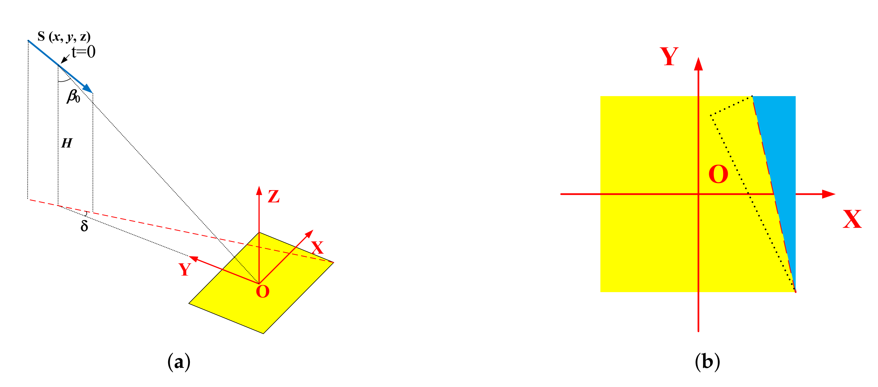
2.1. Geometry and Signal Model

Take the geometry of EHS SAR in Figure 1 as an example. The origin O of the coordinate system locates at the scene center, and the Y-axis is collinear with the projection of the slant range onto XOY plane (ground plane) at the central synthetic aperture time. In order to simplify the analysis, the sensor is assumed to move linearly with the dive angle $\varphi$ and the complementary angle of ground squint angle $\delta$. The coordinate of an arbitrary sample position of the sensor along the flight path are assumed to be $(x,y,z)$. Point A represents the position of the sensor at central synthetic aperture time with coordinate $(0,Y_{\mathrm{c}},H)$. Furthermore, $\beta$ is the instantaneous incidence angle, the $R_{\mathrm{c}}$ denotes the instant distance from the sensor to the scene center and the $R_{\mathrm{p}}$ represents the instantaneous distance from the sensor to an arbitrary scatterer P with the coordinate $(x_{\mathrm{p}},y_{\mathrm{p}},0)$. $\alpha$ is the angle between the projection of $OS$ on the XOY and Y-axis.

In the case of transmitting a linear frequency modulation (LFM) signal, the backscattered echo of target P yields

$$\begin{array}{cc}\hfill S_0(\tau ,t)& =\mathrm{rect}\left[{\displaystyle \frac{\tau -2R_{\mathrm{p}}\left(t\right)/c}{T_{\mathrm{p}}}}\right]\mathrm{rect}\left[{\displaystyle \frac{t-t_{\mathrm{c}}}{T_{\mathrm{syn}}}}\right]exp\left\{j\pi \gamma {\left(\tau -\frac{2R_{\mathrm{p}}\left(t\right)}{c}\right)}^2\right\}\hfill \\ \hfill & ·exp\left\{-j{\displaystyle \frac{4\pi f_{\mathrm{c}}{R}_{\mathrm{p}}\left(t\right)}{c}}\right\}exp\left\{j2\pi f_{\mathrm{c}}t\right\}\hfill \end{array}$$

(1)

where c is the light speed, $\tau$ and t are the fast and the slow time, $T_{\mathrm{p}}$ represents the pulse width, $t_{\mathrm{c}}$ and $T_{\mathrm{syn}}$ are the central synthetic aperture time and the synthetic aperture time, respectively, $f_{\mathrm{c}}$ denotes the carrier frequency, $\gamma$ is the chirp rate, and rect[·] depicts the rectangular function. After the operations of two-dimensional dechirping and residual video phase (RVP) removal, the backscattered signal can be digitally recorded as

$$\begin{array}{cc}\hfill S_1(i,m)& =exp\left\{j{\displaystyle \frac{4\pi }{c}}\left(f_{\mathrm{c}}+{\displaystyle \frac{\gamma }{F_{\mathrm{s}}}}i\right)\left(R_{\mathrm{c}}\left(m\right)-R_{\mathrm{p}}\left(m\right)\right)\right\}=exp\left\{j{K}_{\mathrm{R}}\left(i\right)R_{\Delta }\left(m\right)\right\}\hfill \\ \hfill & \left(i=-{\displaystyle \frac{N_{\mathrm{r}}}{2}},\cdots {\displaystyle \frac{N_{\mathrm{r}}}{2}},m=-{\displaystyle \frac{N_{\mathrm{a}}}{2}},\cdots {\displaystyle \frac{N_{\mathrm{a}}}{2}}\right)\hfill \end{array}$$

(2)

where $N_{\mathrm{r}}$ and $N_{\mathrm{a}}$ indicate the sample point number in the range and azimuth dimension, respectively. i and m are the the sampling indexes of range and azimuth, respectively. Furthermore, $F_{\mathrm{s}}$ represents the sampling rate. The radial wavenumber $K_{\mathrm{R}}$ is defined as $4\pi \left(f_{\mathrm{c}}+\gamma /F_{\mathrm{s}}i\right)/c$. The azimuth wavenumber $K_{\mathrm{x}}$ and the range wavenumber $K_{\mathrm{y}}$ are obtained by projecting $K_{\mathrm{R}}$ to the X-axis and Y-axis respectively. If the PWA phase error is temporarily ignored [34,35,36], (2) can be further expressed as

$$S_2(i,m)=exp\left\{j\left(K_{\mathrm{x}}\left(i,m\right)x_{\mathrm{p}}+K_{\mathrm{y}}\left(i,m\right)y_{\mathrm{p}}\right)\right\}$$

(3)

where

$$K_{\mathrm{x}}(i,m)={\displaystyle \frac{4\pi }{c}}\left(f_{\mathrm{c}}+{\displaystyle \frac{\gamma }{F_{\mathrm{s}}}}i\right)sin\beta \left(m\right)sin\alpha \left(m\right),K_{\mathrm{y}}(i,m)={\displaystyle \frac{4\pi }{c}}\left(f_{\mathrm{c}}+{\displaystyle \frac{\gamma }{F_{\mathrm{s}}}}i\right)sin\beta \left(m\right)cos\alpha \left(m\right)$$

(4)

2.2. Limit of Constant-Parameter SAR with EHS Geometry

In the constant-parameter case, the wavenumber spectrum and PSF are severely distorted as shown in Figure 2, due to the EHS SAR geometry. The PSF distortion results in non-uniform spatial resolution. In addition, the directions of range and azimuth are no longer orthogonal and the resolutions of range and azimuth are not the maximum or minimum value of the resolutions along all directions [9,10,11]. In the EHS SAR, the severely skewed wavenumber spectrum is drawn in Figure 2a, with the coordinates defined by $K_{\mathrm{x}}$ and $K_{\mathrm{y}}$. In Figure 2a, the grey area in the middle of the wavenumber spectrum is the valid data of backscattered signal. Furthermore, point C represents the sampling point with coordinate $(K_{\mathrm{x}}(0,0),K_{\mathrm{y}}(0,0))$. And the dotted red curve is the azimuth sampling points with coordinates $(K_{\mathrm{x}}(0,m),K_{\mathrm{y}}(0,m))$. In order to analyze the inclination of the wavenumber spectrum, the solid red line L denotes the tangent of the dotted red curve at point C. The slope of the tangent line L is represented by k which is also the tangent value of the distorted angle ${\Psi }_{\mathrm{k}}$. Thus, it is necessary to derive the expression of k.

According to (A6) in Appendix A, ${\Psi }_{\mathrm{k}}$ can be denoted as

$${\Psi }_{\mathrm{k}}=arctan\left(-{\displaystyle \frac{{cos}^2{\beta }_{0}cos\varphi cos\delta -sin{\beta }_{0}cos{\beta }_{0}sin\varphi }{cos\varphi sin\delta }}\right)$$

(5)

The distorted PSF with constant radar parameters is plotted in Figure 2b. The horizontal red line and the oblique red line are the azimuth ground resolution ${\rho }_{\mathrm{ga}}$ and the range ground resolution ${\rho }_{\mathrm{gr}}$ respectively, and their included angle is defined as ${\Psi }_{\mathrm{r}}$. By deriving the projection coefficients between slant range plane and ground plane, the expression of ${\Psi }_{\mathrm{r}}$ is presented in [10] as

$${\Psi }_{\mathrm{r}}=arctan\left(-{\displaystyle \frac{cos\varphi sin\delta }{{cos}^2{\beta }_{0}cos\varphi cos\delta -sin{\beta }_{0}cos{\beta }_{0}sin\varphi }}\right)$$

(6)

By observing (5) and (6), it is obvious to conclude that ${\Psi }_{\mathrm{k}}$ and ${\Psi }_{\mathrm{r}}$ are complementary. Consequently, the distortion of wavenumber spectrum causes the PSF distortion. If the distorted spectrum can be corrected to the orthogonal spectrum, the PSF distortion can be removed and hence the imaging performance is improved.

2.3. Parameter-Adjusting SAR

Parameter-adjusting is a method proposed to correct the distorted wavenumber spectrum. The basic mechanism is that while the format of waveform spectrum is jointly determined by data acquisition geometry and radar parameters, the radar parameters, like carrier frequency and chirp rate, can be adjusted pulse-by-pulse according to instant data acquisition geometry to counteract the negative influence of EHS geometry on waveform spectrum format. In the constant-parameter case, $K_{\mathrm{y}}$ is affected by $\beta \left(m\right)$ and $\alpha \left(m\right)$, which are related to the sensor positions. To eliminate the distorted angle ${\Psi }_{\mathrm{k}}$ in Figure 2b, in other words, to obtain the tangent with slope $k=0$, $K_{\mathrm{y}}$ should remain unchanged during the synthetic aperture time. Thus, the radar parameters in (4) need to be redesigned to counteract the variety of $K_{\mathrm{y}}$. The parameter-adjusting strategy can be regulated as (7).

$$f_{\mathrm{c}}\left(m\right)=f_{\mathrm{c}0}{\displaystyle \frac{sin{\beta }_0}{sin\beta \left(m\right)cos\alpha \left(m\right)}}\gamma \left(m\right)={\gamma }_0{\displaystyle \frac{sin{\beta }_0}{sin\beta \left(m\right)cos\alpha \left(m\right)}}$$

(7)

where the parameters $f_{\mathrm{c}0}$ and ${\gamma }_0$ remain unchanged along the synthetic aperture time, are defined as the referential parameters. But the parameters $f_{\mathrm{c}}\left(m\right)$ and $\gamma \left(m\right)$ vary with radar positions, are defined as adjusted parameters. Then, by replacing $f_{\mathrm{c}}$ and $\gamma$ expressed in (4) with $f_{\mathrm{c}}\left(m\right)$ and $\gamma \left(m\right)$ expressed in (7) respectively, the wavenumber $K_{\mathrm{x}}$ and $K_{\mathrm{y}}$ can be rewritten as

$$K_{\mathrm{x}}(i,m)={\displaystyle \frac{4\pi }{c}}\left(f_{\mathrm{c}0}+{\displaystyle \frac{{\gamma }_0}{F_s}}i\right)sin{\beta }_{0}tan\alpha \left(m\right)K_{\mathrm{y}}\left(i\right)={\displaystyle \frac{4\pi }{c}}\left(f_{\mathrm{c}0}+{\displaystyle \frac{{\gamma }_0}{F_s}}i\right)sin{\beta }_0$$

(8)

Equation (8) indicates that $K_{\mathrm{y}}$ remains unchanged for each azimuth sample position. By employing this strategy in data acquisition, the orthogonal wavenumber spectrum is obtained as illustrated in Figure 3a. It can be seen that ${\Psi }_{\mathrm{k}}=0^{\circ }$. According to the derivation in the previous section, the angle ${\Psi }_{\mathrm{r}}$ drawn in Figure 3b is ${90}^{\circ }$, and the range resolution and azimuth resolution are orthogonal.

The comparison diagram of the −3 dB resolution ellipses of the constant-parameter and parameter-adjusting modes is described in Figure 4. The red ellipse and dashed lines indicate the resolution ellipse, azimuth and range resolutions in the EHS constant-parameter SAR, respectively, while the green ones represent the results in the EHS parameter-adjusting SAR. The resolution ellipse of constant-parameter SAR is distorted, but the vertical distance from the top edge to the bottom edge of ellipse is unchanged due to the unaltered bandwidth. Compared with constant-parameter case, the range resolution and the worst resolution of parameter-adjusting case have been significantly improved. In addition, the maximum resolution deterioration ratio $({\rho }_2-{\rho }_1)/{\rho }_1$ is higher than the maximum resolution optimization ratio $({\rho }_1-{\rho }_3)/{\rho }_1$. Therefore, this parameter-adjusting method enhances the spatial resolution of SAR imaging.

In order to prove the advantage of the time-varying parameter method, backprojection algorithm (BPA) with continuously time-varying carrier frequency and chirp rate is compared with BPA with constant-parameter method by simulating the scene center firstly. The simulation parameters are intuitively listed in the

Table 1. Key Simulation Parameters.

Parameter	Value	Parameter	Value
Carrier frequency	30.11∼29.83 GHz	Bandwidth	540 MHz
Pulse width	10 $\mathsf{\mu }$s	Chirp rate	54.23∼53.74 THz/s
Sensor velocity	1000 m/s	Sensor acceleration	100 m/s${}^2$
Pulse repeat frequency	7540 Hz	Central altitude	2 km
Central slant range	5.2 km	Central incidence angle	67.3${}^{\circ }$
Dive angle	30${}^{\circ }$	Squint angle	80.9${}^{\circ }$
Resolution	0.3 m × 0.3 m	Scene size	1200 m × 1200 m

. The squint angle in the simulation refers to the angle between the beam pointing and vertical-to-trajectory direction in the slant range plane. In Figure 5a,b, the variation range of carrier frequency $f_{\mathrm{c}}\left(m\right)$ and chirp rate $\gamma \left(m\right)$ are illustrated, respectively. The carrier frequency varies from 30.11 GHz to 29.83 GHz and the chirp rate ranges from 54.23 THz/s to 53.74 THz/s.

As is shown in Figure 5c, the PSF contour with constant parameter BPA is non-orthogonal. The angle between the azimuth and the range direction is 61${}^{\circ }$ calculated by (6). In contrast to constant-parameter method, our proposed solution is orthogonal displayed in Figure 5d. In addition, the worst resolution of BPA with constant parameter is about 0.43 m, yet the worst resolution of parameter-adjusting method is about 0.32 m. Therefore, the worst resolution is increased by approximately 26%. The maximum resolution deterioration ratio is 35% and the maximum resolution optimization ratio is 21% as expected.

The simulation of two close targets are conducted to verify the effectiveness of the proposed method in improving resolution ability. According to the previous simulation, (0, 0) and (0.12, −0.24) are placed on the ground plane, which are illustrated in Figure 6a. The focused SAR images of two point-targets with two methods are shown in Figure 6b and Figure 6c, respectively. It shows that the constant-parameter method cannot discriminate two targets clearly but the parameter-adjusting method can discriminate them.

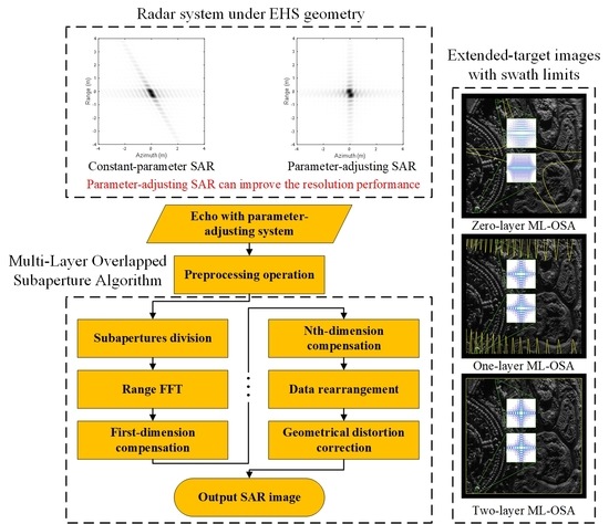
3. Multi-Layer Overlapped Subaperture Algorithm

3.1. Analysis of the PWA Phase Error

In the PFA, the linear and quadratic phase errors caused by the PWA result in the geometrical distortion and defocusing, respectively [36,37,38,39]. Therefore, an accurate phase model is required to compensate the PWA phase error for the EHS HRWS parameter-adjusting SAR. By transmitting a LFM signal with the parameter-adjusting framework described in (7), the backscattered signal, processed by the dechirping and RVP removal, can be digitally recorded as

$$\begin{array}{cc}\hfill S_3(i,m)& =exp\left\{j{\displaystyle \frac{4\pi }{c}}\left(f_{\mathrm{c}}\left(m\right)+{\displaystyle \frac{\gamma \left(m\right)}{F_{\mathrm{s}}}}i\right)\left(R_{\mathrm{c}}\left(m\right)-R_{\mathrm{p}}\left(m\right)\right)\right\}\hfill \\ \hfill & =exp\left\{j\left(\sqrt{K_{\mathrm{x}}^2+K_{\mathrm{y}}^2}/sin\beta \left(m\right)\right)R_{\Delta }\left(m\right)\right\}=exp\left\{j\varphi \right\}\hfill \end{array}$$

(9)

where $f_{\mathrm{c}}\left(m\right)$ and $\gamma \left(m\right)$ are described in (7), wavenumber $K_{\mathrm{x}}$ and $K_{\mathrm{y}}$ are the abbreviations of $K_{\mathrm{x}}(i,m)$ and $K_{\mathrm{y}}\left(i\right)$ in (8).

In [16], the first-order term and small part of the quadratic term in the Taylor series expansion of $R_{\Delta }\left(m\right)$ is considered as the PWA phase error. However, this approximate model fails to meet the precision requirements in the EHS HRWS parameter-adjusting SAR. Thus, a much more accurate expression of the signal model is derived as

$$S_4(i,m)\approx exp\left\{j\left(\left(y_{\mathrm{p}}+U_1\right)K_{\mathrm{y}}+\left(x_{\mathrm{p}}+U_2\right)K_{\mathrm{x}}+U_3{K}_{\mathrm{x}}^2\right)\right\}$$

(10)

based on the derivation in Appendix B. Because of the parameter-adjusting method, the range interpolation, which is necessary in the constant-parameter PFA to convert data from polar format to keystone format, can be eliminated. After the azimuth interpolation, the signal can be expressed as

$$S_5(i,m)=exp\left\{j\left(\left(y_{\mathrm{p}}+U_1\right)K_{\mathrm{y}}^{\prime }\left(i\right)+\left(x_{\mathrm{p}}+U_2\right)K_{\mathrm{x}}^{\prime }\left(m\right)\right)\right\}exp\left\{j{U}_3{K}_{\mathrm{x}}^{{}^{\prime }2}\left(m\right)\right\}$$

(11)

where

$$\begin{array}{c}\hfill \left\{\begin{array}{c}{K}_{\mathrm{y}}^{\prime }\left(i\right)={\displaystyle \frac{4\pi }{c}}{f}_{\mathrm{c}0}sin{\beta }_0+u_{\mathrm{y}}i{K}_{\mathrm{x}}^{\prime }\left(m\right)=u_{\mathrm{x}}m\hfill \\ u_{\mathrm{y}}={\displaystyle \frac{4\pi {\gamma }_0}{c{F}_{\mathrm{s}}}}sin{\beta }_0{u}_{\mathrm{x}}={\displaystyle \frac{tan\alpha \left(N_{\mathrm{a}}/2\right)-tan\alpha \left(-N_{\mathrm{a}}/2\right)}{N_{\mathrm{a}}}}{K}_{\mathrm{y}}^{\prime }\left(-N_{\mathrm{r}}/2\right)\hfill \end{array}\right.\end{array}$$

(12)

where $u_{\mathrm{x}}$ and $u_{\mathrm{y}}$ denote the azimuth and range unit wavenumbers, respectively. According to the expressions in (A10) and (A12), the coefficients $U_1$, $U_2$ and $U_3$ in (11) for a certain target remain unchanged during the interpolation process. The linear coefficients $U_1$ and $U_2$ cause geometric distortion and the quadratic coefficient $U_3$ is related to azimuth focusing. For the scatterers far from the scene center, when the QPE $U_3{K}_{\mathrm{x}}^{\prime 2}\left(m\right)$ exceeds the threshold of $\pi /4$, it will cause the image blurring. Therefore, the compensation for QPE should be spatial variability.

3.2. Derivation of the ML-OSA

This section proposes a novel ML-OSA for the EHS HRWS parameter-adjusting SAR imaging. The core strategy is to divide the signal into multi-layer overlapping subapertures along the azimuth dimension, in which the spatially variant QPE can be compensated and reasonably neglected. The flowchart of ML-OSA is shown in Figure 7.

3.2.1. Azimuth Subaperture Division and Range Compression

The azimuth index m is divided into N-layer of subapertures, as shown in Figure 8a, such that

$$\begin{array}{cc}\hfill & m=m_1+{\Delta }_2{m}_2+{\Delta }_2{\Delta }_3{m}_3+\cdots +{\Delta }_2\cdots {\Delta }_{\mathrm{N}+1}{m}_{\mathrm{N}+1}\hfill \\ \hfill & \left(m_1=-{\displaystyle \frac{M_1}{2}},\cdots ,{\displaystyle \frac{M_1}{2}},\cdots ,m_{\mathrm{N}+1}=-{\displaystyle \frac{M_{\mathrm{N}+1}}{2}},\cdots ,{\displaystyle \frac{M_{\mathrm{N}+1}}{2}}\right)\hfill \end{array}$$

(13)

where $M_1$ denotes the length of the single layer subaperture, ${\Delta }_2$ is the first data decimation factor, $M_2$ denotes the number of the single layer subaperture, ${\Delta }_2{\Delta }_3$ is the second data decimation factor, $M_3$ denotes the number of the first layer subaperture and so on. By substituting (13) into (11), it can be found that the QPEs in $m_1\cdots m_{\mathrm{N}+1}$ are related to $x_{\mathrm{p}}$ and $y_{\mathrm{p}}$. Thus, the range compression is performed at the beginning, to obtain the estimated range coordinates. By employing a FFT along the range i-dimension, the divided signal can be rewritten as (14). $\Delta K_{\mathrm{y}}$ denotes the range bandwidth of the wavenumber spectrum.

$$\begin{array}{cc}\hfill & S_6\left(i^{\prime },m_1,\cdots ,m_{\mathrm{N}+1}\right)\approx sinc\left\{\left(y_{\mathrm{p}}+U_1\right)-{\displaystyle \frac{2\pi }{\Delta K_{\mathrm{y}}}}{i}^{\prime }\right\}exp\left\{j\left(\left(\begin{array}{c}\hfill x_{\mathrm{p}}+U_2+2U_3{u}_{\mathrm{x}}{\Delta }_2{m}_2+\cdots +2U_3{u}_{\mathrm{x}}{\Delta }_2\cdots {\Delta }_{\mathrm{N}+1}{m}_{\mathrm{N}+1}\end{array}\right)u_{\mathrm{x}}{m}_1+U_3{u}_{\mathrm{x}}^2{m}_1^2\right)\right\}\hfill \\ \hfill & ·exp\left\{j\left(\left(x_{\mathrm{p}}+U_2+2U_3{u}_{\mathrm{x}}{\Delta }_2{\Delta }_3{m}_3+\cdots +2U_3{u}_{\mathrm{x}}{\Delta }_2\cdots {\Delta }_{\mathrm{N}+1}{m}_{\mathrm{N}+1}\right)u_{\mathrm{x}}{\Delta }_2{m}_2+U_3{u}_{\mathrm{x}}^2{\Delta }_2^2{m}_2^2\right)\right\}\cdots \hfill \\ \hfill & ·exp\left\{j\left(\left(x_{\mathrm{p}}+U_2\right)u_{\mathrm{x}}{\Delta }_2\cdots {\Delta }_{\mathrm{N}+1}{m}_{\mathrm{N}+1}+U_3{u}_{\mathrm{x}}^2{\Delta }_2^2\cdots {\Delta }_{\mathrm{N}+1}^2{m}_{\mathrm{N}+1}^2\right)\right\}\hfill \end{array}$$

(14)

The estimated range distorted coordinate is expressed as follows

$${\widehat{y}}_{\mathrm{p}}+{\widehat{U}}_1={\displaystyle \frac{2\pi }{\Delta K_{\mathrm{y}}}}{i}^{\prime }$$

(15)

By taking two-layer processing as an example, the subaperture combination of one-dimensional azimuth data is illustrated in Figure 8b. $M_1$-length single aperture data are firstly placed in the $m_1$-$m_2$ matrix along the $m_2$-dimension, and then placed in the next $m_1$-$m_2$ matrix along the $m_3$-dimension, and so on, and finally the three-dimensional OSA matrix is filled.

3.2.2. 1st to the Nth-Dimensional Azimuth Processing

The first coarse estimation of azimuth distorted coordinate can be made by conducting the FFT across the $m_1$-dimension. To ensure the signal is well focused in the $m_1$-dimension, the quadratic term in the first phase of (14) should be restrained below $\pi /4$. By choosing a reasonable $M_1$, the quadratic phase limit is satisfied as shown in

$$\left|U_3\right|u_{\mathrm{x}}^2{\left(\frac{M_1}{2}\right)}^2<\frac{\pi }{4}$$

(16)

After the $m_1$-dimension FFT, the first phase of (14) changes into the following form in (17), and the others remain unchanged.

$$sin{c}_{{\mathrm{M}}_1}\left\{\left(x_{\mathrm{p}}+U_2+2U_3{u}_{\mathrm{x}}{\Delta }_2{m}_2+\cdots +2U_3{u}_{\mathrm{x}}{\Delta }_2\cdots {\Delta }_{\mathrm{N}+1}{m}_{\mathrm{N}+1}\right)-{\displaystyle \frac{2\pi }{u_{\mathrm{x}}{M}_1}}{m}_1^{\prime }\right\}$$

(17)

where $2\pi /\left(u_{\mathrm{x}}{M}_1\right)$ represents the first coarse resolution of azimuth ${\rho }_{{\mathrm{x}}_1}$. Since the amplitude peak of (17) migrates with index $m_2\cdots m_{\mathrm{N}+1}$, the subaperture migration should be restricted within a single resolution unit along $m_1$-dimension. If the migration exceeds a resolution unit, $x_p+U_2$ will correspond to a wrong position which will cause error in the subsequent compensation process. Thus, the limit on this migration is imposed as

$$2\left|U_3\right|u_{\mathrm{x}}\left({\Delta }_2{\displaystyle \frac{M_2}{2}}+\cdots +{\Delta }_2\cdots {\Delta }_{\mathrm{N}+1}{\displaystyle \frac{M_{\mathrm{N}+1}}{2}}\right)<{\displaystyle \frac{{\rho }_{{\mathrm{x}}_1}}{2}}$$

(18)

where ${\Delta }_2\cdots {\Delta }_{\mathrm{N}+1}{M}_{\mathrm{N}+1}/2$ is much larger than the other items in the bracket, so (18) can be written as follows

$$2\left|U_3\right|u_{\mathrm{x}}\left({\Delta }_2\cdots {\Delta }_{\mathrm{N}+1}{\displaystyle \frac{M_{\mathrm{N}+1}}{2}}\right)<{\displaystyle \frac{{\rho }_{{\mathrm{x}}_1}}{2}}$$

(19)

Then, the first coarse estimation of azimuth distorted coordinate can be achieved as

$${\widehat{x}}_{\mathrm{p}}^{\left(1\right)}+{\widehat{U}}_2^{\left(1\right)}={\rho }_{{\mathrm{x}}_1}{m}_1^{\prime }$$

(20)

According to the derivation in Appendix C, the first coarse estimations of the real coordinates are solved as follows

$${\widehat{x}}_{\mathrm{p}}^{\left(1\right)}=f_1\left(i^{\prime },m_1^{\prime }\right){\widehat{y}}_{\mathrm{p}}^{\left(1\right)}=f_2\left(i^{\prime },m_1^{\prime }\right)$$

(21)

where $f_1$ and $f_2$ represent the analytical solutions of the equations. Based on the estimations in (21),the QPE filter can be designed to shift the target position for subsequent data stitching and compensate the QPEs in $m_2\cdots m_{\mathrm{N}+1}$. The compensated signal is expressed as (22). ${\widehat{U}}_2^{\left(1\right)}$ and ${\widehat{U}}_3^{\left(1\right)}$ are calculated by ${\widehat{x}}_{\mathrm{p}}^{\left(1\right)}$ and ${\widehat{y}}_{\mathrm{p}}^{\left(1\right)}$ in (21).

$$\begin{array}{cc}\hfill & S_7\left(i^{\prime },m_1^{\prime },m_2,\cdots ,m_{\mathrm{N}+1}\right)\approx sinc\left\{\left(y_{\mathrm{p}}+U_1\right)-{\displaystyle \frac{2\pi }{\Delta K_{\mathrm{y}}}}{i}^{\prime }\right\}sin{c}_{{\mathrm{M}}_1}\left\{\left(x_{\mathrm{p}}+U_2\right)-{\displaystyle \frac{2\pi }{u_{\mathrm{x}}{M}_1}}{m}_1^{\prime }\right\}\hfill \\ \hfill & ·exp\left\{j\left(\begin{array}{c}\hfill \left(x_{\mathrm{p}}-{\widehat{x}}_{\mathrm{p}}^{\left(1\right)}+U_2-{\widehat{U}}_2^{\left(1\right)}+2\left(U_3-{\widehat{U}}_3^{\left(1\right)}\right)u_{\mathrm{x}}{\Delta }_2{\Delta }_3{m}_3+\cdots +2\left(U_3-{\widehat{U}}_3^{\left(1\right)}\right)u_{\mathrm{x}}{\Delta }_2\cdots {\Delta }_{\mathrm{N}+1}{m}_{\mathrm{N}+1}\right)u_{\mathrm{x}}{\Delta }_2{m}_2+\left(U_3-{\widehat{U}}_3^{\left(1\right)}\right)u_{\mathrm{x}}^2{\Delta }_2^2{m}_2^2\end{array}\right)\right\}\hfill \\ \hfill & \cdots exp\left\{j\left(\begin{array}{c}\hfill \left(x_{\mathrm{p}}-{\widehat{x}}_{\mathrm{p}}^{\left(1\right)}+U_2-{\widehat{U}}_2^{\left(1\right)}\right)u_{\mathrm{x}}{\Delta }_2\cdots {\Delta }_{\mathrm{N}+1}{m}_{\mathrm{N}+1}+\left(U_3-{\widehat{U}}_3^{\left(1\right)}\right)u_{\mathrm{x}}^2{\Delta }_2^2\cdots {\Delta }_{\mathrm{N}+1}^2{m}_{\mathrm{N}+1}^2\end{array}\right)\right\}\hfill \end{array}$$

(22)

To guarantee the signal along the $m_2$-dimension can be well focused, $M_2$ should satisfy the criterion

$$\left|U_3-{\widehat{U}}_3^{\left(1\right)}\right|u_{\mathrm{x}}^2{\Delta }_2^2{\left(\frac{M_2}{2}\right)}^2<\frac{\pi }{4}$$

(23)

After the $m_2$-dimension FFT, the subaperture migration should satisfy as (24) to suppress the migration.

$$2\left|U_3-{\widehat{U}}_3^{\left(1\right)}\right|u_{\mathrm{x}}{\Delta }_2\cdots {\Delta }_{\mathrm{N}+1}{\displaystyle \frac{M_{\mathrm{N}+1}}{2}}<{\displaystyle \frac{{\rho }_{{\mathrm{x}}_2}}{2}}$$

(24)

where ${\rho }_{{\mathrm{x}}_2}=2\pi /\left(u_{\mathrm{x}}{\Delta }_2{M}_2\right)$ denotes the second coarse resolution of azimuth. By combining with (20), the second coarse estimation of the azimuth distorted coordinate is

$${\widehat{x}}_{\mathrm{p}}^{\left(2\right)}+{\widehat{U}}_2^{\left(2\right)}={\rho }_{{\mathrm{x}}_1}{m}_1^{\prime }+{\rho }_{{\mathrm{x}}_2}{m}_2^{\prime }$$

(25)

By changing the measured vector ${\rho }_{{\mathrm{x}}_1}{m}_1^{\prime }$ in (A14) to the form of ${\rho }_{{\mathrm{x}}_1}{m}_1^{\prime }+{\rho }_{{\mathrm{x}}_2}{m}_2^{\prime }$, the second coarse estimations of the real coordinates are calculated as

$${\widehat{x}}_{\mathrm{p}}^{\left(2\right)}=f_1\left(i^{\prime },m_1^{\prime },m_2^{\prime }\right){\widehat{y}}_{\mathrm{p}}^{\left(2\right)}=f_2\left(i^{\prime },m_1^{\prime },m_2^{\prime }\right)$$

(26)

By using the better estimations of $x_{\mathrm{p}}$ and $y_{\mathrm{p}}$ in (26), the better QPE filter can be designed. The corrected signal becomes

$$\begin{array}{cc}\hfill & S_8\left(i^{\prime },m_1^{\prime },m_2^{\prime },\cdots ,m_{\mathrm{N}+1}\right)\approx sinc\left\{\left(y_{\mathrm{p}}+U_1\right)-{\displaystyle \frac{2\pi }{\Delta K_{\mathrm{y}}}}{i}^{\prime }\right\}sin{c}_{{\mathrm{M}}_1}\left\{\left(x_{\mathrm{p}}+U_2\right)-{\displaystyle \frac{2\pi }{u_{\mathrm{x}}{M}_1}}{m}_1^{\prime }\right\}sin{c}_{{\mathrm{M}}_2}\left\{\left(x_{\mathrm{p}}-{\widehat{x}}_{\mathrm{p}}^{\left(1\right)}+U_2-{\widehat{U}}_2^{\left(1\right)}\right)-{\displaystyle \frac{2\pi }{u_{\mathrm{x}}{\Delta }_2{M}_2}}{m}_2^{\prime }\right\}\hfill \\ \hfill & \cdots exp\left\{j\left(\begin{array}{c}\hfill \left(x_{\mathrm{p}}-{\widehat{x}}_{\mathrm{p}}^{\left(2\right)}+U_2-{\widehat{U}}_2^{\left(2\right)}\right)u_{\mathrm{x}}{\Delta }_2\cdots {\Delta }_{\mathrm{N}+1}{m}_{\mathrm{N}+1}+\left(U_3-{\widehat{U}}_3^{\left(2\right)}\right)u_{\mathrm{x}}^2{\Delta }_2^2\cdots {\Delta }_{\mathrm{N}+1}^2{m}_{\mathrm{N}+1}^2\end{array}\right)\right\}\hfill \end{array}$$

(27)

Similar to the above method, the signal after the Nth-dimensional azimuth compensation can be expressed as

$$\begin{array}{cc}\hfill & S_9\left(i^{\prime },m_1^{\prime },m_2^{\prime },\cdots ,m_{\mathrm{N}+1}\right)\approx sinc\left\{\left(y_{\mathrm{p}}+U_1\right)-{\displaystyle \frac{2\pi }{\Delta K_{\mathrm{y}}}}{i}^{\prime }\right\}sin{c}_{{\mathrm{M}}_1}\left\{\left(x_{\mathrm{p}}+U_2\right)-{\displaystyle \frac{2\pi }{u_{\mathrm{x}}{M}_1}}{m}_1^{\prime }\right\}\hfill \\ \hfill & sin{c}_{{\mathrm{M}}_2}\left\{\left(x_{\mathrm{p}}-{\widehat{x}}_{\mathrm{p}}^{\left(1\right)}+U_2-{\widehat{U}}_2^{\left(1\right)}\right)-{\displaystyle \frac{2\pi }{u_{\mathrm{x}}{\Delta }_2{M}_2}}{m}_2^{\prime }\right\}\cdots sin{c}_{{\mathrm{M}}_{\mathrm{N}}}\left\{\left(x_{\mathrm{p}}-{\widehat{x}}_{\mathrm{p}}^{(\mathrm{N}-1)}+U_2-{\widehat{U}}_2^{(\mathrm{N}-1)}\right)-{\displaystyle \frac{2\pi m_{\mathrm{N}}^{\prime }}{u_{\mathrm{x}}{\Delta }_2\cdots {\Delta }_{\mathrm{N}}{M}_{\mathrm{N}}}}\right\}\hfill \\ \hfill & ·exp\left\{j\left(\begin{array}{c}\hfill \left(x_{\mathrm{p}}-{\widehat{x}}_{\mathrm{p}}^{\left(\mathrm{N}\right)}+U_2-{\widehat{U}}_2^{\left(\mathrm{N}\right)}\right)u_{\mathrm{x}}{\Delta }_2\cdots {\Delta }_{\mathrm{N}+1}{m}_{\mathrm{N}+1}+\left(U_3-{\widehat{U}}_3^{\left(\mathrm{N}\right)}\right)u_{\mathrm{x}}^2{\Delta }_2^2\cdots {\Delta }_{\mathrm{N}+1}^2{m}_{\mathrm{N}+1}^2\end{array}\right)\right\}\hfill \end{array}$$

(28)

3.2.3. (N+1)th-Dimensional Azimuth Processing

For the filtered signal in (28), the QPE across $m_{\mathrm{N}+1}$ can be neglected under the restriction of

$$\left|U_3-{\widehat{U}}_3^{\left(\mathrm{N}\right)}\right|u_{\mathrm{x}}^2{\Delta }_2^2\cdots {\Delta }_{\mathrm{N}+1}^2{\left(\frac{M_{\mathrm{N}+1}}{2}\right)}^2<\frac{\pi }{4}$$

(29)

Then, by conducting a FFT across the $m_{N+1}$-dimension to (28), the signal becomes

$$\begin{array}{cc}\hfill & S_{10}\left(i^{\prime },m_1^{\prime },m_2^{\prime },\cdots ,m_{\mathrm{N}+1}^{\prime }\right)\approx sinc\left\{\left(y_{\mathrm{p}}+U_1\right)-{\displaystyle \frac{2\pi }{\Delta K_{\mathrm{y}}}}{i}^{\prime }\right\}sin{c}_{{\mathrm{M}}_1}\left\{\left(x_{\mathrm{p}}+U_2\right)-{\displaystyle \frac{2\pi }{u_{\mathrm{x}}{M}_1}}{m}_1^{\prime }\right\}\hfill \\ \hfill & sin{c}_{{\mathrm{M}}_2}\left\{\left(x_{\mathrm{p}}-{\widehat{x}}_{\mathrm{p}}^{\left(1\right)}+U_2-{\widehat{U}}_2^{\left(1\right)}\right)-{\displaystyle \frac{2\pi }{u_{\mathrm{x}}{\Delta }_2{M}_2}}{m}_2^{\prime }\right\}\cdots sin{c}_{{\mathrm{M}}_{\mathrm{N}+1}}\left\{\left(x_{\mathrm{p}}-{\widehat{x}}_{\mathrm{p}}^{\left(\mathrm{N}\right)}+U_2-{\widehat{U}}_2^{\left(\mathrm{N}\right)}\right)-{\displaystyle \frac{2\pi m_{\mathrm{N}+1}^{\prime }}{u_{\mathrm{x}}{\Delta }_2\cdots {\Delta }_{\mathrm{N}+1}{M}_{\mathrm{N}+1}}}\right\}\hfill \end{array}$$

(30)

Afterwards, the accurate estimation of azimuth distorted coordinate can be rebuilt at the following azimuth location:

$${\widehat{x}}_{\mathrm{p}}^{(N+1)}+{\widehat{U}}_2^{(N+1)}={\rho }_{{\mathrm{x}}_1}{m}_1^{\prime }+\cdots +{\rho }_{{\mathrm{x}}_{\mathrm{N}+1}}{m}_2^{\prime }$$

(31)

where ${\rho }_{{\mathrm{x}}_{\mathrm{N}+1}}=2\pi /(u_{\mathrm{x}}{\Delta }_2\cdots {\Delta }_{\mathrm{N}+1}{M}_{\mathrm{N}+1})$ is the fine resolution of azimuth. To preserve the original azimuth resolution, ${\Delta }_2,\cdots ,{\Delta }_{\mathrm{N}+1},M_{\mathrm{N}+1}$ should meet the following conditions,

$${\Delta }_2\cdots {\Delta }_{\mathrm{N}+1}{M}_{\mathrm{N}+1}\approx N_{\mathrm{a}}$$

(32)

3.2.4. Data Stitching and Geometrical Distortion Correction

The final one-dimensional azimuth image is stored in the N + 1-dimensional azimuth data. Therefore, the term related to azimuth in (30) should be vectorized to rebuild the azimuth image [40,41]. By defining a single output azimuth index $m^{\prime }$ in (33), the vectorization is performed to complete the stitching of azimuth data.

$$\begin{array}{cc}\hfill & m^{\prime }=m_{\mathrm{N}+1}^{\prime }+{\displaystyle \frac{{\rho }_{{\mathrm{x}}_{\mathrm{N}}}}{{\rho }_{{\mathrm{x}}_{\mathrm{N}+1}}}}{m}_{\mathrm{N}}^{\prime }+\cdots +{\displaystyle \frac{{\rho }_{{\mathrm{x}}_1}}{{\rho }_{{\mathrm{x}}_{\mathrm{N}+1}}}}{m}_1^{\prime }\hfill \\ \hfill & \left(m_1^{\prime }=-{\displaystyle \frac{M_1}{2}},\cdots ,{\displaystyle \frac{M_1}{2}},\cdots ,m_{\mathrm{N}+1}^{\prime }=-{\displaystyle \frac{{\rho }_{{\mathrm{x}}_{\mathrm{N}}}}{2{\rho }_{{\mathrm{x}}_{\mathrm{N}+1}}}},\cdots ,{\displaystyle \frac{{\rho }_{{\mathrm{x}}_{\mathrm{N}}}}{2{\rho }_{{\mathrm{x}}_{\mathrm{N}+1}}}}\right)\hfill \end{array}$$

(33)

Take the two-layer ML-OSA as an example to discuss the data stitching method. Based on (33), the data stitching rule of two-layer ML-OSA can be derived as (34). As demonstrated in Figure 9, the data stitching method is to extract and stitch each $m_2^{\prime }$-$m_3^{\prime }$ matrix along the $m_1^{\prime }$ direction and finally one-dimensional azimuth data is gotten.

$$\begin{array}{cc}\hfill & m^{\prime }=m_3^{\prime }+\frac{{\Delta }_3{M}_3}{M_2}{m}_2^{\prime }+\frac{{\Delta }_2{\Delta }_3{M}_3}{M_1}{m}_1^{\prime }\hfill \\ \hfill & \left(m_1^{\prime }=-{\displaystyle \frac{M_1}{2}},\cdots ,{\displaystyle \frac{M_1}{2}},m{’}_2=-{\displaystyle \frac{{\Delta }_2{M}_2}{2M_1}},\cdots ,{\displaystyle \frac{{\Delta }_2{M}_2}{2M_1}},m_3^{\prime }=-{\displaystyle \frac{{\Delta }_3{M}_3}{2M_2}},\cdots ,{\displaystyle \frac{{\Delta }_3{M}_3}{2M_2}}\right)\hfill \end{array}$$

(34)

At this stage, the coordinates of the focused image are made by geometric distorted coordinates $(x_{\mathrm{p}}+U_2,y_{\mathrm{p}}+U_1)$ rather than the real target coordinates $(x_{\mathrm{p}},y_{\mathrm{p}})$. According to (A10) and (A12), the geometrical distortion is spatially varied. Thus, based on the mapping between the real target coordinate and geometric distorted coordinate, the geometrical distortion can be corrected by employing two-dimension interpolation [38,39]. The implementation of geometrical distortion correction (GDC) can be given as

$$S_{\mathrm{image}}(x_{\mathrm{p}}+U_2,y_{\mathrm{p}}+U_1)\to S_{\mathrm{image}1}(x_{\mathrm{p}},y_{\mathrm{p}})$$

(35)

3.2.5. Computation Load Analysis

The complexity of ML-OSA is discussed after two-dimensional dechirping and residual video phase removal. Take the two-layer ML-OSA as an example to analyze the computational load, firstly. The main processing includes an azimuth interpolation to realize data conversion from trapezoid format to Cartesian format, a range compression achieved by FFT along the range dimension, three times coarse resolution focusing including $m_1$-dimension, $m_2$-dimension and $m_3$-dimension FFT, two times QPE compensations via multiplying compensated signal, and a two-dimensional interpolation to realize geometrical distortion correction. There are $N_{\mathrm{r}}$ times $N_{\mathrm{a}}$ points’ one-dimensional interpolation, $N_{\mathrm{a}}$ times $N_{\mathrm{r}}$ points’ FFT operations, $N_{\mathrm{r}}{M}_2{M}_3$ times $M_1$ points’ FFT operations, $N_{\mathrm{r}}{M}_1{M}_3$ times $M_2$ points’ FFT operations, $N_{\mathrm{r}}{M}_1{M}_2$ times $M_3$ points’ FFT operations and $2N_{\mathrm{r}}{M}_1{M}_2{M}_3$ times multiplication and $N_{\mathrm{r}}{N}_{\mathrm{a}}$ times two-dimensional interpolation. Thus, the computational load for the two-layer ML-OSA is

$$\begin{array}{cc}\hfill C_{2\mathrm{layer}}=& 2\left(2k_{\mathrm{i}\mathrm{n}}-1\right)\left(k_{\mathrm{i}\mathrm{n}}+2\right)N_{\mathrm{r}}{N}_{\mathrm{a}}+5N_{\mathrm{a}}{N}_{\mathrm{r}}{log}_2{N}_{\mathrm{r}}\hfill \\ \hfill & +5N_{\mathrm{r}}{M}_1{M}_2{M}_3{log}_2\left(M_1{M}_2{M}_3\right)+12N_{\mathrm{r}}{M}_1{M}_2{M}_3\hfill \end{array}$$

(36)

where $k_{\mathrm{i}\mathrm{n}}$ donates the interpolation kernel length. According to the principle of sub-aperture division, $M_1{M}_2{M}_3$ in (36) is approximately equal to $N_{\mathrm{a}}/{\left(1-SOR\right)}^2$, where $SOR$ represents the sub-aperture overlapping ratio. Suppose that $N_{\mathrm{r}}$ = $N_{\mathrm{a}}$ = $N_{\mathrm{ref}}$. Therefore, the complexity of two-layer ML-OSA is $O\left(N_{\mathrm{ref}}^2{log}_2{N}_{\mathrm{ref}}\right)$.

Similar to the above analysis, the N-layer ML-OSA requires N + 1 times coarse resolution focusing, N times QPE compensations, and the other steps are the same as two-layer case. Therefore, the total computational load for the N-layer ML-OSA is

$$\begin{array}{cc}\hfill C_{\mathrm{Nlayer}}=& 2\left(2k_{\mathrm{i}\mathrm{n}}-1\right)\left(k_{\mathrm{i}\mathrm{n}}+2\right)N_{\mathrm{r}}{N}_{\mathrm{a}}+5N_{\mathrm{a}}{N}_{\mathrm{r}}{log}_2{N}_{\mathrm{r}}\hfill \\ \hfill & +5N_{\mathrm{r}}\left(\prod _{\mathrm{i}=1}^{\mathrm{N}+1}{M}_{\mathrm{i}}\right){log}_2\left(\prod _{\mathrm{i}=1}^{\mathrm{N}+1}{M}_{\mathrm{i}}\right)+6N{N}_{\mathrm{r}}\prod _{\mathrm{i}=1}^{\mathrm{N}+1}{M}_{\mathrm{i}}\hfill \end{array}$$

(37)

where

$$\prod _{\mathrm{i}=1}^{\mathrm{N}+1}{M}_{\mathrm{i}}\approx {\displaystyle \frac{N_{\mathrm{a}}}{{\left(1-SOR\right)}^N}}$$

(38)

It can be seen from (37) and (38) that the computational load of proposed algorithm becomes larger as the number of layers increases. Generally, the number of layers is not be greater than 3. Thus, the complexity of N-layer ML-OSA is $O\left(N_{\mathrm{ref}}^2{log}_2{N}_{\mathrm{ref}}\right)$ by the terms of “O”.

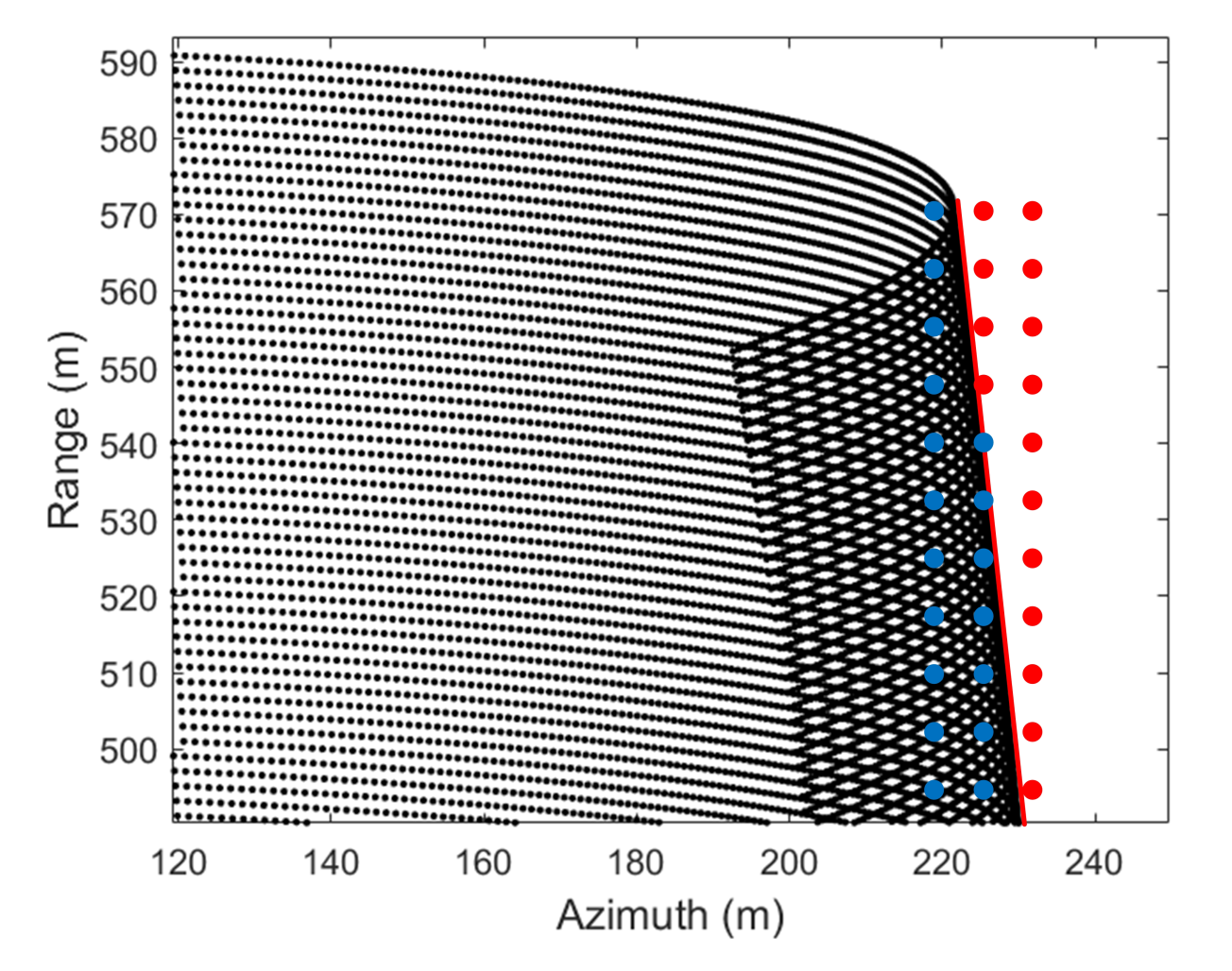
4. Swath Limit Analysis

The precision of the proposed ML-OSA is evaluated by using the swath limit in a given resolution level. The factors affecting the swath limit includes the signal model accuracy, the borderline of the folding phenomenon and the residual phase error of multi-level compensation, as follows:

4.1. Signal Model Accuracy

The accuracy of signal approximation model described in (10) is the basis of the ML-OSA. For each scatterer in the swath, their phase errors $\Delta {\Phi }_{\mathrm{model}}$ between the approximation model and the real echo signal can be calculated by the following formula. When the maximum value of $\Delta {\Phi }_{\mathrm{model}}$ is less than the threshold of $\pi /4$, the signal approximation model can represent the real echo signal precisely. Generally speaking, the longer distance between the target and the scene center, the more serious its phase error will be. Therefore, the swath limit for the model is required to provide firstly.

$$\Delta {\Phi }_{\mathrm{model}}(i,m)=\left|S_3(i,m)-S_4(i,m)\right|$$

(39)

where $S_3(i,m)$ and $S_4(i,m)$ are represented by the phase of (9) and (10), respectively.

The proposed signal model in (10) shows much higher accuracy than the existing signal model in [16]. Based on the parameters listed in Table 1, the theoretical swath limits of two signal models are drawn in Figure 10, where the swath limit of the proposed signal model is denoted by the solid contour line and the swath limit of the existing signal model is represented by the dotted one. The solid contour line is drawn by the scatterers whose maximum values of $\Delta {\Phi }_{\mathrm{model}}$ are equal to $\pi /4$. However, the swath limit of existing signal model only considers the QPE because the previous OSA in [16] did not use the linear phase for compensation processing. Thus, the dotted contour line denotes the maximum QPEs of $\pi /4$ in the swath. The swath limit of proposed model is about 4.8 times larger than that of model in [16].

The image qualities of the two signal models are further compared via the point-target simulation in Figure 11, where three points are drawn in Figure 10. Point 1 is inside the swath limit of two models with the coordinate (−200, −260), while Point 2 is inside the limit of proposed model but outside the limit of existing model with the coordinate (−320, −250). Point 3 is outside the two limits and its coordinate is (−320, −550). Though the performance of other scatterers may differ slightly with respect to these selected points, they share the same trend. In particular, to analyze the model accuracy exactly, the filters of two models (such as $exp(-j{U}_3{K}_{\mathrm{x}}^{\prime 2}\left(m\right))$ in (11)) are directly generated to compensate the QPE, respectively.

The azimuth profiles processed by two models of these targets are drawn in Figure 11 to examine the their target-focusing qualities. The range profiles are not presented because the image quality degradation occurs merely along the azimuth dimension. It can be found from Figure 11a that the Point 1 within the two swath limits is well-focused. The image result of Point 2 in Figure 11b shows that the proposed model is better than the model in [16]. The image quality of Point 3 processed by two models are unsatisfactory as expected because it is outside the accuracy of the two signal models. This simulation confirms the superiority of the proposed signal approximation model.

4.2. Folding Phenomenon in Subaperture Compensation Generation

In the subaperture compensation generation, an important step is to solve the real coordinates from the distorted coordinates. However, the equation in (A21) for solving the real target coordinates has two solutions as in (A23), and sometimes the equation has no solution. The case of two solutions means that the two real coordinates have the same distorted coordinate. As shown in Figure 12, the black points are part of the coordinates of the real coordinate point matrix after geometric distortion. It can be seen that some distorted coordinates are folded and coincided with other coordinates, which explains why the equation has two solutions. Besides, this phenomenon is called the folding phenomenon of distorted coordinates. Unfortunately, this situation causes data overlap and affects subsequent GDC processing. Therefore, it is necessary to find the borderline to avoid folding phenomenon in the imaging swath. In addition, the right side of distorted azimuth coordinates has maximum values (the red line in Figure 12) due to the folding phenomenon. When compensating the phase error by subaperture estimation, each distorted azimuth coordinate will correspond to an azimuth measured value (such as ${\rho }_{{\mathrm{x}}_1}{m}_1^{\prime }$ in (20) and ${\rho }_{{\mathrm{x}}_1}{m}_1^{\prime }+{\rho }_{{\mathrm{x}}_2}{m}_2^{\prime }$ in (25)). The blue and red points in Figure 12 represent different measured values. If some measured values are bigger than the maximum values of distorted azimuth coordinates (as shown by the red points in Figure 12), the equation in (A21) has no solution because there are no real coordinates corresponding to these measured values.

In order to locate the borderline of folding phenomenon, the algorithm-based analysis is conducted firstly. From the first order coefficients given by (A10), each real point coordinate $(x_{\mathrm{p}},y_{\mathrm{p}})$ corresponds to a geometric distorted coordinate $(x_{\mathrm{p}}+U_2,y_{\mathrm{p}}+U_1)$. Furthermore, it is generally considered that the azimuth coordinate of the distortion position $x_{\mathrm{p}}+U_2$ increases with the increasing $x_{\mathrm{p}}$ for a certain $y_{\mathrm{p}}$. However, as shown in Figure 12, the distortion coordinates have the folding phenomenon, which shows that $x_{\mathrm{p}}+U_2$ is not always proportional to $x_{\mathrm{p}}$. The derivative $\partial \left(x_{\mathrm{p}}+U_2\left(x_{\mathrm{p}},y_{\mathrm{p}}\right)\right)/\partial x_{\mathrm{p}}$ is no longer always bigger than 0, but sometimes less than 0. Thus, the borderline of the folding phenomenon can be calculated by the following formula. Besides, the imaging range should be selected on the side of the borderline to ensure that $x_p+U_2\left(x_{\mathrm{p}},y_{\mathrm{p}}\right)$ varies monotonously for each $y_{\mathrm{p}}$.

$$\frac{\partial \left(x_{\mathrm{p}}+U_2\left(x_{\mathrm{p}},y_{\mathrm{p}}\right)\right)}{\partial x_{\mathrm{p}}}=0$$

(40)

When the squint angle is large enough, the extension line of the projection of the sensor linear flight trajectory on the XOY plane, as shown by the red dotted line in the Figure 13a, passes through the specified imaging scene. Obviously, two scatterers which are symmetric about the red dotted line have the same slant range history and phase. They have the same linear term and quadratic term and hence the folding phenomenon will appear. This red dotted line is the borderline of folding phenomenon and can be obtained by (41). The borderlines drawn by (40) and (41) are the same, so the folding phenomenon is verified by both algorithm and mechanism.

$$y_{\mathrm{p}}=-\frac{x_{\mathrm{p}}}{tan\delta }+Htan{\beta }_0$$

(41)

If the imaging area contains the scatterers which are symmetric about the borderline, their energy will be undesirably mixed together in the image. Therefore, the imaging range should be selected on the one side of the borderline. Usually, the imaging area includes the scene center, so the left side of the borderline is selected. Figure 13b represents the imaging area on the ground plane, where the red dotted line is the boundary of folding phenomenon and the yellow area denotes the selected imaging range. However, sometimes the antenna irradiation region will include the borderline just like the whole square area in Figure 13b. The area surrounded by the dashed frame and the blue area are symmetric about the red line. In this case, these two regions will be focused together in the image. Besides, it is hard to accurately restore the respective information of the scattering points in these two areas during GDC. Thus, the effective swath limit is the yellow region except the dotted frame area.

By employing the simulation parameters listed in Table 1 and the formula written in (40) or (41), we can draw the borderline in Figure 14a, where the straight line represents the borderline and the contour line is the swath limit for the signal model. As is shown in Figure 14a, Point 4 and Point 5 are both inside the swath limit and are symmetrical about the borderline with coordinates (322.8, 399.3) and (599.2, 428.4), respectively. Therefore, these two points have the same geometric distortion coordinate.

The simulation for these two scatterers is processed by parameter-adjusting the ML-OSA with the layer of two, Figure 13b is the SAR imaging result and Figure 13c represents the two-dimensional PSF of the focused point. It shows that two different point-targets are well-focused together with the coordinate (216.6, 385) due to the PWA. This simulation verifies not only the folding phenomenon of the distortion coordinate, but also the accuracy of the borderline. In order to avoid this phenomenon, the effective imaging area should be on the one side of the borderline. Generally speaking, the imaging range should include the scene center, so the left side of the borderline is selected in the subsequent research.

4.3. Residual Phase Error of the ML-OSA

For the residual phase error of ML-OSA, its swath limits are not only determined by the QPE limits of each azimuth dimension, such as (16), (23), (29), but also related to the migration limits, such as (19), (24). Therefore, the swath limits for residual phase error of ML-OSA can be written as the following two categories.

The QPE limits:

$$\left|U_3\left(x_{\mathrm{p}},y_{\mathrm{p}}\right)\right|<{\displaystyle \frac{{\rho }_{{\mathrm{x}}_1}^2}{4\pi }},\left|U_3\left(x_{\mathrm{p}},y_{\mathrm{p}}\right)-{\widehat{U}}_3^{\left(1\right)}\left(x_{\mathrm{p}},y_{\mathrm{p}}\right)\right|<{\displaystyle \frac{{\rho }_{{\mathrm{x}}_2}^2}{4\pi }},\cdots ,\left|U_3\left(x_{\mathrm{p}},y_{\mathrm{p}}\right)-{\widehat{U}}_3^{\left(\mathrm{N}\right)}\left(x_{\mathrm{p}},y_{\mathrm{p}}\right)\right|<{\displaystyle \frac{{\rho }_{{\mathrm{x}}_{\mathrm{N}+1}}^2}{4\pi }}$$

(42)

The migration limits:

$$\left|U_3\left(x_{\mathrm{p}},y_{\mathrm{p}}\right)\right|<{\displaystyle \frac{{\rho }_{{\mathrm{x}}_1}{\rho }_{{\mathrm{x}}_{\mathrm{N}+1}}}{4\pi }},\left|U_3\left(x_{\mathrm{p}},y_{\mathrm{p}}\right)-{\widehat{U}}_3^{\left(1\right)}\left(x_{\mathrm{p}},y_{\mathrm{p}}\right)\right|<{\displaystyle \frac{{\rho }_{{\mathrm{x}}_2}{\rho }_{{\mathrm{x}}_{\mathrm{N}+1}}}{4\pi }},\cdots ,\left|U_3\left(x_{\mathrm{p}},y_{\mathrm{p}}\right)-{\widehat{U}}_3^{(\mathrm{N}-1)}\left(x_{\mathrm{p}},y_{\mathrm{p}}\right)\right|<{\displaystyle \frac{{\rho }_{{\mathrm{x}}_{\mathrm{N}}}{\rho }_{{\mathrm{x}}_{\mathrm{N}+1}}}{4\pi }}$$

(43)

According to the principle of subaperture division, it can be concluded that ${\rho }_{{\mathrm{x}}_1}>{\rho }_{{\mathrm{x}}_2}>\cdots >{\rho }_{{\mathrm{x}}_{\mathrm{N}+1}}$. Comparing the first inequality in (42) and (43), the former inequality can be neglected, because ${\rho }_{{\mathrm{x}}_1}>{\rho }_{{\mathrm{x}}_{\mathrm{N}+1}}$. By analogy, all inequalities except the last one in (42) can be ignored. Thus, the swath limits for residual phase error of ML-OSA becomes

$$\begin{array}{c}\hfill \left\{\begin{array}{c}\left|U_3\left(x_{\mathrm{p}},y_{\mathrm{p}}\right)-{\widehat{U}}_3^{\left(\mathrm{N}\right)}\left(x_{\mathrm{p}},y_{\mathrm{p}}\right)\right|<{\displaystyle \frac{{\rho }_{{\mathrm{x}}_{\mathrm{N}+1}}^2}{4\pi }},\left|U_3\left(x_{\mathrm{p}},y_{\mathrm{p}}\right)\right|<{\displaystyle \frac{{\rho }_{{\mathrm{x}}_1}{\rho }_{{\mathrm{x}}_{\mathrm{N}+1}}}{4\pi }}\hfill \\ \left|U_3\left(x_{\mathrm{p}},y_{\mathrm{p}}\right)-{\widehat{U}}_3^{\left(1\right)}\left(x_{\mathrm{p}},y_{\mathrm{p}}\right)\right|<{\displaystyle \frac{{\rho }_{{\mathrm{x}}_2}{\rho }_{{\mathrm{x}}_{\mathrm{N}+1}}}{4\pi }},\cdots ,\left|U_3\left(x_{\mathrm{p}},y_{\mathrm{p}}\right)-{\widehat{U}}_3^{(\mathrm{N}-1)}\left(x_{\mathrm{p}},y_{\mathrm{p}}\right)\right|<{\displaystyle \frac{{\rho }_{{\mathrm{x}}_{\mathrm{N}}}{\rho }_{{\mathrm{x}}_{\mathrm{N}+1}}}{4\pi }}\hfill \end{array}\right.\end{array}$$

(44)

The first inequality in (44) denotes the QPE limit and the others are the migration limits. More subaperture layers allow larger QPE-limited swath. However, when the number of layers N is large enough, the remaining migration items will restrict the swath. Thus, the swath is limited by all the inequalities described in (44).

The performance of the two-layer ML-OSA (an example of ML-OSA) is compared with zero-layer ML-OSA (i.e., parameter-adjusting PFA) and one-layer ML-OSA (a special case of ML-OSA) by a simulated Ka-band EHS HRWS parameter-adjusting SAR. The ground range and azimuth resolutions are both set as 0.3 m and the key simulation parameters are listed in Table 1. Based on the derivations described in (44), the swath limits for the residual phase error of zero-layer, one-layer and two-layer ML-OSA are drawn in Figure 15 with black dotted, blue and red contour line, respectively. As shown in Figure 15, the black contour line and black straight line denote the borderline and the swath limit for the signal model, which are the basic constraints of the imaging scene. Moreover, the area surrounded by the green dotted border represents the region for the second extended-target simulation in Section 6. In addition, the grey area in Figure 15 is the domain where the equation in (A21) has no solution, as explained in Section 4.2. One-layer and two-layer ML-OSA have the subaperture compensation process, so the swath limits for them cannot contain the gray area.

By considering the borderline and the signal model accuracy, the swath limits of the three algorithms are surrounded by the respective contour line, which are depicted in Figure 16. The edge of the swath limit for one-layer ML-OSA is jagged shown in Figure 16b, owing to the fact that the low accuracy of one-layer ML-OSA coarse estimation compensation in these area. One-layer and two-layer ML-OSA contributes to 5.1 times and 6.2 times larger swath than the zero-layer ML-OSA. Compared with the swath limit of one-layer ML-OSA, the swath limit of two-layer ML-OSA is increased by about 21%.

To verify the performance difference between one-layer and two-layer ML-OSA, two scatterers are chosen as examples for simulation and their distribution is shown in Figure 15. These two targets are all within the swath limits for signal model accuracy and two-layer ML-OSA and locate on the left side of the borderline. Point 6 is inside the swath limit for one-layer ML-OSA with coordinate (290, 130), while Point 7 is outside the swath limit for one-layer ML-OSA with coordinate (270, 450). In particular, the azimuth profiles of two scatterers are presented in Figure 17 , where the dotted profiles represent the results of one-layer ML-OSA and the solid ones denote the results of two-layer ML-OSA. The range profiles are not presented since QPE is merely along the azimuth dimension. It is found that for the scatterer that is within the swath limit of the one-layer ML-OSA, two algorithms contribute to acceptable results. However, for the Point 7 that is outside the swath limit of one-layer ML-OSA but inside the swath limit of the two-layer ML-OSA, the difference between two algorithms are significant. The result of Point 7 processed by the one-layer ML-OSA is defocused and the PSLR is about −8 dB, while the two-layer ML-OSA still contributes to good focusing result and the PSLR is better than −13 dB. This point-target simulation confirms the superiority of multi-layer compensation and also verifies the swath limits in Figure 15.

5. Discussion

The proposed parameter-adjusting method is different with the motion compensation (MoCo). The mechanism of MoCo is to use the trajectory data to compensate the echo collected by the non-ideal trajectory into the echo under the ideal trajectory [42,43]. Thus, the function of MoCo is to correct the influence of non-ideal trajectory on the echoed data. Some radar systems make the echoed signal uniformly sampled along the azimuth direction by adjusting the pulse repeat frequency. However, the parameter-adjusting method has different function. Its function is to correct the distorted wavenumber spectrum and the distortion of PSF to improve the resolution performance. In parameter-adjusting case, the range interpolation, which is necessary in the constant-parameter PFA to convert data from polar format to keystone format, can be eliminated. Therefore, parameter-adjusting method can also improve the processing efficiency.

In practical applications, the non-ideal trajectory and the precise of parameter adjustment will affect the imaging effect of the proposed algorithm. The non-ideal trajectory is caused by the motion error of the sensor [42,43]. In this section, the non-ideal trajectory is to be discussed from the motion error that can be accurately measured and the motion error that cannot be accurately measured. Due to hardware limit, the radar parameter adjustment is approximately converted from pulse-by-pulse to segment-to-segment manner, which leads to inaccurate parameter adjustment.

5.1. Measurable Motion Error

Assume that the SAR platform moves with some deviation from the planned, e.g., rectilinear, trajectory and this deviation can be accurately measured by a high-accurate integrated navigation system. The ideal rectilinear trajectory $\left(x\right(t),y(t),z(t\left)\right)$ is written in (A2). By assuming a sine error in the ideal trajectory, the real trajectory yields

$$x_{\mathrm{r}}\left(t\right)=x\left(t\right)+A_{1}sin\left(2\pi {\displaystyle \frac{t}{T_{\mathrm{syn}}}}\right)y_{\mathrm{r}}\left(t\right)=y\left(t\right)+A_{2}sin\left(2\pi {\displaystyle \frac{t}{T_{\mathrm{syn}}}}\right)z_{\mathrm{r}}\left(t\right)=z\left(t\right)+A_{3}sin\left(2\pi {\displaystyle \frac{t}{T_{\mathrm{syn}}}}\right)$$

(45)

where $(x_{\mathrm{r}}\left(t\right),y_{\mathrm{r}}\left(t\right),z_{\mathrm{r}}\left(t\right))$ represents the ideal trajectory with sine error and $A_1$, $A_2$, $A_3$ are the coefficients of sine error. The geometry of extremely-high-squint SAR with motion error is shown in Figure 18, where the solid and dotted blue line indicate the ideal trajectory with error and without error, respectively.

According to the real trajectory with measurable sine errors, the carrier frequency and chirp rate are adjusted as

$$f_{\mathrm{cr}}\left(m\right)=f_{\mathrm{c}0}{\displaystyle \frac{sin{\beta }_0}{sin{\beta }_{\mathrm{r}}\left(m\right)cos{\alpha }_{\mathrm{r}}\left(m\right)}}{\gamma }_{\mathrm{r}}\left(m\right)={\gamma }_0{\displaystyle \frac{sin{\beta }_0}{sin{\beta }_{\mathrm{r}}\left(m\right)cos{\alpha }_{\mathrm{r}}\left(m\right)}}$$

(46)

where ${\beta }_{\mathrm{r}}$ and ${\alpha }_{\mathrm{r}}$ are determined by the real trajectory. After the operations of two-dimensional dechirping and RVP removal, the signal yields

$$S_{\mathrm{r}}(i,m)=exp\left\{j{\displaystyle \frac{4\pi }{c}}\left(f_{\mathrm{c}\mathrm{r}}\left(m\right)+{\displaystyle \frac{{\gamma }_{\mathrm{r}}\left(m\right)}{F_s}}i\right)\left(R_{\mathrm{c}\mathrm{r}}\left(m\right)-R_{\mathrm{p}\mathrm{r}}\left(m\right)\right)\right\}$$

(47)

where

$$R_{\mathrm{c}\mathrm{r}}\left(m\right)-R_{\mathrm{p}\mathrm{r}}\left(m\right)=\sqrt{{\left(x_{\mathrm{r}}-x_{\mathrm{p}}\right)}^2+{\left(y_{\mathrm{r}}-y_{\mathrm{p}}\right)}^2+{\left(z_{\mathrm{r}}-z_{\mathrm{p}}\right)}^2}-\sqrt{x_{\mathrm{r}}^2+y_{\mathrm{r}}^2+z_{\mathrm{r}}^2}$$

(48)

By employing the parameter-adjusting method in (46), the wavenumber spectrum can be guaranteed to be the keystone format and thus the range interpolation can be eliminated. After the azimuth interpolation, the signal can be expressed as

$$S_{\mathrm{r}}(i,m)\approx exp\left\{j\left(x_{\mathrm{p}}{K}_{\mathrm{x}}^{\prime }\left(m\right)+y_{\mathrm{p}}{K}_{\mathrm{y}}^{\prime }\left(i\right)\right)\right\}exp\left\{j\left(B_1{K}_{\mathrm{x}}^{\prime }\left(m\right)+B_2{K}_{\mathrm{x}}^{\prime 2}\left(m\right)+B_3{K}_{\mathrm{x}}^{\prime 3}\left(m\right)+B_4{K}_{\mathrm{x}}^{\prime 4}\left(m\right)+C_1{K}_{\mathrm{y}}^{\prime }\left(i\right)\right)\right\}$$

(49)

Since the motion error is sine format in (45), the starting and ending positions of the ideal trajectory and the real trajectory are the same, and thus the interpolated range and azimuth wavenumber ($K_{\mathrm{y}}^{\prime }\left(i\right)$ and $K_{\mathrm{x}}^{\prime }\left(m\right)$) in (49) can be expressed as (12). Therefore, the phase in (11) can be employed to compensate the phase error of trajectory with motion error. The following part analyzes the impact of such compensation.

When the quadratic phase $U_3{K}_{\mathrm{x}}^{\prime 2}\left(m\right)$ for ideal trajectory in (11) is employed to compensate the quadratic phase error $B_2{K}_{\mathrm{x}}^{\prime 2}\left(m\right)$ in (49) for real trajectory, the new quadratic phase error (NQPE) $(B_2-U_3)K_{\mathrm{x}}^{\prime 2}\left(m\right)$ will affect the image focus. If the NQPE exceeds the threshold of $\pi /4$, it will cause the defocus along the azimuth direction. Different from the signal model in (11), the cubic and quartic terms of azimuth wavenumber need to be considered due to the trajectory error. When the cubic phase error $B_3{K}_{\mathrm{x}}^{\prime 3}\left(m\right)$ exceeds the threshold of $\pi /8$ or the quartic phase error $B_4{K}_{\mathrm{x}}^{\prime 4}\left(m\right)$ is higher than $\pi /16$, the sidelobe will be affected. Therefore, the influence of NQPE, cubic phase error and quartic phase error should be considered when the trajectory error is occurred.

According to the simulation parameters in Table 1, the case in which the trajectory error coefficients $A_1$, $A_2$, $A_3$ are 1 is simulated and analyzed. The coefficients $B_2$, $B_3$, $B_4$ in (49) are calculated by fitting $K_{\mathrm{x}}^{\prime }\left(m\right)$ to the interpolated phase. Based on (50), the theoretical swath limits for NQPE, cubic and quartic phase error are drawn in Figure 19, where they are denoted by the red, blue and black contour line. It shows that the swath limit of NQPE is bigger than the swath limits of cubic and quartic phase error.

$$\left|\left(B_2-U_3\right)K_{\mathrm{x}}^{\prime 2}\left(m\right)\right|\le {\displaystyle \frac{\pi }{4}}\left|B_3{K}_{\mathrm{x}}^{\prime 3}\left(m\right)\right|\le {\displaystyle \frac{\pi }{8}}\left|B_4{K}_{\mathrm{x}}^{\prime 4}\left(m\right)\right|\le {\displaystyle \frac{\pi }{16}}$$

(50)

Three scatterers are chosen as examples for simulation and their distribution is shown in Figure 19. Point 8 is within the three limits with the coordinate (0, 60), Point 9 is outside the swath limits of cubic and quartic phase error but inside the limit of NQPE with the coordinate (60, 60), and Point 10 is outside all limits with the coordinate (120, 120). The filter is directly generated according to the $U_3{K}_{\mathrm{x}}^{\prime 2}\left(m\right)$ in (11) to compensate for the phase error in the real trajectory. The imaging results including the two-dimensional PSFs and azimuth profiles are shown in Figure 20. It can be seen from Figure 20a that Point 8 is well-focused as expected. The sidelobe of Point 9 in Figure 20b is raised due to the influence of the cubic and quartic phase error. The two-dimensional PSF of Point 10 in Figure 20c is defocused. This simulation confirms that the influence of NQPE, cubic phase error and quartic phase error should be considered when the trajectory has motion error.

5.2. Unmeasurable Motion Error

Similar to Section 5.1, it is still assume that the SAR platform moves with some deviation from the planned, e.g., rectilinear, trajectory. But in this case, this deviation cannot be accurately measured due to insufficient accuracy of the integrated navigation system. As a result, the radar-parameter are adjusted based on the ideal path instead of the real path.

Still assuming that there is a sine error in the trajectory, the expression of real trajectory is written in (45). The carrier frequency and chirp rate are adjusted based on the ideal trajectory as (7). Since the real slant range distance history of scene center $R_{\mathrm{pr}}\left(m\right)$ cannot be obtained, the ideal slant range history of scene center $R_{\mathrm{p}}\left(m\right)$ is used for the dechirp processing. Afterwards, the signal after two-dimensional dechirping and RVP removal can be expressed as

$$S_{\mathrm{rr}}(i,m)=exp\left\{j{\displaystyle \frac{4\pi }{c}}\left(f_{\mathrm{c}}\left(m\right)+{\displaystyle \frac{\gamma \left(m\right)}{F_s}}i\right)\left(R_{\mathrm{c}\mathrm{r}}\left(m\right)-R_{\mathrm{p}}\left(m\right)\right)\right\}$$

(51)

It can be seen from (51) that the slant range history of the scene center has not been accurately compensated. This leads to the imaging defocus at the scene center. As the trajectory motion error increases, the defocusing phenomenon becomes more serious. Therefore, autofocus processing is needed, but it is not the focus of this paper.

In order to prove the above analysis, the point target simulation is conducted at scene center with the parameters in Table 1 and different trajectory error coefficients ($A_1$ = $A_2$ = $A_3$ = 0.001, $A_1$ = $A_2$ = $A_3$ = 0.01, $A_1$ = $A_2$ = $A_3$ = 0.02). The imaging results are shown in Figure 21. It shows that the defocus phenomenon becomes more serious as the motion error coefficient increases. Figure 22 is the image of employing the traditional autofocus processing (Phase Gradient Autofocus [44]). The two-dimensional PSFs of the first two cases in Figure 22a,b are well-focused but the PSF of the last case in Figure 22c is a little bit defocused. Therefore, the autofocus method may be further studied in future research.

5.3. Segment-by-Segment Parameter Adjustment

Restricted by hardware ability, it is practically hard to adjust radar parameters in a pulse-by-pulse manner. Alternatively, it is more feasible to adjust radar parameters segment-by-segment, meaning that during a couple of pulses the radar parameters are unchanged. In this case, assume the carrier frequency and chirp rate are adjusted segment-by-segment as

$$f_{\mathrm{c}\mathrm{s}}\left(m\right)=f_{\mathrm{c}}\left(\left(⌈{\displaystyle \frac{m}{M_{\mathrm{s}}}}⌉-1\right)M_{\mathrm{s}}+1\right){\gamma }_{\mathrm{s}}\left(m\right)=\gamma \left(\left(⌈{\displaystyle \frac{m}{M_{\mathrm{s}}}}⌉-1\right)M_{\mathrm{s}}+1\right)$$

(52)

where $M_{\mathrm{s}}$ represents the segment length and $⌈·⌉$ depicts the rounding up function. $f_{\mathrm{c}}\left(m\right)$ and $\gamma \left(m\right)$ are the continuously varying carrier frequency and chirp rate written in (7). In this case, the segment-varying carrier frequency $f_{\mathrm{cs}}\left(m\right)$ and chirp rate ${\gamma }_{\mathrm{s}}\left(m\right)$ are distributed in steps along the azimuth time. The signal after pre-processing yields

$$S_{\mathrm{s}}(i,m)=exp\left\{j{\displaystyle \frac{\sqrt{K_{\mathrm{x}\mathrm{s}}^2(i,m)+K_{\mathrm{y}\mathrm{s}}^2(i,m)}}{sin\beta \left(m\right)}}\left(R_{\mathrm{c}}\left(m\right)-R_{\mathrm{p}}\left(m\right)\right)\right\}$$

(53)

where

$$\begin{array}{c}\hfill \left\{\begin{array}{cc}& K_{\mathrm{xs}}(i,m)={\displaystyle \frac{4\pi }{c}}\left(f_{\mathrm{cs}}\left(m\right)+{\displaystyle \frac{{\gamma }_{\mathrm{s}}\left(m\right)}{F_{\mathrm{s}}}}i\right)sin\beta \left(m\right)sin\alpha \left(m\right)\\ & K_{\mathrm{ys}}(i,m)={\displaystyle \frac{4\pi }{c}}\left(f_{\mathrm{cs}}\left(m\right)+{\displaystyle \frac{{\gamma }_{\mathrm{s}}\left(m\right)}{F_{\mathrm{s}}}}i\right)sin\beta \left(m\right)cos\alpha \left(m\right)\end{array}\right.\end{array}$$

(54)

According to the derivation in Appendix B, the signal model of segment-varying parameters can be expressed as

$$S_{\mathrm{s}}(i,m)\approx exp\left\{j\left(\left(y_{\mathrm{p}}+U_1\right)K_{\mathrm{ys}}+\left(x_{\mathrm{p}}+U_2\right)K_{\mathrm{xs}}+U_3{K}_{\mathrm{xs}}^2\right)\right\}$$

(55)

where the expressions of $U_1$, $U_2$ and $U_3$ are same as (A12). The method of segment-varying parameters does not cause additional image defocusing because the coefficients $U_1$, $U_2$ and $U_3$ are constants for a certain target. Therefore, the ML-OSA can be directly used to compensate for the defocus originally caused by the planar wavefront assumption. However, the segment-varying parameter method may cause spurious targets along the azimuth direction.

Based on the simulation parameters in Table 1, the point target simulation is conducted with segment-varying parameters of different segment lengths. The point target is placed at (320, 320) and the radar parameters i.e., carrier frequency and chirp rate are adjusted every 100, 500 and 1000 pulses. The variation of carrier frequency and chirp rate are depicted in Figure 23. The blue lines represent the continuously time-varying parameters and the red lines are the segment-varying parameters. The wavenumber spectrums and two-dimensional PSFs processed by two-layer ML-OSA are shown in Figure 24. It shows that the sawtooth shape on both sides of the wavenumber spectrum becomes more serious with the segment length increases. Besides, spurious targets appear in Figure 24b,c because of the long segmentation. This simulation confirms that the proposed algorithm can be applied with the segment-varying parameters when the segment length is within a certain threshold.

6. Extended-Target Simulations

The extended-target simulations are based on the ideal case (without considering any errors) and the non-ideal case (with considering the motion error or the precise of parameter adjustment).

6.1. Ideal Case

In order to further analyze the superiority of the parameter-adjusting method, the first simulation is performed for a small scene size (40 m × 40 m). The ground range and azimuth resolutions are both set as 0.3 m and the other parameters are listed in Table 1 where the squint angle is 80.9${}^{\circ }$. The carrier frequency varies from 30.11 GHz to 29.83 GHz and the chirp rate ranges from 54.23 THz/s to 53.74 THz/s as shown in Figure 5a,b. Two adjacent point-targets are placed at the upper left corner of the extended-target to verify the imaging performance. And the distance between these two targets is about 0.27 m. The imaging results processed by two-layer ML-OSA with the constant-parameter and parameter-adjusting method are illustrated in Figure 25a and Figure 25b respectively. In these two pictures, the small images in the middle are the zoomed-in views of the two close point-targets. As shown in the zoomed-in figures, two points can be easily discriminated by the proposed method, while they are mixed together by the constant-parameter method. This simulation proves that the parameter-adjusting method have the advantage of improving the target discrimination performance.

The second simulation chooses the area surrounded by the green frame in Figure 15 to verify the imaging performance of ML-OSA under EHS HRWS parameter-adjusting SAR. The coverage of the scene is 640 m × 640 m and the two-dimensional ground resolutions are 0.3 m × 0.3 m. The other parameters are also listed in Table 1 where the squint angle is 80.9${}^{\circ }$. The carrier frequency varies from 30.11 GHz to 29.83 GHz and the chirp rate ranges from 54.23 THz/s to 53.74 THz/s. Two strong point scatterers are placed on the upper and lower edges of the scene with the coordinates (−152, 308) and (−267, −312), respectively. Besides, this area is within the swath limit of model accuracy and on the left side of the borderline. So only the swath limits of these three algorithms needs to be considered in this imaging scene.

The simulation results of zero-layer, one-layer, two-layer ML-OSA and BPA are shown in Figure 26, where the geometrical distortion has been corrected via the cubic interpolation based on (A10). The yellow contour lines drawn in Figure 26a–d denote the swath limits of zero-layer, one-layer, two-layer ML-OSA and BPA respectively. To observe their imaging difference clearly, the two-dimensional impulse response functions of two scatterers are depicted in the middle of them. It shows that the imaging result of zero-layer ML-OSA is significantly worse than the other three algorithms. The image focused by one-layer ML-OSA are not as well as two-layer ML-OSA at the edges of the scene. Inspecting the PSFs drawn in Figure 26b,c, it can be seen from these PSFs that the imaging performance of two-layer ML-OSA is better than one-layer ML-OSA. To further make the comparison solid, the result of two-layer ML-OSA and BPA (Figure 26c,d) are compared. By showing that proposed method leads to an equivalent image quality with that achieved by the BPA, the effectiveness of presented approach is proved in a more concrete way.

6.2. Non-Ideal Case

The first simulation of the non-ideal cases assumes that the trajectory has a measurable motion error. The trajectory with the sine error is described in (45) and the sine error coefficients $A_1$, $A_2$, $A_3$ are simulated with two cases. One is small-error case with $A_1$ = $A_2$ = $A_3$ = 0.05 and the other is large-error case with $A_1$ = $A_2$ = $A_3$ = 1. The coverage of the imaging scene is 640 m × 640 m and the other parameters are listed in Table 1. Two strong point scatterers are placed in the scene with the coordinates (10, −25) and (−45, −208). The images processed by two-layer ML-OSA of two cases are shown in Figure 27a,d. The yellow contour lines denote the swath limits of them, respectively. From the two-dimensional impulse response functions in Figure 27a,d, it can be seen that the imaging result with $A_1$ = $A_2$ = $A_3$ = 0.05 is better than the image with $A_1$ = $A_2$ = $A_3$ = 1 as expected.

Based on the unmeasurable motion error analyzed in Section 5.2, the second simulation is conducted with the unmeasurable error with the coefficients $A_1$ = $A_2$ = $A_3$ = 0.02. The main parameters are shown in Table 1. To compare the direct imaging result with the autofocus imaging result, a strong scatterer is placed in the scene with the coordinate (−45, −208). The imaging results of direct two-layer ML-OSA imaging and autofocus imaging (via estimating residual trajectory deviations [45]) are drawn in Figure 27b and Figure 27e, respectively. It shows that the extended-target image in Figure 27b is severely defocused and the image after autofocus in Figure 27e is improved.

The third simulation is conducted with the segment-by-segment parameter adjustment. The segment-varying carrier frequency and chirp rate are written in (52) and this simulation includes two cases (parameters are adjusted every 100 pulses and 1000 pulses). The coverage of the imaging scene is 640 m × 640 m and the other parameters are shown in Table 1 and two strong point scatterers are placed on the upper and lower edges of the scene with the coordinates (−152, 308) and (−267, −312), respectively. The images processed by two-layer ML-OSA of segment-varying parameter are shown in Figure 27c,f. To observe their imaging difference clearly, the two-dimensional impulse response functions of two scatterers are depicted in the middle of the extended-target images. It shows that the spurious targets appear in Figure 27f because of the long segmentation.

7. Conclusions

In this paper, a ML-OSA algorithm has been proposed for EHS HRWS parameter-adjusting SAR imaging. Comparing to the existing parameter-adjusting SAR algorithm, the ML-OSA contributes to much higher accuracy by employing a much more accurate signal model for spatially variant phase error description and a much more accurate multi-layer phase compensation strategy for spatially phase error compensation. Specifically, the reason for the former is the complete expansion of two-dimensional Taylor series and the reason for the latter is the employment of a more accurate way to generate spatially variant phase error compensators. The presented approach has been evaluated by the computer simulations, showing that the accuracy of proposed parameter-adjusting signal model is 4.8 times higher than the existing parameter-adjusting signal model and that one-layer and two-layer ML-OSA contributes to 5.1 times and 6.2 times larger swath than the existing parameter-adjusting PFA. Future work will focus on analyzing the autofocus method and applying the proposed algorithm to real SAR systems.

References

1. Carrara, W.G.; Goodman, R.S.; Majewski, R.M. Spotlight Synthetic Aperture Radar: Signal Processing Algorithms; Artech House: Boston, MA, USA, 1995. [Google Scholar]
2. Lin, Y.; Hong, W.; Li, Y.; Tan, W.; Yu, L.; Hou, L.; Wang, J.; Liu, Y.; Wang, W. Study on fine feature description of multi-aspect SAR observations. In Proceedings of the 2016 IEEE International Geoscience and Remote Sensing Symposium (IGARSS), Beijing, China, 10–15 July 2016; pp. 5682–5685. [Google Scholar]
3. Chen, S.; Yuan, Y.; Zhang, S.; Zhao, H.; Chen, Y. A New Imaging Algorithm for Forward-Looking Missile-Borne Bistatic SAR. IEEE J. Sel. Top. Appl. Earth Obs. Remote Sens. 2016, 9, 1543–1552. [Google Scholar] [CrossRef]
4. Zeng, T.; Li, Y.; Ding, Z.; Long, T.; Yao, D.; Sun, Y. Subaperture Approach Based on Azimuth-Dependent Range Cell Migration Correction and Azimuth Focusing Parameter Equalization for Maneuvering High-Squint-Mode SAR. IEEE Trans. Geosci. Remote Sens. 2015, 53, 6718–6734. [Google Scholar] [CrossRef]
5. Zhou, Z.; Ding, Z.; Zhang, T.; Wang, Y. High-Squint SAR Imaging for Noncooperative Moving Ship Target Based on High Velocity Motion Platform. In Proceedings of the 2018 China International SAR Symposium (CISS), Shanghai, China, 10–12 October 2018; pp. 1–5. [Google Scholar]
6. Xu, X.; Su, F.; Gao, J.; Jin, X. High-Squint SAR Imaging of Maritime Ship Targets. IEEE Trans. Geosci. Remote Sens. 2020, 60, 1–16. [Google Scholar] [CrossRef]
7. Davidson, G.; Cumming, I. Signal properties of spaceborne squint-mode SAR. IEEE Trans. Geosci. Remote Sens. 1997, 35, 611–617. [Google Scholar] [CrossRef] [Green Version]
8. Beard, G.S. Performance Factors for Airborne Short-Dwell Squinted Radar Sensors. Ph.D. Thesis, UCL (University College London), London, UK, 2011. [Google Scholar]
9. Zhang, Q.; Yin, W.; Ding, Z.; Zeng, T.; Long, T. An Optimal Resolution Steering Method for Geosynchronous Orbit SAR. IEEE Geosci. Remote Sens. Lett. 2014, 11, 1732–1736. [Google Scholar] [CrossRef]
10. Ding, Z.; Yin, W.; Zeng, T.; Long, T. Radar Parameter Design for Geosynchronous SAR in Squint Mode and Elliptical Orbit. IEEE J. Sel. Top. Appl. Earth Obs. Remote Sens. 2016, 9, 2720–2732. [Google Scholar] [CrossRef]
11. Zeng, T.; Cherniakov, M.; Long, T. Generalized approach to resolution analysis in BSAR. IEEE Trans. Aerosp. Electron. Syst. 2005, 41, 461–474. [Google Scholar] [CrossRef]
12. Xiong, T.; Xing, M.; Xia, X.G.; Bao, Z. New applications of omega-K algorithm for SAR data processing using effective wavelength at high squint. IEEE Trans. Geosci. Remote Sens. 2012, 51, 3156–3169. [Google Scholar] [CrossRef]
13. Moreira, A.; Huang, Y. Airborne SAR processing of highly squinted data using a chirp scaling approach with integrated motion compensation. IEEE Trans. Geosci. Remote Sens. 1994, 32, 1029–1040. [Google Scholar] [CrossRef]
14. Davidson, G.; Cumming, I.; Ito, M. An approach for improved processing in squint mode SAR. In Proceedings of the IGARSS ’93—IEEE International Geoscience and Remote Sensing Symposium, Tokyo, Japan, 18–21 August 1993; pp. 1173–1175. [Google Scholar]
15. Wang, Y.; Li, J.; Chen, J.; Xu, H.; Sun, B. A Parameter-Adjusting Polar Format Algorithm for Extremely High Squint SAR Imaging. IEEE Trans. Geosci. Remote Sens. 2014, 52, 640–650. [Google Scholar] [CrossRef]
16. Wang, Y.; Yang, J.; Li, J. Theoretical Application of Overlapped Subaperture Algorithm for Quasi-Forward-Looking Parameter-Adjusting Spotlight SAR Imaging. IEEE Geosci. Remote Sens. Lett. 2017, 14, 144–148. [Google Scholar] [CrossRef]
17. Min, R.; Wang, Y.; Ding, Z.; Li, L. Spatial Resolution Improvement via Radar Parameter Adjustment for Extremely-High-Squint Spotlight SAR. In Proceedings of the 2021 IEEE International Geoscience and Remote Sensing Symposium IGARSS, Brussels, Belgium, 11–16 July 2021; pp. 2963–2966. [Google Scholar]
18. Li, Y.; Liang, D. A refined range doppler algorithm for airborne squinted SAR imaging under maneuvers. In Proceedings of the 2007 1st Asian and Pacific Conference on Synthetic Aperture Radar, Huangshan, China, 5–9 November 2007; pp. 389–392. [Google Scholar]
19. Wang, W.; Wu, W.; Su, W.; Zhan, R.; Zhang, J. High squint mode SAR imaging using modified RD algorithm. In Proceedings of the IEEE China Summit and International Conference on Signal and Information Processing, Beijing, China, 6–10 July 2013; pp. 589–592. [Google Scholar]
20. Fan, W.; Zhang, M.; Li, J.; Wei, P. Modified Range-Doppler Algorithm for High Squint SAR Echo Processing. IEEE Geosci. Remote Sens. Lett. 2019, 16, 422–426. [Google Scholar] [CrossRef]
21. Raney, R.K.; Runge, H.; Bamler, R.; Cumming, I.G.; Wong, F.H. Precision SAR processing using chirp scaling. IEEE Trans. Geosci. Remote Sens. 1994, 32, 786–799. [Google Scholar] [CrossRef]
22. Davidson, G.; Cumming, I.G.; Ito, M. A chirp scaling approach for processing squint mode SAR data. IEEE Trans. Aerosp. Electron. Syst. 1996, 32, 121–133. [Google Scholar] [CrossRef]
23. Mittermayer, J.; Moreira, A. Spotlight SAR processing using the extended chirp scaling algorithm. In Proceedings of the 1997 IEEE International Geoscience and Remote Sensing Symposium, IGARSS’97, Singapore, 3–8 August 1997; pp. 2021–2023. [Google Scholar]
24. An, D.; Huang, X.; Jin, T.; Zhou, Z. Extended nonlinear chirp scaling algorithm for high-resolution highly squint SAR data focusing. IEEE Trans. Geosci. Remote Sens. 2012, 50, 3595–3609. [Google Scholar] [CrossRef]
25. Li, Z.; Xing, M.; Liang, Y.; Gao, Y.; Chen, J.; Huai, Y.; Zeng, L.; Sun, G.C.; Bao, Z. A Frequency-Domain Imaging Algorithm for Highly Squinted SAR Mounted on Maneuvering Platforms With Nonlinear Trajectory. IEEE Trans. Geosci. Remote Sens. 2016, 54, 4023–4038. [Google Scholar] [CrossRef]
26. Wang, Y.; Li, J.; Xu, F.; Yang, J. A New Nonlinear Chirp Scaling Algorithm for High-Squint High-Resolution SAR Imaging. IEEE Geosci. Remote Sens. Lett. 2017, 14, 2225–2229. [Google Scholar] [CrossRef]
27. Zhong, H.; Zhang, Y.; Chang, Y.; Liu, E.; Tang, X.; Zhang, J. Focus High-Resolution Highly Squint SAR Data Using Azimuth-Variant Residual RCMC and Extended Nonlinear Chirp Scaling Based on a New Circle Model. IEEE Geosci. Remote Sens. Lett. 2018, 15, 547–551. [Google Scholar] [CrossRef]
28. Li, Z.; Liang, Y.; Xing, M.; Huai, Y.; Zeng, L.; Bao, Z. Focusing of Highly Squinted SAR Data With Frequency Nonlinear Chirp Scaling. IEEE Geosci. Remote Sens. Lett. 2016, 13, 23–27. [Google Scholar] [CrossRef]
29. Sun, Z.; Wu, J.; Li, Z.; Huang, Y.; Yang, J. Highly Squint SAR Data Focusing Based on Keystone Transform and Azimuth Extended Nonlinear Chirp Scaling. IEEE Geosci. Remote Sens. Lett. 2015, 12, 145–149. [Google Scholar]
30. Berens, P. Extended range migration algorithm for squinted spotlight SAR. In Proceedings of the 2003 IEEE International Geoscience and Remote Sensing Symposium. Proceedings (IEEE Cat. No.03CH37477), Toulouse, France, 21–25 July 2003; pp. 4053–4055. [Google Scholar]
31. Wang, G.; Zhang, L.; Hu, Q. A novel range cell migration correction algorithm for highly squinted SAR imaging. In Proceedings of the 2016 CIE International Conference on Radar, Guangzhou, China, 10–13 October 2016; pp. 1–4. [Google Scholar]
32. Li, Z.; Liang, Y.; Xing, M.; Huai, Y.; Gao, Y.; Zeng, L.; Bao, Z. An Improved Range Model and Omega-K-Based Imaging Algorithm for High-Squint SAR With Curved Trajectory and Constant Acceleration. IEEE Geosci. Remote Sens. Lett. 2016, 13, 656–660. [Google Scholar] [CrossRef]
33. Tang, S.; Zhang, L.; Guo, P.; Zhao, Y. An Omega-K Algorithm for Highly Squinted Missile-Borne SAR With Constant Acceleration. IEEE Geosci. Remote Sens. Lett. 2014, 11, 1569–1573. [Google Scholar] [CrossRef]
34. Jakowatz, C.V.J.; Wahl, D.E.; Eichel, P.H.; Ghiglia, D.C.; Thompson, P.A. Spotlight-Mode Synthetic Aperture Radar: A signal Processing Approach; Springer: Berlin, Germany, 1996; pp. 330–332. [Google Scholar]
35. Scherreik, M.D.; Gorham, L.A.; Rigling, B.D. New Phase Error Corrections for PFA with Squinted SAR. IEEE Trans. Aerosp. Electron. Syst. 2017, 53, 2637–2641. [Google Scholar] [CrossRef]
36. Gorham, L.A.; Rigling, B.D. Scene size limits for polar format algorithm. IEEE Trans. Aerosp. Electron. Syst. 2016, 52, 73–84. [Google Scholar] [CrossRef]
37. Doerry, A.W. Wavefront Curvature Limitations and Compensation to Polar Format Processing for Synthetic Aperture Radar Images; Technical Report; Sandia National Laboratories: Albuquerque, NM, USA, 2006. [Google Scholar]
38. Li, P.; Mao, X.; Ding, L. Wavefront curvature correction for missile borne spotlight SAR polar format image. In Proceedings of the 2016 CIE International Conference on Radar (RADAR), Guangzhou, China, 10–13 October 2016; pp. 1–4. [Google Scholar]
39. Mao, X.; Zhu, D.; Zhu, Z. Polar format algorithm wavefront curvature compensation under arbitrary radar flight path. IEEE Geosci. Remote Sens. Lett. 2011, 9, 526–530. [Google Scholar] [CrossRef]
40. Doerry, A. Synthetic Aperture Radar Processing with Tiered Subapertures; NASA STI/Recon Technical Report N; U.S. Department of Energy Office of Scientific and Technical Information: Washington, DC, USA, 1994; pp. 111–170. [Google Scholar]
41. Tang, Y.; Zhang, B.; Xing, M.; Bao, Z.; Guo, L. Azimuth Overlapped Subaperture Algorithm in Frequency Domain for Highly Squinted Synthetic Aperture Radar. IEEE Geosci. Remote Sens. Lett. 2013, 10, 692–696. [Google Scholar] [CrossRef]
42. Moreira, A.; Prats-Iraola, P.; Younis, M.; Krieger, G.; Hajnsek, I.; Papathanassiou, K.P. A tutorial on synthetic aperture radar. IEEE Geosci. Remote Sens. Mag. 2013, 1, 6–43. [Google Scholar] [CrossRef] [Green Version]
43. Chen, J.; Xing, M.; Yu, H.; Liang, B.; Peng, J.; Sun, G. Motion Compensation/Autofocus in Airborne Synthetic Aperture Radar: A Review. IEEE Geosci. Remote Sens. Mag. 2021, 1, 2–23. [Google Scholar] [CrossRef]
44. Wahl, D.; Eichel, P.; Ghiglia, D.; Jakowatz, C. Phase gradient autofocus-a robust tool for high resolution SAR phase correction. IEEE Trans. Aerosp. Electron. Syst. 1994, 30, 827–835. [Google Scholar] [CrossRef] [Green Version]
45. Ran, L.; Liu, Z.; Zhang, L.; Li, T.; Xie, R. An Autofocus Algorithm for Estimating Residual Trajectory Deviations in Synthetic Aperture Radar. IEEE Trans. Geosci. Remote Sens. 2017, 55, 3408–3425. [Google Scholar] [CrossRef]
Figure 1. Extremely-high-squint SAR geometry.
Remotesensing 14 00365 g001
Figure 2. Illustrations of (a) wavenumber spectrum distortion and (b) distorted PSF in an EHS geometry with constant parameters.
Remotesensing 14 00365 g002
Figure 3. Illustrations of wavenumber spectrum and PSF in the EHS parameter-adjusting SAR with (a) wavenumber spectrum and (b) PSF on XOY plane.
Remotesensing 14 00365 g003
Figure 4. The −3 dB resolution ellipses of constant-parameter SAR and parameter-adjusting SAR in the EHS geometry. The red and green ellipses represent the resolution ellipses of constant-parameter case and parameter-adjusting case, respectively.
Remotesensing 14 00365 g004
Figure 5. Demonstrations of parameter-adjusting method with (a) continuously time-varying carrier frequency, (b) continuously time-varying chirp rate, (c) PSF with constant parameter and (d) PSF with continuously time-varying parameter.
Remotesensing 14 00365 g005
Figure 6. Illustrations for (a) two targets focused by (b) constant parameter BPA and (c) continuously time-varying parameter BPA.
Remotesensing 14 00365 g006
Figure 7. Flowchart of the proposed ML-OSA.
Remotesensing 14 00365 g007
Figure 8. Subaperture (a) division and (b) combination by taking two-layer processing as an example.
Remotesensing 14 00365 g008
Figure 9. Data stitching of two-layer ML-OSA.
Remotesensing 14 00365 g009
Figure 10. The swath limits for the two signal model and the distribution of simulated scatterers. The solid and dotted contour line represent the swath limits of the proposed model and the model in [16], respectively.
Remotesensing 14 00365 g010
Figure 11. The azimuth profiles processed by proposed signal model and signal model in [16] of (a) Point 1, (b) Point 2 and (c) Point 3 in Figure 10. The solid and dotted profiles represent the results of proposed signal model and signal model in [16], respectively.
Remotesensing 14 00365 g011
Figure 12. The folding phenomenon of the geometric distortion coordinates, and some measured values depicted by the red and blue points.
Remotesensing 14 00365 g012
Figure 13. Mechanism-based analysis of folding phenomenon with (a) EHS SAR geometry and (b) the imaging range on the ground.
Remotesensing 14 00365 g013
Figure 14. Analysis of the folding phenomenon.Two simulated targets are placed in (a) where the straight line is the borderline and the contour line is the swath limit for the signal model. Imaging results of Point 4 and Point 5 which prove the folding phenomenon with (b) the SAR imaging result of them and (c) the two-dimensional impulse response function of them.
Remotesensing 14 00365 g014
Figure 15. Swath limits for residual phase error of three algorithms and the distribution of simulated scatterers. The black dotted, blue and red contour lines represent the residual phase error of zero-layer ML-OSA, one-layer ML-OSA and two-layer ML-OSA, respectively.
Remotesensing 14 00365 g015
Figure 16. Swath limits for (a) zero-layer ML-OSA, (b) one-layer ML-OSA and (c) two-layer ML-OSA, respectively.
Remotesensing 14 00365 g016
Figure 17. The azimuth profiles processed by the parameter-adjusting one-layer ML-OSA and two-layer ML-OSA of (a) Point 6 and (b) Point 7 in Figure 15.
Remotesensing 14 00365 g017
Figure 18. Geometry of extremely-high-squint SAR with non-ideal trajectory.
Remotesensing 14 00365 g018
Figure 19. Swath limits for the NQPE, cubic phase error and quartic phase error and three simulated targets. The red, blue and black contour lines represent the swath limits for the NQPE, cubic phase error and quartic phase error, respectively.
Remotesensing 14 00365 g019
Figure 20. Two-dimensional point spread functions and the corresponding azimuth profiles of (a) Point 8, (b) Point 9 and (c) Point 10 in Figure 19, respectively.
Remotesensing 14 00365 g020
Figure 21. Two-dimensional point spread functions of scene center of different unmeasurable motion error with coefficients (a) A 1 = A 2 = A 3 = 0.001, (b) A 1 = A 2 = A 3 = 0.01 and (c) A 1 = A 2 = A 3 = 0.02.
Remotesensing 14 00365 g021
Figure 22. Autofocus imaging results of scene center of different unmeasurable motion error with coefficients (a) A 1 = A 2 = A 3 = 0.001, (b) A 1 = A 2 = A 3 = 0.01 and (c) A 1 = A 2 = A 3 = 0.02.
Remotesensing 14 00365 g022
Figure 23. Variation diagram of carrier frequency and chirp rate with segment-varying parameters adjusted every (a) 100 pulses, (b) 500 pulses and (c) 1000 pulses, respectively.
Remotesensing 14 00365 g023
Figure 24. Wavenumber spectrums and two-dimensional point spread functions processed by two-layer ML-OSA with segment-varying parameters adjusted every (a) 100 pulses, (b) 500 pulses and (c) 1000 pulses, respectively.
Remotesensing 14 00365 g024
Figure 25. Extended-target images focused by (a) constant parameter and (b) continuously time-varying parameter.
Remotesensing 14 00365 g025
Figure 26. Extended-target images processed by (a) zero-layer ML-OSA (traditional PFA), (b) one-layer ML-OSA, (c) two-layer ML-OSA and (d) BPA with the continuously time-varying radar parameters.
Remotesensing 14 00365 g026
Figure 27. Extended-target images of different measurable error with coefficients (a) A 1 = A 2 = A 3 = 0.05 (small-error) and (d) A 1 = A 2 = A 3 = 1 (large-error). Extended-target images of unmeasurable error with coefficients A 1 = A 2 = A 3 = 0.02 include (b) direct imaging result and (e) autofocus imaging result. Extended-target images with segment-varying parameters adjusted every (c) 100 pulses and (f) 1000 pulses.
Remotesensing 14 00365 g027