Comparison of the Novel Probabilistic Self-Optimizing Vectorized Earth Observation Retrieval Classifier with Common Machine Learning Algorithms

Abstract

The Vectorized Earth Observation Retrieval (VEOR) algorithm is a novel algorithm suited to the efficient supervised classification of large Earth Observation (EO) datasets. VEOR addresses shortcomings in well-established machine learning methods with an emphasis on numerical performance. Its characteristics include (1) derivation of classification probability; (2) objective selection of classification features that maximize Cohen’s kappa coefficient ($\kappa$) derived from iterative “leave-one-out” cross-validation; (3) reduced sensitivity of the classification results to imbalanced classes; (4) smoothing of the classification probability field to reduce noise/mislabeling; (5) numerically efficient retrieval based on a pre-computed look-up vector (LUV); and (6) separate parametrization of the algorithm for each discrete feature class (e.g., land cover). Within this study, the performance of the VEOR classifier was compared to other commonly used machine learning algorithms: K-nearest neighbors, support vector machines, Gaussian process, decision trees, random forest, artificial neural networks, AdaBoost, Naive Bayes and Quadratic Discriminant Analysis. Firstly, the comparison was performed using synthetic 2D (two-dimensional) datasets featuring different sample sizes, levels of noise (i.e., mislabeling) and class imbalance. Secondly, the same experiments were repeated for 7D datasets consisting of informative, redundant and insignificant features. Ultimately, the benchmarking of the classifiers involved cloud discrimination using MODIS satellite spectral measurements and a reference cloud mask derived from combined CALIOP lidar and CPR radar data. The results revealed that the proposed VEOR algorithm accurately discriminated cloud cover using MODIS data and accurately classified large synthetic datasets with low or moderate levels of noise and class imbalance. On the contrary, VEOR did not feature good classification skills for significantly distorted or for small datasets. Nevertheless, the comparisons performed proved that VEOR was within the 3–4 most accurate classifiers and that it can be applied to large Earth Observation datasets.

1. Introduction

The importance of image classification acquired by remote sensing sensors was recognized early on by [1] with the launch of satellites from the Landsat series. Numerous algorithms have been developed since then to partially or fully automatize the classification processes used in various environmental applications, such as land cover mapping [2,3,4,5], crop type identification [6,7,8,9], wetland monitoring [10,11,12,13], water body mapping [14,15,16,17], forestry [18,19,20,21], ice/snow cover monitoring [22,23], urban planning [24,25,26] and monitoring of weather phenomena [27,28,29,30,31]. Nowadays, the abundance of remote sensing datasets featuring multi-spectral, high-spatio-temporal-resolution imagery hinders manual image interpretation, and necessitates an efficient machine learning method easily adaptable to a broad suite of sensors. Furthermore, the results of image classification should be complemented by uncertainty estimates that contribute to the computation of error statistics of consecutive (higher-level) products.

In general, image classification algorithms can be categorized as: (1) supervised and unsupervised; (2) parametric and non-parametric; (3) hard and soft (fuzzy) classifiers; (4) per-pixel, subpixel and per-field/per-object [32]. The supervised classifiers, as opposed to unsupervised ones, require a training dataset composed of spectral samples labeled with categorical classes. The labeling may originate from in situ measurements/observations, pixels or image segments labeled by a human interpreter, or from other remote sensing products. The parametric classifiers assume a Gaussian distribution when describing input features (e.g., maximum likelihood, Quadratic Discriminant Analysis) that allows for the derivation of statistical properties such as mean vector or covariance matrix describing the distribution of input features. Non-parametric classifiers do not assume statistical distributions and are suitable for the incorporation of ancillary (non-spectral) input features. The “hard” classifiers assign a single class to a pixel/object, while soft/fuzzy classifiers may assign multiple classes to a pixel/object along with the multiple corresponding classification probabilities. Special types of classifier include the sub-pixel methods that assume the heterogeneous spectral signature of a pixel composed of a linear or non-linear mix of spectral signatures originating from homogeneous endmembers (e.g., land cover classes). This is particularly true for coarse-spatial-resolution imagery and allows for the estimation of the fractional membership of each pixel to each endmember. These types of classifiers have strong and weak points, which were well described by [32]. Nonetheless, a robust classifier should be accurate, self-optimizing (capable of increasing classification accuracy by internally optimizing its hyper-parameters), numerically efficient (applicable to large datasets), non-parametric (easily applicable and transferable) and should provide uncertainty estimates for a generated classification.

In this article, a fast, robust, non-parametric, probabilistic Vectorized Earth Observation Retrieval (VEOR) image classifier is introduced that is capable of feature selection and is applicable to the large multidimensional datasets frequently occurring in the remote sensing discipline. The VEOR classifier was evaluated together with other popular machine learning algorithms: K-nearest neighbors (KNN), support vector machines (SVM), Gaussian process (GP), decision trees (DT), random forest (RF), artificial neural networks (ANN), AdaBoost (ADA), Naive Bayes (NB) and Quadratic Discriminant Analysis (QDA). The comparison of the classifiers was firstly performed using two synthetic datasets: a simplified 2D (two-dimensional) case, and a more complex 7D case for which some of the features (dimensions) were redundant or irrelevant for the classification. The synthetic datasets featured different sample sizes, levels of noise (i.e., mislabeling), shapes of class separation boundaries (linear, non-linear, circular) and class imbalance in order to test the performance of the selected classifiers under a wide range of disturbing factors. Evaluation of algorithms by means of the synthetic data is a common practice [33,34,35] as it allows to analyze, in a controlled manner, the response of a model to a particular disturbing factor or a combination of factors. Secondly, the classifiers were inter-compared within real case scenarios where cloudiness over water and ice/snow surfaces was discriminated using spectral measurements of the Moderate Resolution Imaging Spectroradiometer (MODIS). Ultimately, the numerical performance of the classifiers was evaluated with respect to training and retrieval processes.

The following sections of this article include: the most important challenges to the image classification process (Section 2); a detailed description of the proposed VEOR classifier (Section 3); brief descriptions of other selected classifiers, together with their numerical implementations in the Python scikit-learn library (Section 4); a description of the experimental design, including the generation of synthetic and real case datasets, as well as the methodology of the evaluation of classifiers (Section 5); the presentation of acquired classification results (Section 6); discussion of the results (Section 7); the final conclusions drawn from the study (Section 8); and a list of optimal features (Appendix A).

2. The Challenges of Image Classification

Classification of remote sensing imagery is usually applied to a large multidimensional dataset that often consists of many cross-correlated measurements in multiple spectral bands acquired at different times. Furthermore, the neighboring pixels within an image time series feature spatio-temporal relationships that represent the evolution (in time and space) of the phenomenon to be classified (e.g., land cover, cloud types). This allows for the exploitation of additional features, apart from spectral information, such as image filters, topology of objects, edge filters, principal components and other numerical combinations of spectral bands [32]. However, the images within a time series are often distorted by a number of factors, such as variable illumination/acquisition geometry, anisotropy of reflectance, atmospheric disturbances, topographic effects, geolocation shifts, temporal degradation of imaging instrument, data gaps (e.g., missing scan lines), residual cloud/snow cover, variable surface moisture, radio-frequency interference, thermal noise and many more. This turns image classification into a complex problem, which may be difficult to solve even for an intuitively simple task such as cloud detection on satellite imagery.

The classification of physical phenomena on remote sensing imagery is a complex process that can be divided into the following steps: (1) selection of suitable remote sensing sensor(s) featuring appropriate spatial, temporal, radiometric and spectral resolutions; (2) selection of training samples; (3) image pre-processing; (4) feature extraction; (5) feature selection; (6) selection of suitable classification algorithm(s); (7) image classification; (8) image post-classification (optional filtering of classification results, e.g.,  clustering small groups of pixels to fulfil minimum mapping unit criteria); (9) accuracy assessment. Steps 1–4 require expert knowledge for a particular classification problem and can be regarded as experimental design. Steps 5–9 can be generalized and automated to some extent in order to facilitate the image classification process and to reduce the human workload. There are several common challenges to supervised image classification related to sparse, mislabeled and imbalanced datasets featuring classes that may be inseparable, and which are discussed in the following subsections.

2.1. Training Sample Selection

Supervised image classification requires a training dataset composed of pixels featuring distinct spectral signatures labeled within a single class, or more in the case of fuzzy classifiers. The labeling might originate from the visual interpretation of the imagery to be classified or from other referential datasets derived from more sensitive sensors or observed/measured in situ. The visual image interpretation is usually performed by geographic information system (GIS) software and it involves manual delineation and labeling of polygons covering homogeneous areas. The usage of other referential remote sensing datasets often requires spatio-temporal collocation between two sensors by means of interpolation or nearest neighbor matching. Both labeling approaches should follow common rules to produce the optimal training dataset:

• The reference dataset should be large enough to populate the feature space with information sufficient to correctly infer labels for new test cases that have not appeared in the training dataset. This implies that the new samples should be very similar to the ones used for classifier training. Such a situation occurs only rarely for simple classification tasks based on a few features. The multi-temporal and multi-spectral remote sensing imagery composed of heterogeneous pixels with mixed classes requires an enormous training dataset to represent all of the potential relationships between the features. The training datasets are usually affected by sampling issues related to an uneven distribution of in situ observations due to limited accessibility (e.g., remote areas, swamps, high mountains), temporal and spatial constraints while collocating different data sources and the subjective selection of training polygons. Consequently, a training dataset may be sparse and under-represented. Therefore, a robust image classifier should be able to generalize available a priori information to unseen cases without overfitting the training dataset. The overfitting implies that a classifier matches the training dataset too well (including noisy cases instead of only the “true” signal). On the contrary, underfitting implies that a classifier performs poorly on the training data, presumably due to crude assumptions or incorrectly selected hyper-parameters or classification features.
• The training dataset should feature low spatial and temporal autocorrelation in order to maximize information within the feature space and to objectively assess the quality of the generated classification. If pixels are highly correlated, then their spectral signatures are mostly redundant. Consequently, a classifier has little information to learn from and to generalize to new test cases. Such a situation often occurs in the case of visual image interpretation, where an operator marks a few large polygons covering the same class. Even though a large number of pixels are selected, very limited spectral information is actually used to train a classifier. Moreover, if a subset of those pixels is used for the evaluation of classification quality, then the derived statistics are inflated and unreliable. Thus, as suggested by [36], the most robust solution to this problem is a random selection of pixels forming training and validation datasets. Furthermore, it is advantageous to temporarily decouple both datasets so that the training dataset is acquired at a different time (e.g., a different year) than the validation dataset.
• The reference dataset should reflect the same proportion of classes as the one occurring in the classified image. This is especially important for Bayesian classifiers, which rely on the a priori probability of class occurrence [37]. Similar conclusions were reported by [36] in the case of decision tree algorithms.
• The reference data should be of high quality, with as few mislabeled pixels as possible. This obvious statement is difficult to implement in reality, where the reference data may originate from: (1) other classification products featuring their own uncertainty; (2) in situ observations altered by instrumental malfunction or typographical errors; (3) crowdsourcing data featuring many subjective observations; and (4) poorly delineated training polygons. Furthermore, in the case of low-resolution imagery covering a heterogeneous landscape, pixels are usually composed of mixed classes, which ultimately have to be classified into a single class. Alternatively, some sub-pixel classification techniques [38,39,40] can be applied to infer the fractional proportion of classes within such pixels. Nevertheless, from the perspective of an image classifier, the mislabeled pixels introduce noise, which has to be dissected from the true spectral signature associated with a certain class. A limited number of studies have elaborated on the sensitivity of the image classifiers to mislabeled input data. In [34], it is found that the random forest algorithm is less sensitive to class mislabeling than support vector machines (SVMs) thanks to the bootstrap and random split operations incorporated into the random forest method. The robust multi-class AdaBoost (Rob_MulAda) classifier [41] was proposed to overcome the class overfitting problem of the standard AdaBoost algorithm, where there are mislabeled noisy training datasets. In [42], the Naive Bayes classifier was found to be less sensitive to class mislabeling as compared to the decision tree classifier [43], IBk instance-based learner [44] and the Sequential Minimal Optimization (SMO) support vector machine classifier [45]. Recently, in [46], a novel CMR-NLD method has been proposed to filter out the mislabeled samples by the thresholding of a covariance matrix calculated between sample dimensions. Ultimately, it has to be emphasized that a reliable training dataset is a prerequisite for the high accuracy of supervised image classification. Thus, it is advisable to perform data screening prior to classification instead of relying on a classifier to cope with noise in the input data.

2.2. Feature Selection

Classification of remote sensing imagery is based on a set of features that might be spectrally redundant or irrelevant from the perspective of class recognition. Moreover, the spectral variability of the Earth’s surface further complicates the classification process. In this respect, certain image features might be important only over certain kinds of land cover. For instance, visible spectral channels are useful for the detection of bright clouds over a dark water surface but are ineffective over a bright ice surface. This implies that it might be advantageous to separately select image features for some discrete classes (e.g., land cover or soil types). The selection of an optimal feature subset from the input feature vector leads to dimensionality reduction and consequently to: (1) improvement in classification accuracy; (2) lower computational demand; and (3) better understanding of the relationship between features and classification results [47]. Many techniques for feature selection have been developed and these can be grouped essentially into three approaches. The first one, called filtering, involves the ranking of the input features with respect to the output class according to some correlation, dependency or distance metrics [48]—for example, correlation coefficient, mutual information, symmetric uncertainty (SU), information distance or Fisher score. The second approach involves validation with the bootstrap of a machine learning algorithm trained against different subsets of input features. Consequently, the quality metrics of derived classifications are used to rank each subset of input features in order to select the optimal one. Such a technique depends on the numerical robustness of a classifier iteratively applied within a wrapper algorithm, and usually it is applicable to a limited number of feature combinations. For large sets of features, the number of possible subsets is enormous and computationally too demanding, which turns feature selection into a so-called NP (non-deterministic polynomial-time) hardness problem [49]. The subsets of features can be derived either through forward selection or through backward elimination. Within forward selection, the variables are progressively added to form larger subsets, while, on the contrary, within the backward elimination technique, the least promising features are removed from a larger feature subset. From the perspective of numerical performance, it is argued that forward selection algorithms are less computationally demanding, whereas backward elimination techniques are more accurate [48]. The third approach towards feature selection involves methods embedded within a classifier training process. An example of such a technique could be Optimal Brain Damage (OBD), used for node pruning within neural network classifiers [50]. Ultimately, the filter and wrapper feature selection techniques can be combined in order to firstly reduce the number of features by means of the selection technique, and then to apply the wrapper method. Other approaches [51] incorporate variations of the Principal Component Analysis (PCA) to decompose an initial set of features into new orthogonal features, which are further used for classification. Nonetheless, reduction of the feature vector improves class separability and classification accuracy and this has been reported by numerous studies [52,53,54].

2.3. Imbalanced Distribution of Classes

This common classification problem is related to an imbalanced class distribution, where one class occurs more frequently than other(s). Consequently, different classifiers tend to overestimate the frequency of the dominant class. This improves some of the classification quality statistics (e.g., accuracy) but leads to a severe misclassification of the rare classes. This may turn the classification task based on input features into a class assignment based on a priori information about class frequency distribution. To mitigate this problem, two approaches are possible. The first is to balance the training dataset by oversampling the rare classes or undersampling the prevalent classes. Some more sophisticated methods, such as the Synthetic Minority Oversampling Technique (SMOTE) [55], may be used to combine both sampling techniques. The second approach to the class imbalance problem involves different corrections applied to classifiers, such as cost-sensitive learning to more severely penalize the misclassification of rare classes. This can be implemented by the utilization of specific quality measures during classifier optimization, such as the Hansen–Kuipers Skill score [56], F-score [57], G-mean [58], the area under the Receiver Operating Characteristics (ROC) curve [59], Cohen kappa coefficient [60] and average mutual information [61], which are less sensitive to the class imbalance problem as opposed to overall classification accuracy. Comprehensive reviews of the deficiencies of common classification algorithms in the presence of the imbalanced distribution of classes were reported by [41,62,63]. In this section, only the most important aspects related to the class imbalance problem are discussed.

In the case of the KNN classifier, it is quite intuitive that the neighborhood of a pixel within a feature space more likely consists of a prevalent class than infrequent classes. Thus, infrequent classes are more likely to be incorrectly classified. This effect can be partially diminished by balancing the class distribution within the training dataset. In the case of the decision tree classifier, an imbalanced training dataset results in many tests (branches within the trees) to separate infrequent classes from prevalent classes. Usually, too few tests are implemented to correctly delineate small classes or they are removed during the tree pruning procedure due to not being significant. Some solutions to this problem involve adjustment of the scores generated by each test [64] or the involvement of more advanced tree pruning techniques [65]. SVM classifiers are also reported to be sensitive to the class imbalance problem [66]. In such a case, the class-separating hyperplanes become more skewed towards the prevalent class as the number of support vectors is higher for this class. Consequently, the nearest neighborhood of a test sample (especially when it is located near the separating hyperplane) is likely to be dominated by the support vectors of the dominant class, which may lead to a misclassification of the infrequent class. To overcome this problem, [66] proposed the class boundary alignment algorithm, which adjusts the class boundary either by transforming the kernel function, where the training data can be represented in a vector space, or by modifying the kernel matrix when the data do not have vector space representation. For the neural network algorithm, the imbalanced distribution of classes alters the weights of connections between neurons during the iterative optimization of a network. Consequently, the classification error decreases for the prevalent class and at the same time increases for the infrequent classes. One of the potential solutions to this problem involves undersampling the prevalent class by eliminating highly correlated cases [67]. In the case of the Naive Bayes classifier, the imbalanced training dataset may lead to an overfitting of the learned parameters [68] and to poor classification performance.

2.4. Classifier Numerical Performance

The numerical performance of classifiers expressed in terms of fast processing time and low RAM (random-access memory) usage is becoming a problem for the classification of the multi/hyperspectral remote sensing imagery featuring petabytes of data volume per year. In this respect, an accurate but slow classifier may not be applicable or its application may require significant financial resources and may not be easy to reprocess. Therefore, the aspect of numerical efficiency should be considered while selecting a classifier for a large remote sensing dataset.

The numerical performance may differ significantly between classifier training and retrieval processes and as such should be evaluated separately. Classifier (re)training is performed rarely with an updated/corrected training dataset or after the improvement of a classifier (i.e., a new version). This implies that algorithm training may be computationally expensive in order to generate the best classification model. On the contrary, the classifier retrieval time should be as limited as possible in order to classify a large set of images. Ultimately, it has to be emphasized that the numerical performance of a classifier depends not only on the algorithm itself, but also on its implementation within a particular programming language (which may feature its own numerical limitations) and the hardware employed. Consequently, it might be difficult to objectively assess the numerical performance of several classifiers implemented in different programming languages and compiled with different (more/less aggressive) compiler flags used within the process of building computer software.

3. The Vectorized Earth Observation Retrieval Classifier

The Vectorized Earth Observation Retrieval (VEOR) classifier stems from the Probabilistic Cloud Mask (PCM) algorithm proposed by [69], which was further reimplemented for the detection of low stratiform clouds [70]. Following this, the VEOR prototype was used for the derivation of cloud climatology over Central Europe from Advanced Very High Resolution Radiometer (AVHRR) imagery [71]. Its usability was also assessed for the generation of the EUMETSAT Satellite Application Facility on Climate Monitoring (CM SAF) climate data records [72]. Ultimately, the VEOR methodology was improved within the current study, especially concerning classification accuracy, self-optimization and numerical performance. There are two common concepts behind all of these algorithm versions. The first is related to the computation of the multidimensional classification probability histogram, which is flattened to a vector form during algorithm training (this is the origin of the vectorized adjective in the VEOR name), and the second concept is related to the computation of an index that assigns a unique identifier (ID) to each element in the flattened probability vector. The vector with ID is generated by placing values of input classification features transformed to 8-bit integers on consecutive bit ranges, within a 64-bit integer, by means of bitwise operators (bitwise_shift and bitwise_or). This second vector is analogous to the quality flag products usually associated with Earth observation (EO) products (e.g., MYD35 cloud mask), where different ancillary information is provided. Thus, after VEOR training, two look-up vectors (LUV) are derived: one with a classification probability and the second with sorted ID. The classification of new input data involves the computation of a new ID vector that is itself located within the sorted LUV by means of a fast binary search algorithm [73] in order to retrieve the classification probability. Comprehensive explanation of the VEOR algorithm for a simplified two-dimensional (2D) synthetic dataset is provided in the following subsections.

3.1. Derivation of Look-Up Vectors (LUV)

The simplified derivation of LUV for the 2D case, with binary labels and two artificial features, is presented in Figure 1 and Figure 2. Red points indicate label 1, and blue points label 0. The gray lines denote percentiles of feature values ranging from 0 to 100% with 10% intervals forming an irregular grid, where the probability $Px$ for a cell x (Equation (1)) is computed as a ratio between the number of samples labeled with 1 (red points) and the total number of samples N within cell x (red + blue points).

$$P_x=\frac{{\sum }_{i=1}^N{c}_i}{N}$$

(1)

where:

• $P_x$—classification probability within cell x;
• N—number of samples within cell x;
• $c_i$—binary label of a sample within cell x.

However, if there is a significant imbalance between the number of red and blue points, the computed probability is biased towards the more frequent class. Therefore, the initial probability is recomputed after class balancing in which every class is oversampled relative to the total number of samples; this effectively doubles the initial number of samples. The oversampling is performed while randomly assuming the initial probability distribution of each class within each cell of the percentile grid. Incorporation of percentiles as the grid coordinates instead of varying magnitudes of features (corresponding to different physical units) suppresses the need for feature scaling. Within the standard VEOR implementation, the grid is composed of 254 percentiles ranging from 0 to 100, which normalize values for each feature to 2${}^8$ (8-bit) integers. Further, this allows for the computation of a unique ID for each cell consisting of 8-bit values stacked together (by means of bitwise_or and bitwise_left_shift operators for little-endian machines) on consecutive bit ranges within a 64-bit value. Consequently, the VEOR can analyze up to eight features with 256 degrees of freedom each. The percentile grid significantly reduces the number of samples relative to the number of cells, which gives great flexibility in terms of the size of the training sample and the incorporation of new samples. This feature of the VEOR algorithm is especially important for frequently updated training datasets that require frequent adjustment of LUV with classification probabilities.

3.2. Feature Selection

The percentile grid should include features with strong classification skills. This minimizes the number of cells with the mixed classes, as depicted in Figure 1. On the contrary, if the features have weak classification skills, many grid cells contain mixed classes and the derived probability field is not decisive, as depicted in Figure 2. In order to determine the optimal feature subset, VEOR applies an iterative forward selection procedure (see Figure 3 and Algorithm A2 in Appendix B) where the features are progressively added whenever the kappa score is improved. Forward selection starts with a single feature for which the percentile grid is simply a 1D histogram with classification probabilities. Then, for each grid cell (i.e., histogram bin), the K-nearest cells and Euclidean distances $d_k$ are determined using a fast cKDTree nearest neighbor search method [74]. The selected K-nearest cells are used to reconstruct the classification probability $P_x^{\prime }$ for cell x (Equation (2)). This is achieved by dividing two sums weighted by inverse Euclidean distances between cell coordinates expressed as percentile numbers (8-bit values). The first sum is computed as the weighted total number of samples labeled with 1 within the K cells. The second sum is the weighted total number of samples $N_k$ within the K cells. The reconstructed probability value describes each sample within cell x and is ultimately rounded to a reconstructed binary label $c_i^{\prime }$ for all samples within cell x.

$$P_x^{\prime }=\frac{{\sum }_{k=1}^K\frac{1}{d_k}{\sum }_{i=1}^{N_k}{c}_i}{{\sum }_{k=1}^K\frac{1}{d_k}{N}_k}$$

(2)

where:

• $P_x^{\prime }$—reconstructed probability value for cell x;
• K—number of nearest neighbouring cells in the vicinity of cell x;
• $d_k$—Euclidean distance between cell k and cell x expressed as a percentile number;
• $N_k$—number of samples within cell k;
• $c_i$—binary label of a sample within cell k.

This allows for the computation of a confusion matrix between the original c and reconstructed $c^{\prime }$ binary labels, and consequently for a derivation of the kappa score for a particular feature or combination of features.

The next parameter to be optimized is the number of nearest neighbors (K) used to reconstruct the probability value. The higher the K, the smoother the reconstructed classification probability field, which, on the one hand, reduces the impact of mislabeled samples (i.e., reduces noise effects), but, on the other, decreases the accuracy of correctly labeled data. Optimal K is derived iteratively for each feature combination by repeating the probability reconstruction procedure with increasing even numbers $K\in \{2,4,6,\dots \}$. It was found that, for small odd K values, asymmetry is introduced around the class separation border. In particular, if K = 3 and the main cell is exactly at the class separation border, then two cells from one class and only one cell from the other class are used for reconstruction of the probability value. This obviously introduces bias into the reconstructed value. The optimal K number is derived whenever adding more neighbors starts to decrease the kappa score.

After the kappa score is computed for all single features, then the feature with the highest kappa is selected, and within the following iterations, features are added to it. After the best two-feature subset is selected, single features are added again, and so on. Whenever adding new features does not bring any improvement to the kappa value, the forward feature selection procedure converges and the feature subset with the highest class separability skills is returned. The sequence in which the optimal features are selected further corresponds to the 8-bit positions within the 64-bit ID value. Features derived at the beginning of the forward feature selection procedure occupy more significant bit ranges than features derived later. Furthermore, VEOR ranks not only the separation skill of single features but also the separation skill of feature combinations, which greatly facilitates the understanding of the acquired classification results.

The last part of the VEOR algorithm training involves the oversampling and compaction of the LUV derived for the optimal feature subset. Firstly, oversampling involves reconstruction of the classification probability using the optimal K-nearest grid cell number for the user-defined number (default ${10}^6$) of random cells located around the grid cells filled with samples within an Euclidean distance selected from the normal distribution with the user-defined scale (default 10). Secondly, the oversampling involves reconstruction of the classification probability using the $5^D$ kernel around each grid cell filled with samples, where D is the number of dimensions (features). Consequently, classification probability is predicted for grid cells not populated with samples during algorithm training (marked in white in Figure 1 and Figure 2). This is achieved by means of the inverse distance interpolation between the grid cells populated with data, which essentially extrapolates a classification probability to grid cells without any data. Such a prediction of classification probability within a multidimensional percentile grid is performed only once, which significantly increases the numerical performance of the VEOR classification.

Ultimately, compaction of LUV involves the removal of entries that are redundant from the perspective of a binary search algorithm. The LUV with ID is sorted, and therefore if several consecutive ID have exactly the same classification probability (which happens often if the classes are clearly separable), then only the IDs at the sequence edges are required for the binary search algorithm. This procedure reduces the number of entries within LUV several times, which further reduces the computational effort of the VEOR classification process.

3.3. Inclusion of Discrete Features

The features discussed so far with respect to VEOR training were of the continuous type, which allows for the computation of Euclidean distances and percentiles. In the case of discrete/categorical features (e.g., land cover), VEOR training is performed separately for each discrete class, which results in several separate LUV. Further, the integer labels describing classes are placed on the most significant bit ranges within each 64-bit ID value. This, in turn, allows the combination of all of the LUV using a bitwise_or operator, as each LUV with ID occupies a different bit range within the merged LUV. Obviously, several discrete features can be placed on the most significant bit ranges, giving great flexibility for the adjustment of VEOR settings to a wide range of environmental conditions. In any case, the limiting factor is the 64-bit value of the ID, which should encompass both continuous and discrete features.

3.4. Classification of New Data

The classification of new samples by means of the VEOR algorithm only requires the extraction of probability values from LUV using a fast binary search technique. This search algorithm is based on the partitioning of sorted data without derivation of distance metrics at all. In the worst-case scenario, this reduces the computation time to O(log N) operations, where N is the number of LUV entries. In order to extract values from LUV, the input features have to first be transformed to an 8-bit integer using binary search within the percentiles derived during VEOR training. Further 8-bit values are stacked into 64-bit values by means of bitwise operations. The derived 64-bit values are located within the LUV with sorted ID by means of the binary search technique. This results in a vector of indexes (positions), which is finally used to extract values from the LUV with the classification probabilities derived during algorithm training (see Figure 3 and Algorithm A1 in Appendix B).

4. Description of Selected Classifiers Implemented in the Python Scikit-Learn Library

The VEOR classifier proposed for this study was evaluated together with ten machine learning algorithms implemented within the Python scikit-learn (former sklearn) library [75] version 0.24.2, released in April 2021 (

Table 1. The list of scikit-learn classification routines used for benchmarking with the VEOR algorithm.

Algorithm	Module/Routine
Multi-layer perceptron classifier that optimizes the log-loss function using the limited memory Broyden–Fletcher–Goldfarb–Shanno (LBFGS) gradient descent algorithm [76,77]	sklearn.neural_network/MLPClassifier
K-nearest neighbor classifier [78]	sklearn.neighbors/KneighborsClassifier
Support vector classification with a linear kernel [79]	sklearn.svm/LinearSVC
Support vector classification with a Radial Basis Function (RBF) kernel [79]	sklearn.svm/SVC
Gaussian process classification (GPC) based on the Laplace approximation [80]	sklearn.gaussian_process/ GaussianProcessClassifier
Decision tree classifier [43]	sklearn.tree/DecisionTreeClassifier
Random forest classifier [81]	sklearn.ensemble/RandomForestClassifier
AdaBoost-SAMME classifier [82,83]	sklearn.ensemble/AdaBoostClassifier
Gaussian Naive Bayes classifier [84]	sklearn.naive_bayes/GaussianNB
Quadratic Discriminant Analysis [85]	sklearn.discriminant_analysis/ QuadraticDiscriminantAnalysis

).

The scikit-learn library is very well established within the machine learning community (developed for >10 years). However, it has to be emphasized that the numerical implementation of some classifiers might still be suboptimal or erroneous. Moreover, this library makes external calls to other libraries implemented in Python (i.e., Numpy version 1.21.1) or C (i.e., BLAS version 3.7.1), which adds another source of potential software bugs. Nevertheless, debugging of the scikit-learn classification routines is beyond the scope of this work and the library was used as it was. Besides classifiers, the scikit-learn library comes with a set of routines used within this study for (1) generation of synthetic datasets, (2) computation of classification performance metrics, (3) data pre-processing and standardization, (4) hyper-parameter optimization, (5) feature selection and (6) visualization of classifiers’ performance (plot_classifier_comparison.py). In the following subsections, a short summary of each classifier is given in order to facilitate further understanding and interpretation of the results.

4.1. Nearest Neighbor Classifier

The nearest neighbor algorithm [78] categorizes a sample based on a simple majority vote taken from a subset of adjacent training samples located in the multidimensional feature space. Subset selection can be performed based on the number of samples (KNN: K-nearest neighbor method) or the radius around the analyzed sample. Moreover, majority voting may take into account various distance metrics to privilege samples located closer to the analyzed sample. The main drawback of the nearest neighbor classifier is related to the handling of the entire training dataset in order to classify a single sample and to the computational overhead of the extensive search. On the positive side, the classifier is robust and accurate for relatively small data samples.

4.2. Decision Tree (DT) Classifier

A decision tree [43] is a suite of non-parametric multi-stage learning methods that break down a complex decision-making process into a collection of simpler decisions. At each stage (a tree node), the algorithm partitions an input training dataset (a tree root), by means of simple thresholding tests, into smaller data subsets, forming consecutive branches of a decision tree. These tests are constructed statistically in a variety of ways to increase the homogeneity of the resulting subgroups. At the last stage within a branch (a tree leaf), the residual data subset is assigned to one of the final classification labels. Usually, the tree grows until all of the training observations are correctly classified (i.e., classification accuracy = 100%). This leads to overfitting of the decision tree and results in a poor classification of samples unseen in the training dataset. Thus, the ultimate step of a DT classifier should involve tree pruning to remove sections of a tree with limited classification significance and to improve its predictive skills. Approaches towards the construction of a DT can be categorized into three groups: (1) univariate (decisions at a single stage made using a single feature), (2) multivariate (decisions at a single stage made using multiple features), (3) hybrid (fusion of univariate and multivariate trees within a single tree). The process of tree building can be optimized within the DecisionTreeClassifier routine by means of several hyper-parameters that control the number of leaves, tree depth, minimum number of points to split a node or a criterion of splitting. The advantages of a DT classifier are related to: (1) direct interpretation of a classification result depicted as a graph, and (2) handling of numeric and categorical variables featuring non-linear relationships with the classes. On the downside, DT have a tendency to overfit training data and do not perform well for high-dimensional data [86].

4.3. Random Forest (RF) Classifier

The random forest method [81] is an ensemble (bagged) predictor composed of a set of classifications generated by the DT algorithm, called the Classification and Regression Tree (CART). The classifier is trained against randomly sampled (with replacement) data subsets using randomly selected features from a feature vector. For each DT, an input dataset is split into training (referred to as in-bag samples) and validation subsets (referred to as out-of-bag samples) using a 67/33% proportion. This allows for internal cross-validation of derived classification and computation of goodness-of-fit statistics called an out-of-bag (OOB) error, defined as an error rate (number of misclassifications divided by the total number of cases). Decision trees are not pruned and the final classification is computed by majority voting across results acquired from all of the generated trees. The main benefit of the RF classifier over the DT method is insensitivity to overfitting and to some level of noise in a training dataset. On the negative side, RF classifiers may be computationally expensive in the case of large training datasets.

4.4. AdaBoost Classifier

The AdaBoost classifier, known as Adaptive Boosting [82], is conceptually similar to the RF algorithm in the way that it combines many weak learners (such as DT classifiers) to develop a strong predictor. Contrary to the RF method, where DTs are generated independently/parallelly, AdaBoost constructs a forest of DTs sequentially based on the classification skills of previous DTs. In fact, DT learners within the AdaBoost classifier are called “stumps”, simply because they have one node and two leaves. The stumps alone may feature predictive skills only slightly better than a random guess, but a group of stumps, with each one progressively learning from the misclassified cases of its predecessor, “boosts” the final classification accuracy. In practice, initially, AdaBoost assigns equal weights to all training samples and selects the first decision stump with the highest classification skill expressed by a logistic loss function. Further, the weights of the misclassified samples from the first stump are increased so the second stump is more focused on those samples. This procedure ends whenever all of the samples are correctly classified or the maximum number of stumps has been reached. Ultimately, for each sample, the predictive skills of positive stumps (with a “yes” label) and negative stumps (with a “no” label) are summed up separately, and the final label is assigned according to a larger sum. AdaBoost is suited for imbalanced datasets as it is insensitive to overfitting but underperforms for noisy datasets [41].

4.5. Support Vector Machine (SVM) Classifier

SVMs [79] are supervised learning algorithms that construct an optimal hyperplane or a set of hyperplanes to linearly discriminate two groups of samples. The optimal hyperplane maximizes a distance between two planes (referred to as support vectors) that are a part of the convex hulls (margins) of those groups in a feature space. SVM learning is an iterative procedure to select a classifier featuring the optimal hyperplane that minimizes misclassifications. If samples are incorrectly labeled in a training dataset and consequently fall onto the wrong side of a hyperplane, then they are down-weighted to reduce their influence. In the case of a non-linear relationship between classes and samples in the feature space, these samples are projected by means of kernel techniques to a (usually) higher-dimensional space where the separation of classes becomes linear. The choice of optimal type (e.g., linear, Radial Basis Function (RBF), etc.) and the parameters of a kernel greatly influence the classification quality. SVMs perform a multi-class classification by fitting binary sub-classifiers to each class and selecting the one that occurs in the most cases. From a numerical perspective, optimization of SVMs is a quadratic problem not suitable for large datasets. The advantage of this method is related to reliable classification results in the case of sparse and noisy training datasets [87].

4.6. Artificial Neural Network (ANN) Classifier

ANNs [76,77] are a collection of machine learning algorithms inspired by the decision-making processes occurring in a human brain. ANNs consist of many interconnected artificial neurons (also called nodes) forming a network called the perceptron, composed of one or more layers of neurons. An artificial neuron is a thresholding processing unit that generates a response (binary or continuous) if a weighted sum of inputs from other neurons exceeds a certain activation level (threshold value). The weights determine the connection strength between neurons, which may express an excitatory (positive) or inhibitory (negative) connection. Through supervised learning techniques, the weights are iteratively adjusted to minimize log-loss cost function. The layers of neurons can be consecutively connected, forming a feed-forward network, or can be arranged in loops (reversely connected), forming a recurrent network. The neurons can be divided into three types: input units, which receive data from outside the neural network; output units, which send data out of the neural network; and hidden units, whose input and output signals remain within the neural network. The distributed structure of an ANN allows for massive computational parallelization provided by modern GPU (graphical processing unit) processors. Optimal parametrization of an ANN might be difficult; however, once achieved the algorithm provides results superior to other machine learning methods for large datasets. The main disadvantage of an ANN is the “black box” nature of the derived optimal network configuration, which is not human-interpretable. Consequently, it is difficult to track and justify why a particular output was generated by the algorithm.

4.7. Gaussian Process (GP) Classifier

GP is a stochastic model used within the machine learning discipline for classification and regression analyses [80]. GP can be considered an infinite collection of random variables that feature multivariate Gaussian (normal) distributions for any finite subset of this collection. The random variables are described by an infinite set of functions, which are further constrained by means of observations to derive posterior distributions over functions. In this way, GP does not make any assumptions about the parameters of the function featuring a “best-fit” to observed values, but instead, a priori, it places directly on the space of functions. The closer to training samples a new sample is within this space, the higher probability that the retrieved value will be correct. GP allows for the quantification of this probability. It is characterized by its mean and covariance functions, which facilitate analytical manipulations due to the simple mathematical solutions originating from the properties of a multivariate Gaussian distribution. The mean and covariance functions have to be selected a priori, which may be difficult for a small noisy training dataset. In such a case, the mean function is often set to zero for the sake of numerical convenience, since it is always possible to center a data distribution around zero. Derivation of an appropriate covariance function is more problematic since it is defined in terms of hyper-parameters, which have to be inferred by the GP itself. The definition of hyper-parameters allows for the incorporation of expert knowledge, e.g.,  about the smoothness or periodicity of the modeled phenomenon. The main advantages of the GP method are related to the derivation of classification probability and to the incorporation of a priori knowledge about the classified phenomena. The main disadvantage of GP is the computational complexity, which quickly scales up with the number of samples; thus, sparse approximation techniques are required for large training datasets.

4.8. Naive Bayes Classifier

Bayesian theory (formulated by Thomas Bayes in 1763) describes the a posteriori probability of an event as a function of conditional probabilities and the a priori probabilities of other events. From the perspective of an image classification, the a posteriori probability is defined as the likelihood of occurrence of a certain class given a certain feature vector (e.g., spectral bands). The conditional probabilities are the likelihoods of occurrence of a particular feature vector for a particular class. The a priori probabilities are the overall likelihood of occurrence of a particular class and the overall likelihood of occurrence of a particular feature vector. Conditional probabilities induce many correlations between features and as such are numerically expensive to derive for a large feature vector with many degrees of freedom. The solution to this problem assumes an independence of features and is the foundation of the Naive Bayes method. Such a simplification allows for the reduction of a multidimensional probability density matrix to one-dimensional density estimation. Although independence of features is a weak assumption, in practice, the Naive Bayes method was found to be robust, especially for large training datasets with many features. The performance of the Naive Bayes classifier under the violated independence assumption was studied by [88], where it was proven that the classification results are unaffected if the dependencies between features are distributed evenly between the classes or if the dependencies cancel each other out. The main advantages of the Naive Bayes method are related to the quantification of classification uncertainty and numerical efficiency for large datasets. The main disadvantages are related to the assumption of independent features and to the “zero frequency problem”, where one of the conditional probabilities is zero and consequently the entire a posteriori probability equals zero. In such a case, a Laplace smoothing technique can be used that involves adding a single row (one count) while computing conditional probabilities. This solution eliminates the “zero frequency problem” without any significant influence on the classification results.

4.9. Quadratic Discriminant Analysis (QDA) Classifier

The QDA classifier [85] defines discriminant function(s) that separate(s) classes that are supposed to feature Gaussian (normal) probability density distributions characterized by mean values and covariance matrices. The discriminant function(s) determines points within the feature space where probability density estimates for each class are equal (i.e., the classification likelihood is 50%/50%). The Gaussian parameters for each class are derived from a training dataset using the maximum likelihood (ML) method, which is convenient for small, under-represented classes. A simplified version of the QDA called the Linear Discriminant Analysis (LDA) assumes that the covariance matrices for each class are equal, which results in linear discriminant functions. Nevertheless, both classifiers require that the number of samples is larger than the number of features. The advantages of QDA and LDA are related to their simplicity and accurate classification in the case of classes that feature Gaussian probability distributions. If this assumption is not met, then the classification results might be poor.

5. Experimental Design

The presented experiments aimed at evaluating the performance of the selected classifiers using synthetic datasets featuring various characteristics/malformations that are challenging from the perspective of class separation, as well as real cases involving cloud discrimination using MODIS spectral measurements. All of the datasets were labeled with a binary categorical variable. Datasets labeled with several classes were not considered, as every multiclass classification can be divided into several binary classifications and combined again using the majority voting scheme. Lastly, the numerical performance of the classifiers was evaluated. The following subsections provide methodological details about these experiments.

5.1. Generation of Synthetic Datasets

Synthetic datasets with binary labels, generated by the scikit-learn library, were divided into three simplified two-dimensional (2D) cases and one complex seven-dimensional (7D) case. Further, within each case, the dataset was (re)generated for a varying number of samples (100, 250, 500, 1000), with different fractions of mislabeled samples referred to as noise level (10%, 20%, 30%), and with different proportions of class balance (30%/70%, 40%/60%, 50%/50%). Each synthetic dataset was split into training and validation datasets according to the 70%/30% proportion. The datasets were grouped into three categories with respect to classification difficulty:

• easy—perfectly balanced with 10% noise;
• moderate—40%/60% class imbalance with 20% noise;
• difficult—30%/70% class imbalance with 30% noise.

For the generation of the 2D cases, the following scikit-learn routines were used:

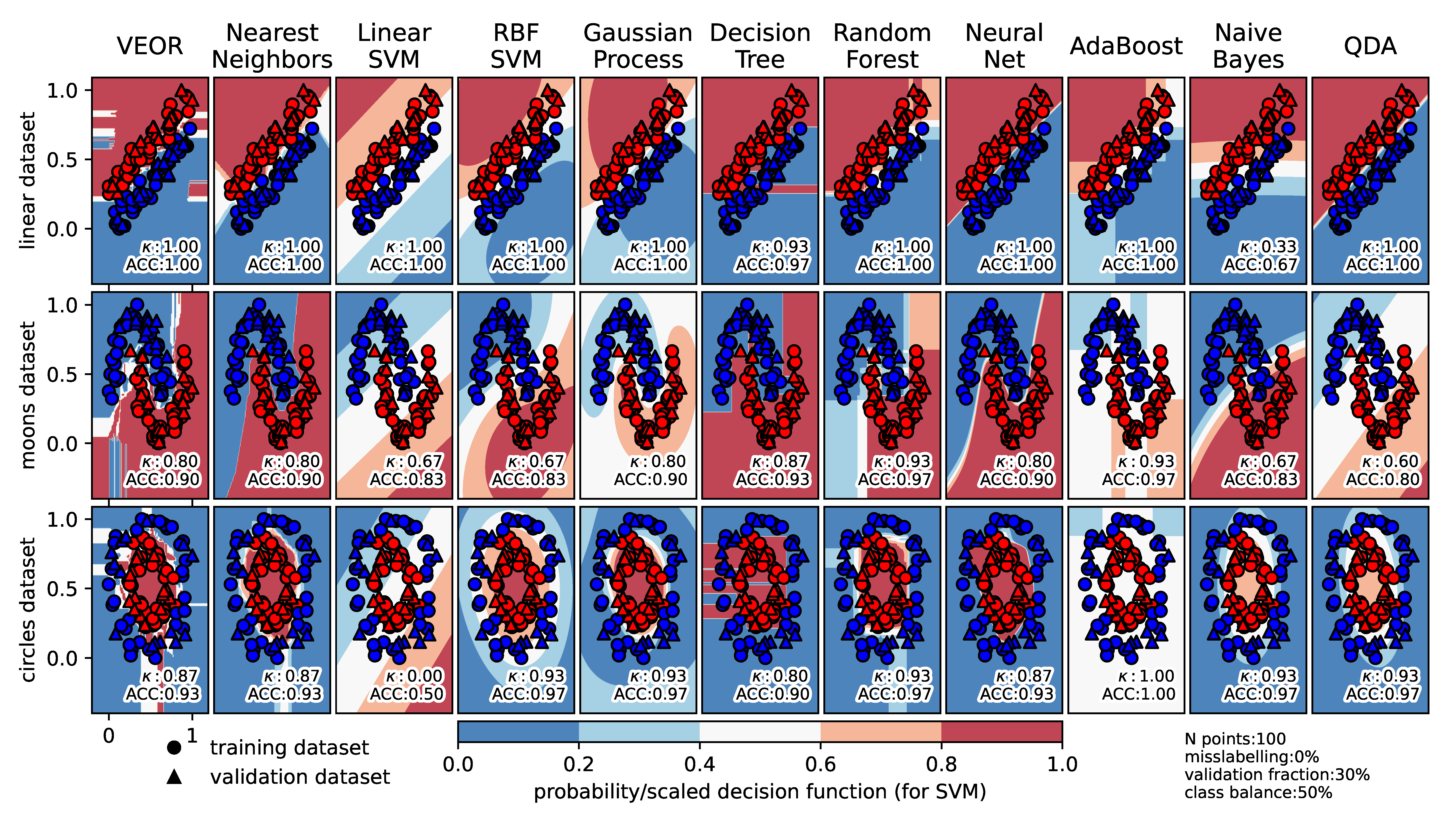
• linear dataset—adapted from the “classifier comparison” script with a linear boundary between groups;
• moons dataset—adapted from the routine “make_moons” from the “sklearn.datasets” module with a non-linear boundary between groups;
• circles dataset—adapted from the routine “make_circles” from the “sklearn.datasets” module with one group forming a ring surrounding another.

For the generation of the 7D case, the “make_classification” routine from the “sklearn.datasets” module was used with the following settings: seven features, three informative features, two redundant features, two irrelevant features, one cluster per class and two classes (binary labeling). The informative features consist of Gaussian clusters each located around the vertices of a hypercube. For each cluster, informative features are drawn independently from N(0, 1) and then randomly linearly combined within each cluster in order to add covariance. The clusters are then placed on the vertices of the hypercube. Redundant features are random linear combinations of the informative features and irrelevant features are merely random samples from the univariate “normal” (Gaussian) distribution. The “make_classification” routine was adapted from [89], where it was used to generate the non-linear “Madelon” dataset used during the Neural Information Processing Systems (NIPS) workshop on feature extraction in 2003. The parameters describing the synthetic datasets are given in

Table 2. Parameters describing synthetic datasets used for the evaluation of selected classifiers.

number of features	2, 7
number of samples	100, 250, 500, 1000
fraction of mislabeled samples (in %)	10, 20, 30
class imbalance (in %)	30/70, 40/60, 50/50

.

5.2. Real Case Datasets

The real case datasets were composed of spectral measurements from the MODIS sensor mounted aboard the AQUA satellite, which were spatially and temporally collocated with the reference cloud mask originating from the Cloud-Aerosol Lidar with Orthogonal Polarization (CALIOP) lidar data acquired by the CALIPSO satellite, as well as the Cloud Profiling Radar (CPR) data acquired by the CloudSat satellite. The AQUA, CALIPSO and CloudSat platforms followed each other closely as part of the A-Train satellite constellation, crossing the equator in an ascending (northbound) direction at approximately 1:30 p.m. local solar time. CloudSat and CALIPSO lagged AQUA by 1 to 2 min and were separated from each other by 10 to 15 s [90]. This allowed for constant spatio-temporal collocations of AQUA’s MODIS measurements with CALIPSO’s CALIOP and CloudSat’s 94 GHz CPR vertical profiles in order to jointly analyze the rapidly changing cloud cover. In this respect, the 2B-GEOPROF-LIDAR product version R05 [90] used in this study includes a number of hydrometeor layers in the vertical column of the CloudSat profile. To separate cloud layers, at least 960 m of hydrometeor free space, as defined by either radar or lidar, must be present. The cloud layers detected by the lidar are computed from the 5 km horizontally averaged Vertical Feature Mask product featuring a native resolution of 333 m. The horizontally averaged product was found to be in best agreement with the MODIS AQUA (MYD35) cloud mask product [90]. Within this study, the reference binary cloud mask used for the training and validation of selected classifiers was generated assuming cloud cover whenever at least one cloud layer was detected either by the CALIOP or CPR instruments.

Along with the 2B-GEOPROF-LIDAR, the MODIS-AUX product [91] is generated, which consists of the Collection 6 AQUA MODIS products that overlap and surround each CPR footprint, namely (1) radiance (MYD02_1KM_L1B product), (2) cloud mask (MYD35_L2 product) and (3) geodetic 1-kilometer resolution latitude and longitude (MYD03). Within the MODIS-AUX product, all MODIS datasets are collocated with the CPR ray using the great-circle nearest neighbor scheme, forming a 3-pixel across-track by 5-pixel along-track spatial subset overlapping each CPR footprint. The maximum allowed collocation distance between a MODIS 1 km pixel and a CPR footprint was set to 0.95 km. As the A-Train constellation satellites follow each other along very similar orbits, most of the collocations are close to the nadir view (mean MODIS satellite zenith angle 15.15° +/− 2.84°). Consequently, the dataset used to train classifiers featured very little angular variability across-track and, in this respect, it was not representative.

Within the presented study, the 2B-GEOPROF-LIDAR and the MODIS-AUX products were further matched by selecting a pixel from the 3-pixel across-track by 5-pixel along-track spatial subset of MODIS products with the smallest distance to the corresponding CPR footprint. Spectral reflectances, brightness temperatures and Sun/sensor geometries derived from the embedded MYD02_1KM_L1B product were used as explanatory variables for the training of selected classifiers and the retrieval of classifications. All explanatory variables were standardized (centered around the mean value with a unit standard deviation) in order to improve the reliability of distance computation required by some classifiers (e.g., KNN, SVM). For the sake of comparison, the MODIS cloud mask was also derived from the embedded MYD35 product and transformed to a binary mask assuming that “confident clear” and “probably clear” pixels are cloud-free whereas “confident cloudy” and “probably cloudy” pixels are filled with clouds. The 2B-GEOPROF-LIDAR and the MODIS-AUX products were split into two independent, temporally decoupled validation and training datasets acquired in 2006 and in 2007, respectively. The analyzed time period was selected due to the earliest possible joint operation time of the AQUA (launched in 2002), CALIPSO (launched in 2006) and CloudSat (launched together with CALIPSO) satellites. At that time, the instruments had experienced very small degradations apart from the MODIS AQUA 1.6 $\mathsf{\mu }$m channel. The full list of spectral and ancillary features used by the classifiers is presented in

Table 3. Spectral and angular features used for cloud discrimination over water surfaces using MODIS imagery.

Abbreviation	Full Name
B1_645nm	Band 1 reflectance at 645 nm
B2_858nm	Band 2 reflectance at 858 nm
B3_469nm	Band 3 reflectance at 469 nm
B4_555nm	Band 4 reflectance at 555 nm
B5_1240nm	Band 5 reflectance at 1.240 $\mathsf{\mu }$m
B7_2130nm	Band 7 reflectance at 2.130 $\mathsf{\mu }$m
B17_905nm	Band 17 reflectance at 905 nm
B18_936nm	Band 18 reflectance at 936 nm
B19_940nm	Band 19 reflectance at 940 nm
B26_1375nm	Band 26 reflectance at 1.375 $\mathsf{\mu }$m
B20_3750nm	Band 20 brightness temperature at 3.750 $\mathsf{\mu }$m
B27_6715nm	Band 27 brightness temperature at 6.715 $\mathsf{\mu }$m
B28_7325nm	Band 28 brightness temperature at 7.325 $\mathsf{\mu }$m
B29_8550nm	Band 29 brightness temperature at 8.550 $\mathsf{\mu }$m
B30_9730nm	Band 30 brightness temperature at 9.730 $\mathsf{\mu }$m
B31_11030nm	Band 31 brightness temperature at 11.030 $\mathsf{\mu }$m
B32_12020nm	Band 32 brightness temperature at 12.020 $\mathsf{\mu }$m
B33_13335nm	Band 33 brightness temperature at 13.335 $\mathsf{\mu }$m
B34_13635nm	Band 34 brightness temperature at 13.635 $\mathsf{\mu }$m
B35_13935nm	Band 35 brightness temperature at 13.935 $\mathsf{\mu }$m
B36_14235nm	Band 36 brightness temperature at 14.235 $\mathsf{\mu }$m
B1_645nm_B2_858nm_ratio	Reflectance ratio between Bands 1 and 2
B31_11030nm_B20_3750nm_diff	Brightness temperature difference between Bands 31 and 20
B32_12020nm_B20_3750nm_diff	Brightness temperature difference between Bands 32 and 20
B31_11030nm_B32_12020nm_diff	Brightness temperature difference between Bands 31 and 32
B28_7325nm_B31_11030nm_diff	Brightness temperature difference between Bands 28 and 31
B29_8550nm_B31_11030nm_diff	Brightness temperature difference between Bands 29 and 31
B29_8550nm_B28_7325nm_diff	Brightness temperature difference between Bands 29 and 28
sunz	Sun zenith angle
satz	Satellite zenith angle
suna	Sun azimuth angle
sata	Satellite azimuth angle
razi	Relative azimuth angle
scat	Scattering angle
NDVI	Normalized Difference Vegetation Index $\mathrm{NDVI}=\frac{\mathrm{B}2\_858\mathrm{nm}-\mathrm{B}1\_645\mathrm{nm}}{\mathrm{B}2\_858\mathrm{nm}+\mathrm{B}1\_645\mathrm{nm}}$

.

The MODIS collocations with CALIOP and CPR were divided into two real cases. The first simple one consisted of daytime data (Sun zenith angle < 85°) over water, away from sun glint areas and excluding polar regions (60°–90° latitudes). The second, more difficult case consisted of daytime data (Sun zenith angle < 85°) over ice/snow. Information about sun glint areas as well as the land/water and snow masks was extracted from the MYD35 product. Each real case dataset was randomly subsampled into 100,000 training samples and 30,000 validation (hold-out) samples.

5.3. Optimization of Classifiers: Forward Feature Selection and Hyper-Parameter Tuning

The classifiers implemented within the scikit-learn library come within a set of default hyper-parameters that should perform well for a wide range of datasets. Nevertheless, this flexibility comes at the price of suboptimal accuracy, which can be further improved by the tuning of hyper-parameters. In this respect, the scikit-learn library version 0.24.2 offers a suite of useful routines, amongst which the HalvingGridSearchCV routine from the sklearn.model_selection module was used within this study. This routine starts by evaluating all combinations of hyper-parameters with a small amount of resources and iteratively selects the best ones, using more and more resources. The term “resources” typically denotes a number of training samples, but it can also be an arbitrary numeric parameter such as a number of trees in a random forest. The optimal combination of hyper-parameters maximizes some classification quality metric (Cohen’s kappa score in this study), which is derived internally by the HalvingGridSearchCV routine, which divides the input samples into the training and held-out samples. It has to be emphasized that the input samples used for the forward feature selection and hyper-parameter tuning consisted of training datasets generated within the experiments with the 2D datasets and MODIS data. The optimal set of hyper-parameters varies for different combinations of input features. Therefore, feature selection was performed, prior to the hyper-parameter tuning, by means of the SequentialFeatureSelector routine from the sklearn.feature_selection module. This routine performs forward feature selection using 5-fold cross-validation, which maximizes some classification quality metric (Cohen’s kappa score in this study). The feature selection procedure was performed only for the real case datasets (summary of the selected features is given in Appendix A). Within the experiments with synthetic 7D datasets with redundant and irrelevant features, the feature selection was not performed on purpose, in order to evaluate the ability of the classifiers to deal with such situations. On the contrary, the hyper-parameter tuning was always performed—separately for every classification process.

5.4. Evaluation of Classifiers

The selected classifiers were assessed in the same consistent way across experiments, using accuracy (ACC) and Cohen’s kappa ($\kappa$) scores to measure the agreement between classified and reference data. The ACC score, defined as the fraction of correctly labeled samples, is widely used; however, it is difficult to interpret for imbalanced datasets (see Section 2.3). In such a case, Cohen’s kappa score [60] is more robust as it takes into account the possibility of agreement occurring by chance. Its values range from −1 to 1, where 1 is perfect agreement between predicted and reference labels, 0 denotes (dis)agreement that would be obtained by a completely random classifier, whereas negative values denote (dis)agreement that is worse than random. The formula for Cohen’s kappa score is given by Equation (3).

$$\kappa =\frac{P_o-P_e}{1-P_e}$$

(3)

where:

$P_o$—empirical probability of agreement between predicted and reference labels (same as ACC);

$P_e$—hypothetical probability of agreement between randomly assigned and reference labels.

The randomly generated synthetic datasets introduced stochastic variations of derived classification quality metrics. Therefore, the experiments with the synthetic datasets were repeated 30 times for each combination of three variables: number of samples, class imbalance and noise level. In the case of the daytime cloud detection over water surfaces using the MODIS/CALIPSO/CPR collocations, the analysis was run once with the training dataset collected in 2007 and the validation dataset from 2006.

Ultimately, the numerical performance of the classifiers in terms of the execution times of the training and retrieval processes separately was investigated. The machine used for this analysis was based on the AMD EPYC 7401 24-Core Processor with 256 GB RAM, running the Ubuntu version 18.04.5 operating system with a Python 3.9.6 environment containing the NumPy version 1.21.1, Scipy version 1.7.14. and scikit-learn version 0.24.2 libraries. For the sake of comparability, the multicore/hyper-threading support for the selected classifiers (including the VEOR) was deactivated in order to measure the single-core numerical performance. For this analysis, the linear synthetic dataset with an increasing number of samples (${10}^2$, ${10}^3$, ${10}^4$, ${10}^5$, ${10}^6$) was used, and each analysis was repeated five times to generate mean execution times. In the case of the Gaussian process classifier, training of more than ${10}^4$ samples was computationally too expensive and the execution times for those datasets were not measured.

6. Results

6.1. Classification of Synthetic 2D Datasets

Initially, the evaluation of the selected algorithms involved a binary classification of three types of randomly generated synthetic datasets composed of two features separated by linear, non-linear and circular borders (see rows in Figure 4), which were further grouped according to a classification in terms of difficulty: easy, moderate and difficult (see Section 5.1). An exemplary experiment with an easy dataset is presented in Figure 4, where blue points are labeled with 0 and red with 1. Circles denote training points and triangles denote validation points, which were split according to a 70%/30% proportion, respectively. In the background, the classification probability or decision function, scaled to a 0–1 range for SVM, is presented for every sample within the 2D grid. The accuracy (ACC) and kappa ($\kappa$) values are also reported, although they are not conclusive due to the randomness of synthetic datasets, which introduces great variability between algorithms, especially for datasets with a low number of samples (see standard deviation whiskers in Figure 5). Nevertheless, some interesting conclusions can be drawn regarding the inability of some classifiers to fit the samples. In this respect, it is not surprising that linear SVM is unable to fit datasets with non-linear and circular borders. However, it is more interesting that the Naive Bayes classifier is unable to fit the simplest linear dataset, most likely because, in this case, the feature independence assumption is strongly violated. Likewise, for the moons dataset, the RBF SVM, Naive Bayes and QDA classifiers performed poorly, but the same methods performed well for the circles dataset (presumably the most difficult to classify). The classification probability/scaled decision function presented in the background of Figure 4 reveals interesting patterns. Algorithms based on data partitioning, such as VEOR, decision tree, random forest and AdaBoost, produced jagged results, whereas algorithms that model/fit the probability field (i.e., SVM, Gaussian process, neural net, Naive Bayes, QDA) produce smoother results. A quantitative analysis of the classification results for the linear, moons and circles datasets, grouped together according to classification difficulty (see Section 5.1), is presented in Figure 5. The general pattern apparent from this analysis reveals that the number of samples is directly proportional to the classification accuracy and inversely proportional to the variability of derived classification metrics. This is particularly noticeable for the VEOR algorithm, where a small training dataset leads to a low number of samples within the percentile grid and consequently to variable classification probability estimates that are difficult to reconstruct by the KNN weighted average. The same applies to noisy training datasets, where the reconstruction of probability is challenging even for a large number of nearest neighbors, resulting in significant probability smoothing. In such a case, the algorithms that model/fit to the classification probability field, such as RBF SVM, Gaussian process and neural net, perform best. On the contrary, the linear SVM, decision tree and Naive Bayes classifiers seem to be the least accurate and they do not “learn” much from the larger training datasets (see the median line marked on the boxes in Figure 5). This implies that if the assumptions behind these algorithms are violated (e.g., linearity, feature independence), they will not improve the classification skills given more training samples. Ultimately, it has to be emphasized that the experiment with the 2D datasets was an idealized case where only two important/meaningful features were used. In reality, the classification is usually based on more features, including some irrelevant or redundant ones. This aspect was investigated in the experiment with the 7D dataset, described in the next subsection.

6.2. Classification of Synthetic 7D Datasets

The experiment with the synthetic 7D datasets was performed analogously to the evaluation of the 2D datasets, apart from the feature vector, which consisted of three informative/meaningful features, two redundant features and two irrelevant features. No feature selection was applied during the optimization of classifiers within this experiment in order to test the sensitivity of each method to irrelevant and redundant features. Evaluation of the classifiers’ performance used for the 7D dataset (Figure 6) revealed a similar pattern to the experiment with the 2D datasets, except for the linear SVM and Naive Bayes classifiers, which performed well this time. The least accurate was the decision tree classifier, which is very sensitive to the irrelevant and noisy information that forms spurious branches within a tree structure. This in turn deteriorates the ability of a classifier to generalize to new/unseen cases. Thus, a tree pruning procedure should be applied, which was optimized within this study by means of the ccp_alpha hyper-parameter that controls the Minimal Cost-Complexity Pruning method [43]. Surprisingly, for a small number of points, the random forest classifier performed better than the AdaBoost method, which is supposed to incorporate the decision tree classifications more efficiently than the former algorithm. Across selected classifiers, the VEOR algorithm performed well for the easy and moderate datasets, while, for the difficult datasets, the classification accuracy was slightly worse than other methods.

6.3. Cloud Detection Using Daytime MODIS Spectral Measurements and a Reference Cloud Mask Derived from Combined CALIOP and CPR Data

6.3.1. Cloud Detection over Water Surfaces

Within the real case experiment involving cloud discrimination using MODIS satellite spectral measurements (Figure 7), the reference quality metrics (ACC = 0.879, $\kappa$ = 0.723) for the selected classifiers were derived from the Collection 6 AQUA MODIS cloud mask product (MYD35). In this respect, it has to be emphasized that the MYD35 product is globally applicable for all satellite zenith angles, whereas the classifiers selected are applicable close to the satellite nadir (due to an unrepresentative training dataset). Despite this fact, the decision tree classifier produced inferior results to the MYD35 product (ACC = 0.840, $\kappa$ = 0.627), whereas all other methods with optimized hyper-parameters generated very similar and accurate classifications. As compared to the VEOR algorithm (ACC = 0.888, $\kappa$ = 0.748), the Naive Bayes (ACC = 0.880, $\kappa$ = 0.734), Gaussian process (ACC = 0.882, $\kappa$ = 0.736), QDA (ACC = 0.883, $\kappa$ = 0.736), nearest neighbor (ACC = 0.884, $\kappa$ = 0.738), linear SVM (ACC = 0.885, $\kappa$ = 0.739) and RBF SVM (ACC = 0.886, $\kappa$ = 0.745) classifiers were slightly less accurate, while the random forest (ACC = 0.889, $\kappa$ = 0.747), neural net (ACC = 0.890, $\kappa$ = 0.752) and AdaBoost (ACC = 0.891, $\kappa$ = 0.753) classifiers were slightly more accurate. It could be noticed that many classifiers discriminated cloud cover over water surfaces with almost the same classification quality metrics. This may indicate that several methods reached almost maximum classification accuracy given the radiometric sensitivity of the MODIS instrument and the collocation inaccuracies with the CALIOP and CPR sensors.

Regardless of the very similar classification results, the forward feature selection procedure applied to each classifier resulted in different optimal combinations of input features over water surfaces (see Appendix A). In this respect, the VEOR algorithm selected four optimal features ordered according to decreasing importance: B18_936nm, B32_12020nm, sunz, B30_9730nm (for abbreviations, see Table 3). The first two features (the most important) were also selected by the nearest neighbor, neural net, decision tree and random forest classifiers, while linear SVM, Naive Bayes and QDA did not select even one of them. Other features that were often selected were: B29_8550nm_B31_11030nm_diff (6 times), B29_8550nm_B31_11030nm_diff (3 times), B29_8550nm_B31_11030nm_diff (3 times), NDVI (3 times). All of the algorithms apart from the linear SVM required some angular feature, but the type of this information varied significantly. The Sun zenith angle was required only by the VEOR algorithm. The Sun azimuth angle was optimal for the nearest neighbor, decision tree and Naive Bayes classifiers. The scattering angle was selected by the neural network, random forest, AdaBoost, Naive Bayes and QDA algorithms, while the relative azimuth angle was required by the RBF SVM and Gaussian process classifiers. The satellite zenith angle was not selected by any method because collocations of the CALIPSO and CPR profiles with the AQUA MODIS radiometer were only available close to the satellite nadir. The inconsistency in the selected angular features is not easily explainable as it is a combination of physics and data sampling. Based on the VEOR output, the angular information itself is a weak classification feature for cloud discrimination and it slightly improves the overall accuracy over water surfaces close to the satellite nadir. Thus, in the case of the stochastic classifiers, different features (including angular ones) might be selected between consecutive algorithm runs with the same input data.

Cloud discrimination over water surfaces during daytime is a fairly simple classification task. Therefore, to fully evaluate the performance of the selected classifiers, an analogous experiment over snow/ice surfaces was performed (see next subsection).

6.3.2. Cloud Detection over Ice/Snow Surfaces

Cloud discrimination over ice/snow surfaces during daytime is more challenging than over water surfaces due to the low optical and thermal contrasts between the surface and clouds (see Section 2.2). This is particularly apparent in the case of the MYD35 product (Figure 8), which, over ice/snow, is 21% less accurate than over water (ACC = 0.671 vs. ACC = 0.881), and the Cohens’ kappa is 56% lower (ACC = 0.727, $\kappa$ = 0.317). Amongst the selected classifiers, only the Naive Bayes method produced worse results than the MYD35 product (ACC = 0.659, $\kappa$ = 0.296). As compared to the VEOR algorithm (ACC = 0.809, $\kappa$ = 0.611), the QDA (ACC = 0.742, $\kappa$ = 0.467) and decision tree (ACC = 0.764, $\kappa$ = 0.526) methods were less accurate, the nearest neighbor (ACC = 0.809, $\kappa$ = 0.614) and linear SVM (ACC = 0.808, $\kappa$ = 0.613) classifiers were equally accurate, while the AdaBoost (ACC = 0.816, $\kappa$ = 0.629), random forest (ACC = 0.818, $\kappa$ = 0.632), Gaussian process (ACC = 0.822, $\kappa$ = 0.639), RBF SVM (ACC = 0.886, $\kappa$ = 0.745) and neural net (ACC = 0.890, $\kappa$ = 0.752) algorithms were more accurate. Regarding the optimal feature combination for cloud discrimination over ice/snow (see Appendix A), the internal VEOR feature selection procedure selected the following features (ordered by decreasing significance): B7_2130nm, B18_936nm, B26_1375nm, B3_469nm. In this respect, MODIS reflectance at 2130 nm was selected by all of the classifiers apart from the Naive Bayes classifier, while the reflectance at 936 nm was selected by the nearest neighbor, neural network, RBF SVM, random forest and AdaBoost methods. Other features that were often selected were: B29_8550nm_B28_7325nm_diff (5 times), B27_6715nm (4 times), B32_12020nm (3 times), B28_7325nm (3 times). As opposed to the cloud discrimination over water surfaces, only the linear SVM classifier required angular information (i.e., Sun zenith angle) to discriminate cloud cover over ice/snow surfaces.

6.4. Numerical Performance Evaluation

The evaluation of numerical performance revealed great differences between the single-core computational requirements of the selected classifiers. The most demanding from the perspective of classifier training is the Gaussian process algorithm, which was not able to be applied for 2D datasets with more than ${10}^5$ samples; thus, only results for ${10}^2$, ${10}^3$, ${10}^4$ are reported in Figure 9. However, the retrieval time for this classifier is in the order of tens of seconds for a dataset with ${10}^6$ samples (Figure 10), which might be applicable to moderate-resolution imagery. Another numerically expensive algorithm is the RBF SVM, which takes hours for training and tens of minutes to classify a dataset with ${10}^6$ samples. Thus, this method might be applicable for the classification of a single image. On the contrary, the linear SVM classifier is numerically robust, with a retrieval time a few orders of magnitude faster than other techniques. Interestingly, the RBF SVM routine can be executed with a linear kernel (instead of the RBF kernel), which is supposed to be conceptually the same as the linear SVM method. However, due to the different libraries used by these two routines (liblinear vs. libsvm), the reduction in processing time is from hours to seconds for algorithm training, and from minutes to milliseconds for classification retrieval. Thus, it has to be emphasized again that the presented results depend heavily on scikit-learn implementation, and for other machine learning libraries, the numerical performance of selected classifiers may differ significantly. The least numerically demanding methods for both training and retrieval are the Naive Bayes and QDA algorithms. Other methods, such as random forest, neural net and AdaBoost, which provided accurate classification results (see Figure 5, Figure 6 and Figure 7), are also numerically efficient, which might be the reason for their popularity amongst the machine learning community.

The processing time for the VEOR classifier scales efficiently with the number of samples due to the utilization of the fast cKDTree method, which performs worse than a “brute-force” search for a small number of samples but is very robust for large datasets. The largest improvement in processing time for the VEOR algorithm over the nearest neighbor classifier (which also involves searching) is noticeable for classification retrieval. This is due to the utilization of a fast binary search algorithm applied over a vector with sorted ID. Consequently, almost two orders of magnitude of speed improvement are gained over the cKDTree method, which additionally requires the computation of distance metrics in multiple dimensions. Finally, it has to be stated that the reported relationships between the processing times of the selected classifiers may change with other datasets featuring more dimensions, more noise or different class separability. Thus, the presented results are more qualitative than quantitative and could provide a general idea about the numerical performance of the selected classifiers implemented in the scikit-learn library version 0.24.2.

7. Discussion

The experiments with the classification of synthetic and satellite datasets revealed that the VEOR algorithm provides similar or better classification results compared with other widely used machine learning algorithms with fine-tuned hyper-parameters and optimized input features. In this respect, it performed among the top 3–5 most accurate algorithms for synthetic datasets with low and moderate levels of noise and class imbalance, as well as for cloud detection using MODIS/CALIOP/CPR collocations. For small, noisy (30% of mislabeling) and imbalanced (30%/70%) datasets, the VEOR provided moderate results comparable to the random forest classifier. This is due to the fact that a significantly disturbed classification probability field is difficult to reconstruct by means of a simple inverse distance weighted average, and thus has to be modeled. Therefore, the classifiers that involve more advanced modeling approaches, such as SVM or Gaussian process, perform better for such datasets but at the price of large computational costs. Nevertheless, classification of an extensive volume of remote sensing data requires a method that is both numerically efficient and accurate. Such a combination is reached by the neural network classifier, which provides accurate classification results, but its internal configuration is difficult to interpret. In this respect, the VEOR method ranks single features and combinations of features according to Cohen’s kappa score. This greatly facilitates the understanding of the feature selection process.

Conceptually simple methods such as nearest neighbor, Naive Bayes or QDA do not fit well with all datasets, especially with multispectral MODIS measurements over ice/snow surfaces. Interestingly, for some difficult synthetic datasets, these methods perform well in comparison to the most robust classifiers. This may indicate that if some assumptions behind such methods are met (e.g., Gaussian distribution describing each class and/or linear separability of classes), then they are able to provide accurate classification results with great numerical efficiency. Another type of classifier is the so-called “weak learners”, such as the decision tree algorithm, which generally do not feature good classification skills (see Figure 5, Figure 6, Figure 7 and Figure 8) but are extremely fast and simple to apply. Therefore, they can be executed multiple or hundreds of times with different settings and their stochastic results can be further post-processed to derive an accurate ensemble classifier such as the random forest or AdaBoost. The latter algorithms were found to be robust especially for the classification of multispectral MODIS data and synthetic datasets with a low level of noise and small class imbalance. The reiteration of a stochastic classifier several times with the same input data increases the representability of the classification results, as some initial settings within an algorithm optimization are set by a random guess. Consequently, without repetition, the stochastic classifiers (e.g., decision tree) may provide significantly different results for the same input data. Another source of algorithm instability may be caused by a convergence problem when an iterative algorithm optimization procedure fails due to an unrealistic assumption (e.g., linearity in the case of the linear SVM) or a small number of iterations. Apart from the classifier itself, an additional source of variability in the performed experiments originates from the stochastic wrapper procedures to optimize the hyper-parameters (HalvingGridSearchCV—scikit-learn library routine) and to select the most optimal features (SequentialFeatureSelector—scikit-learn library routine). Therefore, it has to be noted that the presented evaluation results and ranking of the classifiers are prone to small changes related to the random state/random seed of the pseudo-random number generator embedded within the scikit-learn library.

Application of a classifier to large EO datasets requires numerical efficiency, especially concerning the retrieval processing time. In this respect, the classification of a 2D dataset composed of ${10}^6$ samples took longest for the RBF SVM method (1668 s), while, for the linear SVM, it took the shortest time (0.002 s). The main reason for this drastic reduction in processing time originates from the different libraries, and not from algorithm differences per se (retrieval time for the SVM routine with linear instead of an RBF kernel also took several minutes). This implies that before rejecting a classifier due to numerical inefficiency, it is advisable to test its different implementations (if possible). The VEOR implementation in the Python programming language appeared to be numerically robust due to the implementation of the fast cKDTree algorithm for finding the nearest cells within the percentile grid and a binary search algorithm to extract the classification probabilities from the LUV. Thus, the VEOR retrieval is one of the fastest amongst the selected classifiers and therefore can be applied to extremely large EO datasets. On the contrary, the scikit-learn implementation of the RBF SVM and Gaussian process classifiers is not suitable for the processing of large datasets. The analyses performed revealed that there is no single classifier that would outperform all the other methods for all analyzed datasets. However, a few algorithms performed well in almost all cases. In this respect, the neural network method accurately classified synthetic datasets, which were significantly disturbed by noise and class imbalance. It also discriminated cloud cover over water surfaces using MODIS spectral measurements well, with accuracy comparable to the random forest and AdaBoost methods, which provided the best results in this case (~1% better than the MYD35 product). However, more noticeable differences were revealed by the experiment with a daytime cloud discrimination over ice/snow, where the neural network classifier performed the best—17% more accurate than the MYD35 product and 0.5% better than the second best RBF SVM classifier (Figure 8). Almost all classifiers, apart from the Naive Bayes, outperformed the MYD35 collection 6 product over snow, which implies that there is still great potential for improvement of the MODIS cloud mask product. However, it has to be again strongly emphasized that the acquired results refer only to low satellite zenith angles as the AQUA MODIS collocations with the CALIOP and CPR profiles are only available close to the satellite nadir. This is also a reason that the satellite zenith angle was not selected either by the VEOR or by the SequentialFeatureSelector routine applied to other classifiers (see Appendix A). In this respect, there is interesting inconsistency in combinations of the MODIS spectral and angular features optimized for every classifier, especially for the relatively easy experiment with the daytime cloud discrimination over water surfaces, where almost all of the classifiers performed almost equally well. This may indicate that several combinations of spectral and angular features may lead to the same optimal results. On the other hand, within a more difficult experiment with the daytime cloud discrimination over ice/snow, the performance of the evaluated classifiers varied more significantly along with the combinations of selected features. This may imply that the feature selection procedure may produce incorrect results if the classification skills of the classifier being optimized are low (see results of the Naive Bayes classifier in Figure 8 and the corresponding optimal feature combination listed in Appendix A). Nevertheless, the experiments conducted within this study and the extensive literature [47,48] lead to the conclusion that the feature selection significantly improves the classification results.

Ultimately, it has to be stated that the VEOR classifier performed well for datasets with many samples, including the experiment with MODIS data, where it proved that the combination of four features allows for more accurate (by ~1% over water surfaces and by ~14% over ice/snow) cloud discrimination than the MYD35 product. The feature selection procedure implemented in VEOR reports Cohen’s kappa coefficient for every analyzed combination of features. This is computationally feasible due to the simple reconstruction of the classification probability field by means of the weighted inverse distance K-nearest neighbor average. Nevertheless, such a solution is not accurate for small datasets, especially with significant noise and class imbalance. However, the premise for VEOR development was the derivation of an accurate probabilistic classification for large EO datasets requiring some methodological simplifications. Several experiments conducted within this study have proven that the VEOR classifier is an interesting alternative to common machine learning techniques.

8. Conclusions

The main objective of this work was to evaluate the performance of the novel self-optimizing probabilistic Vectorized Earth Observation Retrieval (VEOR) classifier with respect to common machine learning algorithms with fine-tuned hyper-parameters and optimized input features. This was achieved within a series of experiments with synthetic datasets, as well as with daytime cloud discrimination using AQUA MODIS spectral measurements and a reference cloud mask derived from combined CALIOP lidar and CPR radar data. The classification results proved that the VEOR method is able to accurately classify large datasets commonly occurring within various Earth Observation (EO) disciplines. However, it is not suitable for small and noisy datasets due to the imprecise reconstruction of the multidimensional classification probability field by means of a weighted inverse distance average when the number of samples is limited. Nevertheless, comparison with other classifiers revealed that the VEOR algorithm is within the 3–5 most robust techniques for large (i.e., >=1000 samples) synthetic datasets with low or moderate levels of noise and class imbalance. More importantly, it performed well for the daytime cloud masking over water surfaces using MODIS spectral measurements (ACC = 0.888, $\kappa$ = 0.748), where it was better than the reference MODIS cloud mask collection 6 product (ACC = 0.881, $\kappa$ = 0.727), but slightly worse than the random forest (ACC = 0.889, $\kappa$ = 0.747), neural net (ACC = 0.890, $\kappa$ = 0.752) and AdaBoost (ACC = 0.891, $\kappa$ = 0.753) classifiers. An analogous experiment over ice/snow revealed that the VEOR algorithm is again more accurate (ACC = 0.809, $\kappa$ = 0.611) than the MODIS cloud mask (ACC = 0.671, $\kappa$ = 0.317) and less accurate than the AdaBoost (ACC = 0.816, $\kappa$ = 0.629), random forest (ACC = 0.818, $\kappa$ = 0.632), Gaussian process (ACC = 0.822, $\kappa$ = 0.639), RBF SVM (ACC = 0.886, $\kappa$ = 0.745) and neural net (ACC = 0.890, $\kappa$ = 0.752) classifiers. Interestingly, the forward feature selection method applied to each classifier resulted in a wide range of optimal combinations of features. This is particularly surprising for the daytime cloud discrimination over water surfaces, where different combinations of input features led to almost the same results. Within a more difficult experiment with daytime cloud discrimination over ice/snow, the feature selection was not effective for classifiers featuring limited classification skills over ice/snow (i.e., Naive Bayes method). Finally, it has to be emphasized that the acquired results refer only to low satellite zenith angles as the AQUA MODIS collocations with the CALIOP and CPR profiles are only available close to the satellite nadir.

The performed experiments revealed that the decision tree, linear SVM and Naive Bayes produced variable results for the synthetic datasets, provided that some internal assumptions were met or not. The Gaussian process and RBF SVM (based on the libsvm library) classifiers were found to be accurate even for small datasets with a significant noise level. However, their complexity and current implementation within the scikit-learn library do not allow for their application to large EO datasets. Ultimately, the VEOR algorithm features some unique characteristics amongst analyzed classifiers, such as:

• numerically efficient probabilistic classification of large, multidimensional datasets;
• an internal feature selection method that allows the minimal feature subset required for optimal classification results to be identified;
• the ranking of classification skills for analyzed feature combinations according to Cohen’s kappa coefficient;
• intuitive interpretation of derived optimal algorithm settings (including selected features);
• easily expandable LUV whenever new data have to be added to a training dataset.

These characteristics, supported by the analytical results in this study, lead to the final conclusion that the VEOR classifier is an interesting alternative to existing machine learning methods, especially in terms of the classification of large multidimensional EO datasets. Further development of the VEOR algorithm will involve adaptive reconstruction of the multidimensional classification probability field, where the number of nearest neighboring cells K (see Equation (2)) will not be constant for all cells, but it will be further optimized to a specific location within the probability field. Moreover, a more sophisticated inverse distant weighting scheme used within the reconstruction of the multidimensional classification probability field will be proposed. These adaptations should further improve the accuracy of the VEOR classifier and increase its competitiveness with other machine learning algorithms.

References

1. Anderson, J.R. A Land Use and Land Cover Classification System for Use with Remote Sensor Data; US Government Printing Office: Washington, DC, USA, 1976; Volume 964. [Google Scholar]
2. Friedl, M.A.; Sulla-Menashe, D.; Tan, B.; Schneider, A.; Ramankutty, N.; Sibley, A.; Huang, X. MODIS Collection 5 global land cover: Algorithm refinements and characterization of new datasets. Remote Sens. Environ. 2010, 114, 168–182. [Google Scholar] [CrossRef]
3. Hansen, M.C.; Loveland, T.R. A review of large area monitoring of land cover change using Landsat data. Remote Sens. Environ. 2012, 122, 66–74. [Google Scholar] [CrossRef]
4. Inglada, J.; Vincent, A.; Arias, M.; Tardy, B.; Morin, D.; Rodes, I. Operational high resolution land cover map production at the country scale using satellite image time series. Remote Sens. 2017, 9, 95. [Google Scholar] [CrossRef] [Green Version]
5. Talukdar, S.; Singha, P.; Mahato, S.; Pal, S.; Liou, Y.A.; Rahman, A. Land-use land-cover classification by machine learning classifiers for satellite observations—A review. Remote Sens. 2020, 12, 1135. [Google Scholar] [CrossRef] [Green Version]
6. Defourny, P.; Bontemps, S.; Bellemans, N.; Cara, C.; Dedieu, G.; Guzzonato, E.; Hagolle, O.; Inglada, J.; Nicola, L.; Rabaute, T.; et al. Near real-time agriculture monitoring at national scale at parcel resolution: Performance assessment of the Sen2-Agri automated system in various cropping systems around the world. Remote Sens. Environ. 2019, 221, 551–568. [Google Scholar] [CrossRef]
7. Kussul, N.; Lavreniuk, M.; Skakun, S.; Shelestov, A. Deep learning classification of land cover and crop types using remote sensing data. IEEE Geosci. Remote Sens. Lett. 2017, 14, 778–782. [Google Scholar] [CrossRef]
8. Li, R.; Xu, M.; Chen, Z.; Gao, B.; Cai, J.; Shen, F.; He, X.; Zhuang, Y.; Chen, D. Phenology-based classification of crop species and rotation types using fused MODIS and Landsat data: The comparison of a random-forest-based model and a decision-rule-based model. Soil Tillage Res. 2021, 206, 104838. [Google Scholar] [CrossRef]
9. Sonobe, R.; Tani, H.; Wang, X.; Kobayashi, N.; Shimamura, H. Random forest classification of crop type using multi-temporal TerraSAR-X dual-polarimetric data. Remote Sens. Lett. 2014, 5, 157–164. [Google Scholar] [CrossRef] [Green Version]
10. Adam, E.; Mutanga, O.; Rugege, D. Multispectral and hyperspectral remote sensing for identification and mapping of wetland vegetation: A review. Wetl. Ecol. Manag. 2010, 18, 281–296. [Google Scholar] [CrossRef]
11. Bourgeau-Chavez, L.; Kasischke, E.; Brunzell, S.; Mudd, J.; Smith, K.; Frick, A. Analysis of space-borne SAR data for wetland mapping in Virginia riparian ecosystems. Int. J. Remote Sens. 2001, 22, 3665–3687. [Google Scholar] [CrossRef]
12. DeLancey, E.R.; Simms, J.F.; Mahdianpari, M.; Brisco, B.; Mahoney, C.; Kariyeva, J. Comparing deep learning and shallow learning for large-scale wetland classification in Alberta, Canada. Remote Sens. 2020, 12, 2. [Google Scholar] [CrossRef] [Green Version]
13. McCarthy, M.J.; Radabaugh, K.R.; Moyer, R.P.; Muller-Karger, F.E. Enabling efficient, large-scale high-spatial resolution wetland mapping using satellites. Remote Sens. Environ. 2018, 208, 189–201. [Google Scholar] [CrossRef]
14. Carroll, M.L.; Townshend, J.R.; DiMiceli, C.M.; Noojipady, P.; Sohlberg, R.A. A new global raster water mask at 250 m resolution. Int. J. Digit. Earth 2009, 2, 291–308. [Google Scholar] [CrossRef]
15. Donchyts, G.; Baart, F.; Winsemius, H.; Gorelick, N.; Kwadijk, J.; Van De Giesen, N. Earth’s surface water change over the past 30 years. Nat. Clim. Chang. 2016, 6, 810–813. [Google Scholar] [CrossRef]
16. Feng, M.; Sexton, J.O.; Channan, S.; Townshend, J.R. A global, high-resolution (30-m) inland water body dataset for 2000: First results of a topographic–spectral classification algorithm. Int. J. Digit. Earth 2016, 9, 113–133. [Google Scholar] [CrossRef] [Green Version]
17. Wang, G.; Wu, M.; Wei, X.; Song, H. Water identification from high-resolution remote sensing images based on multidimensional densely connected convolutional neural networks. Remote Sens. 2020, 12, 795. [Google Scholar] [CrossRef] [Green Version]
18. Martin, M.; Newman, S.; Aber, J.; Congalton, R. Determining forest species composition using high spectral resolution remote sensing data. Remote Sens. Environ. 1998, 65, 249–254. [Google Scholar] [CrossRef]
19. Hościło, A.; Lewandowska, A. Mapping forest type and tree species on a regional scale using multi-temporal Sentinel-2 data. Remote Sens. 2019, 11, 929. [Google Scholar] [CrossRef] [Green Version]
20. Sheykhmousa, M.; Mahdianpari, M.; Ghanbari, H.; Mohammadimanesh, F.; Ghamisi, P.; Homayouni, S. Support vector machine vs. random forest for remote sensing image classification: A meta-analysis and systematic review. IEEE J. Sel. Top. Appl. Earth Obs. Remote Sens. 2020, 13, 6308–6325. [Google Scholar] [CrossRef]
21. Tang, L.; Shao, G. Drone remote sensing for forestry research and practices. J. For. Res. 2015, 26, 791–797. [Google Scholar] [CrossRef]
22. Hall, D.K.; Riggs, G.A.; Salomonson, V.V. MODIS snow and sea ice products. In Earth Science Satellite Remote Sensing; Springer: Berlin/Heidelberg, Germany, 2006; pp. 154–181. [Google Scholar]
23. Cannistra, A.F.; Shean, D.E.; Cristea, N.C. High-resolution CubeSat imagery and machine learning for detailed snow-covered area. Remote Sens. Environ. 2021, 258, 112399. [Google Scholar] [CrossRef]
24. Schneider, A.; Friedl, M.A.; Potere, D. A new map of global urban extent from MODIS satellite data. Environ. Res. Lett. 2009, 4, 044003. [Google Scholar] [CrossRef] [Green Version]
25. Wang, L.; Li, C.; Ying, Q.; Cheng, X.; Wang, X.; Li, X.; Hu, L.; Liang, L.; Yu, L.; Huang, H.; et al. China’s urban expansion from 1990 to 2010 determined with satellite remote sensing. Chin. Sci. Bull. 2012, 57, 2802–2812. [Google Scholar] [CrossRef] [Green Version]
26. Zhang, Y.; Qin, K.; Bi, Q.; Cui, W.; Li, G. Landscape Patterns and Building Functions for Urban Land-Use Classification from Remote Sensing Images at the Block Level: A Case Study of Wuchang District, Wuhan, China. Remote Sens. 2020, 12, 1831. [Google Scholar] [CrossRef]
27. Heidinger, A.K.; Evan, A.T.; Foster, M.J.; Walther, A. A naive Bayesian cloud-detection scheme derived from CALIPSO and applied within PATMOS-x. J. Appl. Meteorol. Climatol. 2012, 51, 1129–1144. [Google Scholar] [CrossRef]
28. Karlsson, K.G.; Johansson, E.; Devasthale, A. Advancing the uncertainty characterisation of cloud masking in passive satellite imagery: Probabilistic formulations for NOAA AVHRR data. Remote Sens. Environ. 2015, 158, 126–139. [Google Scholar] [CrossRef] [Green Version]
29. Marchant, B.; Platnick, S.; Meyer, K.; Arnold, G.T.; Riedi, J. MODIS Collection 6 shortwave-derived cloud phase classification algorithm and comparisons with CALIOP. Atmos. Meas. Tech. 2016, 9, 1587–1599. [Google Scholar] [CrossRef] [PubMed] [Green Version]
30. Håkansson, N.; Adok, C.; Thoss, A.; Scheirer, R.; Hörnquist, S. Neural network cloud top pressure and height for MODIS. Atmos. Meas. Tech. 2018, 11, 3177–3196. [Google Scholar] [CrossRef] [Green Version]
31. Wang, C.; Platnick, S.; Meyer, K.; Zhang, Z.; Zhou, Y. A machine-learning-based cloud detection and thermodynamic-phase classification algorithm using passive spectral observations. Atmos. Meas. Tech. 2020, 13, 2257–2277. [Google Scholar] [CrossRef]
32. Lu, D.; Weng, Q. A survey of image classification methods and techniques for improving classification performance. Int. J. Remote Sens. 2007, 28, 823–870. [Google Scholar] [CrossRef]
33. Mantero, P.; Moser, G.; Serpico, S.B. Partially supervised classification of remote sensing images through SVM-based probability density estimation. IEEE Trans. Geosci. Remote Sens. 2005, 43, 559–570. [Google Scholar] [CrossRef]
34. Pelletier, C.; Valero, S.; Inglada, J.; Champion, N.; Marais Sicre, C.; Dedieu, G. Effect of training class label noise on classification performances for land cover mapping with satellite image time series. Remote Sens. 2017, 9, 173. [Google Scholar] [CrossRef] [Green Version]
35. Musial, J.P.; Verstraete, M.M.; Gobron, N. Comparing the effectiveness of recent algorithms to fill and smooth incomplete and noisy time series. Atmos. Chem. Phys. 2011, 11, 7905–7923. [Google Scholar] [CrossRef] [Green Version]
36. Millard, K.; Richardson, M. On the importance of training data sample selection in random forest image classification: A case study in peatland ecosystem mapping. Remote Sens. 2015, 7, 8489–8515. [Google Scholar] [CrossRef] [Green Version]
37. Langley, P.; Sage, S. Induction of selective Bayesian classifiers. In Uncertainty Proceedings 1994; Elsevier: Amsterdam, The Netherlands, 1994; pp. 399–406. [Google Scholar]
38. Foody, G.M. The continuum of classification fuzziness in thematic mapping. Photogramm. Eng. Remote Sens. 1999, 65, 443–452. [Google Scholar]
39. Benz, U.C.; Hofmann, P.; Willhauck, G.; Lingenfelder, I.; Heynen, M. Multi-resolution, object-oriented fuzzy analysis of remote sensing data for GIS-ready information. ISPRS J. Photogramm. Remote Sens. 2004, 58, 239–258. [Google Scholar] [CrossRef]
40. Li, Y.; Lu, T.; Li, S. Subpixel-pixel-superpixel-based multiview active learning for hyperspectral images classification. IEEE Trans. Geosci. Remote Sens. 2020, 58, 4976–4988. [Google Scholar] [CrossRef]
41. Sun, B.; Chen, S.; Wang, J.; Chen, H. A robust multi-class AdaBoost algorithm for mislabeled noisy data. Knowl.-Based Syst. 2016, 102, 87–102. [Google Scholar] [CrossRef]
42. Nettleton, D.F.; Orriols-Puig, A.; Fornells, A. A study of the effect of different types of noise on the precision of supervised learning techniques. Artif. Intell. Rev. 2010, 33, 275–306. [Google Scholar] [CrossRef]
43. Breiman, L.; Friedman, J.H.; Olshen, R.A.; Stone, C.J. Classification and Regression Trees; Routledge: London, UK, 2017. [Google Scholar]
44. Aha, D.W.; Kibler, D.; Albert, M.K. Instance-based learning algorithms. Mach. Learn. 1991, 6, 37–66. [Google Scholar] [CrossRef] [Green Version]
45. Platt, J. Sequential Minimal Optimization: A Fast Algorithm for Training Support Vector Machines; Technical Report; Microsoft: Redmond, WA, USA, 1997. [Google Scholar]
46. Tu, B.; Kuang, W.; He, W.; Zhang, G.; Peng, Y. Robust Learning of Mislabeled Training Samples for Remote Sensing Image Scene Classification. IEEE J. Sel. Top. Appl. Earth Obs. Remote Sens. 2020, 13, 5623–5639. [Google Scholar] [CrossRef]
47. Guyon, I.; Elisseeff, A. An introduction to variable and feature selection. J. Mach. Learn. Res. 2003, 3, 1157–1182. [Google Scholar]
48. Cai, J.; Luo, J.; Wang, S.; Yang, S. Feature selection in machine learning: A new perspective. Neurocomputing 2018, 300, 70–79. [Google Scholar] [CrossRef]
49. Amaldi, E.; Kann, V. On the approximability of minimizing nonzero variables or unsatisfied relations in linear systems. Theor. Comput. Sci. 1998, 209, 237–260. [Google Scholar] [CrossRef] [Green Version]
50. LeCun, Y.; Denker, J.; Solla, S. Optimal brain damage. Adv. Neural Inf. Process. Syst. 1989, 2, 598–605. [Google Scholar]
51. Uddin, M.P.; Mamun, M.A.; Hossain, M.A. PCA-based feature reduction for hyperspectral remote sensing image classification. IETE Tech. Rev. 2021, 38, 377–396. [Google Scholar] [CrossRef]
52. Hughes, G. On the mean accuracy of statistical pattern recognizers. IEEE Trans. Inf. Theory 1968, 14, 55–63. [Google Scholar] [CrossRef] [Green Version]
53. Harsanyi, J.C.; Chang, C.I. Hyperspectral image classification and dimensionality reduction: An orthogonal subspace projection approach. IEEE Trans. Geosci. Remote Sens. 1994, 32, 779–785. [Google Scholar] [CrossRef] [Green Version]
54. Krishnaiah, P.R.; Kanal, L.N. Classification Pattern Recognition and Reduction of Dimensionality; Elsevier: Amsterdam, The Netherlands, 1982; Volume 2. [Google Scholar]
55. Chawla, N.V.; Bowyer, K.W.; Hall, L.O.; Kegelmeyer, W.P. SMOTE: Synthetic minority over-sampling technique. J. Artif. Intell. Res. 2002, 16, 321–357. [Google Scholar] [CrossRef]
56. Hanssen, A.; Kuipers, W. On the Relationship between the Frequency of Rain and Various Meteorological Parameters (with Reference to the Problem of Objective Forecasting); Koninklijk Nederlands Meteorologisch Instituut: De Bilt, The Netherlands, 1965.
57. Van Rijsbergen, C.J. A theoretical basis for the use of co-occurrence data in information retrieval. J. Doc. 1977, 33, 106–119. [Google Scholar] [CrossRef]
58. Kubat, M.; Holte, R.C.; Matwin, S. Machine learning for the detection of oil spills in satellite radar images. Mach. Learn. 1998, 30, 195–215. [Google Scholar] [CrossRef] [Green Version]
59. Hanley, J.A.; McNeil, B.J. The meaning and use of the area under a receiver operating characteristic (ROC) curve. Radiology 1982, 143, 29–36. [Google Scholar] [CrossRef] [Green Version]
60. Cohen, J. A coefficient of agreement for nominal scales. Educ. Psychol. Meas. 1960, 20, 37–46. [Google Scholar] [CrossRef]
61. Finn, J.T. Use of the average mutual information index in evaluating classification error and consistency. Int. J. Geogr. Inf. Sci. 1993, 7, 349–366. [Google Scholar] [CrossRef]
62. López, V.; Fernández, A.; Moreno-Torres, J.G.; Herrera, F. Analysis of preprocessing vs. cost-sensitive learning for imbalanced classification. Open problems on intrinsic data characteristics. Expert Syst. Appl. 2012, 39, 6585–6608. [Google Scholar] [CrossRef]
63. Thabtah, F.; Hammoud, S.; Kamalov, F.; Gonsalves, A. Data imbalance in classification: Experimental evaluation. Inf. Sci. 2020, 513, 429–441. [Google Scholar] [CrossRef]
64. Quinlan, J.R. Improved estimates for the accuracy of small disjuncts. Mach. Learn. 1991, 6, 93–98. [Google Scholar] [CrossRef] [Green Version]
65. Zadrozny, B.; Elkan, C. Learning and making decisions when costs and probabilities are both unknown. In Proceedings of the Seventh ACM SIGKDD International Conference on Knowledge Discovery and Data Mining, San Francisco, CA, USA, 26–29 August 2001; pp. 204–213. [Google Scholar]
66. Wu, G.; Chang, E.Y. Class-boundary alignment for imbalanced dataset learning. In Proceedings of the ICML 2003 Workshop on Learning from Imbalanced Data Sets II, Washington, DC, USA, 21 August 2003; pp. 49–56. [Google Scholar]
67. Carvajal, K.; Chacón, M.; Mery, D.; Acuna, G. Neural network method for failure detection with skewed class distribution. Insight-Non Test. Cond. Monit. 2004, 46, 399–402. [Google Scholar] [CrossRef] [Green Version]
68. Bermejo, P.; Gámez, J.A.; Puerta, J.M. Improving the performance of Naive Bayes multinomial in e-mail foldering by introducing distribution-based balance of datasets. Expert Syst. Appl. 2011, 38, 2072–2080. [Google Scholar] [CrossRef]
69. Musial, J.P.; Hüsler, F.; Sütterlin, M.; Neuhaus, C.; Wunderle, S. Probabilistic approach to cloud and snow detection on Advanced Very High Resolution Radiometer (AVHRR) imagery. Atmos. Meas. Tech. 2014, 7, 799–822. [Google Scholar] [CrossRef] [Green Version]
70. Musial, J.P.; Hüsler, F.; Sütterlin, M.; Neuhaus, C.; Wunderle, S. Daytime low stratiform cloud detection on AVHRR imagery. Remote Sens. 2014, 6, 5124–5150. [Google Scholar] [CrossRef] [Green Version]
71. Musiał, J.P.; Bojanowski, J.S. AVHRR LAC satellite cloud climatology over Central Europe derived by the Vectorized Earth Observation Retrieval (VEOR) method and PyLAC software. Geoinf. Issues 2017, 9, 39–51. [Google Scholar]
72. Musial, J. CM SAF Visiting Scientist Activity CM_VS18_01 Report: Assessing the VEOR Technique for Bayesian Cloud Detection for the Generation of CM SAF Cloud Climate Data Records; Technical Report; The Satellite Application Facility on Climate Monitoring: Darmstadt, Germany, 2018. [Google Scholar]
73. Knuth, D.E. The Art of Computer Programming; Pearson Education: London, UK, 1997; Volume 3. [Google Scholar]
74. Maneewongvatana, S.; Mount, D.M. It’s okay to be skinny, if your friends are fat. In Proceedings of the Center for Geometric Computing 4th Annual Workshop on Computational Geometry, San Francisco, CA, USA, 28–30 May 1999; Volume 2, pp. 1–8. [Google Scholar]
75. Pedregosa, F.; Varoquaux, G.; Gramfort, A.; Michel, V.; Thirion, B.; Grisel, O.; Blondel, M.; Prettenhofer, P.; Weiss, R.; Dubourg, V.; et al. Scikit-learn: Machine learning in Python. J. Mach. Learn. Res. 2011, 12, 2825–2830. [Google Scholar]
76. McCulloch, W.S.; Pitts, W. A logical calculus of the ideas immanent in nervous activity. Bull. Math. Biophys. 1943, 5, 115–133. [Google Scholar] [CrossRef]
77. Rosenblatt, F. The perceptron: A probabilistic model for information storage and organization in the brain. Psychol. Rev. 1958, 65, 386. [Google Scholar] [CrossRef] [Green Version]
78. Goldberger, J.; Hinton, G.E.; Roweis, S.T.; Salakhutdinov, R.R. Neighbourhood components analysis. In Proceedings of the Advances in Neural Information Processing Systems, Vancouver, BC, Canada, 5–8 December 2005; pp. 513–520. [Google Scholar]
79. Cortes, C.; Vapnik, V. Support-vector networks. Mach. Learn. 1995, 20, 273–297. [Google Scholar] [CrossRef]
80. Bernardo, J.; Berger, J.; Dawid, A.; Smith, A. Regression and classification using Gaussian process priors. Bayesian Stat. 1998, 6, 475. [Google Scholar]
81. Breiman, L. Random forests. Mach. Learn. 2001, 45, 5–32. [Google Scholar] [CrossRef] [Green Version]
82. Freund, Y.; Schapire, R.E. A decision-theoretic generalization of on-line learning and an application to boosting. J. Comput. Syst. Sci. 1997, 55, 119–139. [Google Scholar] [CrossRef] [Green Version]
83. Hastie, T.; Rosset, S.; Zhu, J.; Zou, H. Multi-class adaboost. Stat. Its Interface 2009, 2, 349–360. [Google Scholar] [CrossRef] [Green Version]
84. Chan, T.F.; Golub, G.H.; LeVeque, R.J. Updating formulae and a pairwise algorithm for computing sample variances. In COMPSTAT 1982 5th Symposium Held at Toulouse 1982; Springer: Berlin/Heidelberg, Germany, 1982; pp. 30–41. [Google Scholar]
85. Tharwat, A. Linear vs. quadratic discriminant analysis classifier: A tutorial. Int. J. Appl. Pattern Recognit. 2016, 3, 145–180. [Google Scholar] [CrossRef]
86. Pal, M.; Mather, P.M. An assessment of the effectiveness of decision tree methods for land cover classification. Remote Sens. Environ. 2003, 86, 554–565. [Google Scholar] [CrossRef]
87. Mountrakis, G.; Im, J.; Ogole, C. Support vector machines in remote sensing: A review. ISPRS J. Photogramm. Remote Sens. 2011, 66, 247–259. [Google Scholar] [CrossRef]
88. Zhang, H. The optimality of naive Bayes. AA 2004, 1, 3. [Google Scholar]
89. Guyon, I. Design of experiments of the NIPS 2003 variable selection benchmark. In Proceedings of the NIPS 2003 Workshop on Feature Extraction and Feature Selection, Whistler, BC, Canada, 11–13 December 2003; Volume 253. [Google Scholar]
90. Mace, G.G.; Zhang, Q. The CloudSat radar-lidar geometrical profile product (RL-GeoProf): Updates, improvements, and selected results. J. Geophys. Res. Atmos. 2014, 119, 9441–9462. [Google Scholar] [CrossRef]
91. Partain, P. CloudSat MODIS-AUX Auxiliary Data Process Description and Interface Control Document; Cooperative Institute for Research in the Atmosphere, Colorado State University: Fort Collins, CO, USA, 2007; p. 23. [Google Scholar]
Figure 1. The derivation of classification probability for two clearly separable classes. The gray grid denotes the 0%, 10%, 20%, 30%, …, 90%, 100% percentiles for each feature.
Remotesensing 14 00378 g001
Figure 2. The derivation of classification probability for two weakly separable classes. The gray grid denotes the 0%, 10%, 20%, 30%, …, 90%, 100% percentiles for each feature.
Remotesensing 14 00378 g002
Figure 3. The VEOR algorithm workflow.
Remotesensing 14 00378 g003
Figure 4. Comparison of classifier performance for a single experiment with synthetic 2D datasets with a 50%/50% class balance and without mislabeling.
Remotesensing 14 00378 g004
Figure 5. Summary of experiments with combined synthetic linear, moons and circles 2D datasets grouped according to classification difficulty. Easy datasets feature 10% of mislabeled samples and a 50%/50% class balance; moderate datasets feature 20% of mislabeled samples and a 40%/60% class imbalance; difficult datasets feature 30% of mislabeled samples and a 30%/70% class imbalance. Each experiment was repeated 30 times with randomly generated data.
Remotesensing 14 00378 g005
Figure 6. Summary of experiments with 7D datasets grouped according to classification difficulty. Easy datasets feature 10% of mislabeled samples and a 50%/50% class balance; moderate datasets feature 20% of mislabeled samples and a 40%/60% class imbalance; difficult datasets feature 30% of mislabeled samples and a 30%/70% class imbalance. Each experiment was repeated 30 times with randomly generated data.
Remotesensing 14 00378 g006
Figure 7. Comparison of classifier performance for cloud discrimination over water surfaces using MODIS spectral measurements collocated with the CALIOP/CPR reference cloud mask. MYD35 denotes AQUA MODIS collection 6 cloud mask product.
Remotesensing 14 00378 g007
Figure 8. Comparison of classifier performance for cloud discrimination over ice/snow surfaces using MODIS spectral measurements collocated with the CALIOP/CPR reference cloud mask. MYD35 denotes AQUA MODIS collection 6 cloud mask product.
Remotesensing 14 00378 g008
Figure 9. Comparison of single-core algorithm training processing times for selected classifiers.
Remotesensing 14 00378 g009
Figure 10. Comparison of single-core algorithm classification processing times for selected classifiers.
Remotesensing 14 00378 g010