LiDAR-Based Hatch Localization

Abstract

This paper considers the problem of determining the time-varying location of a nearly full hatch during cyclic transloading operations. Hatch location determination is a necessary step for automation of transloading, so that the crane can safely operate on the cargo in the hatch without colliding with the hatch edges. A novel approach is presented and evaluated by using data from a light detection and ranging (LiDAR) mounted on a pan-tilt unit (PT). Within each cycle, the hatch area is scanned, the data is processed, and the hatch corner locations are extracted. Computations complete less than 5 ms after the LiDAR scan completes, which is well within the time constraints imposed by the crane transloading cycle. Although the approach is designed to solve the challenging problem of a full hatch scenario, it also works when the hatch is not full, because in that case the hatch edges can be more easily distinguished from the cargo data. Therefore, the approach can be applied during the whole duration of either loading or unloading. Experimental results for hundreds of cycles are present to demonstrate the ability to track the hatch location as it moves and to assess the accuracy (standard deviation less than 0.30 m) and reliability (worst case error less than 0.35 m).

1. Introduction

Transloading, an important step in global transportation, is a process that many engineers are interested in automating. Automated transloading requires accurate locations for hatch edges and bulk cargo pile surfaces. Once the hatch edges locations are computed, determination of the cargo surface is straightforward. Most research in the literature focuses on the automation of freight container transloading [1,2,3,4]. There are fewer articles discussing the transloading of bulk cargo [5,6,7], e.g., ores, grains, and coal. This article focuses on hatch localization for automated bulk cargo transloading using a crane. For example, Figure 1 depicts a crane dumping coal into the hatch of a green train car. Determining the corner locations is sufficient for the hatch localization.

Crane operations are cyclic. As illustrated in Figure 2, the crane maneuvers over the hatch while extracting cargo, which blocks the LiDAR, then the crane moves away to drop its load. The time period when the crane is dumping provides an opportunity for the LiDAR to accumulate a point cloud from which to extract hatch and pile information for the next loading cycle. The symbol T denotes the time duration of one crane cycle. Within one cycle, $T_1$ denotes the interval for scanning the environment with the LiDAR; $T_2$ denotes the time for processing the accumulated data to extract the hatch. The time interval consists of $T_1$ and $T_2$ will be referred to as the scanning stage. The symbol $T_3$ is the duration of time during which the crane is above or in the hatch, blocking the LiDAR. Typical values are $T\in [30,45]$ s and $T_1+T_2<15$ s.

The cycle period T is sufficiently small that the hatch is considered stationary during each cycle. The duration of transloading is long (i.e., tens of hours); therefore, the hatch location may change over a long sequence of cycles. Consequently, the system will need to track the hatch location as it changes. Tracking the hatch motion has not been discussed previously in the literature.

The main contribution of this paper is an algorithm that localizes the hatch even when it is nearly full of cargo. The main new ideas of this algorithm are as follows. During the scanning stage (i.e., $T_1$), the approach uses LiDAR reflections to build point pillars [8]. Each point pillar corresponds to one image pixel. As the information in each point pillar accumulates, a rasterization process may detect certain hatch wall characteristics, which were inspired by the features in [9,10], but generalized to be applicable to the z-values in each pillar region. Each such detected pixel is a hatch edge candidate that contributes to a two-dimensional Hough transform (HT) voting table for line extraction that is computed during the $T_1$ interval (i.e., at the time it is detected). Therefore, the HT voting table for the image is immediately available at the end of interval $T_1$. Then, the best line segments to represent the hatch edges are extracted from the HT voting table promptly (i.e., $T_2$ < 5 ms).

This algorithm enables the automatic transloading at the end of a loading task or the beginning of an unloading task. The approach has the following advantages. (1) It is designed to complete a scan and report the hatch location within each operation cycle. (2) It works at cycle rates high enough to track the hatch location in the presence of motion. (3) It accurately and reliably extracts the hatch corners even when the hatch is nearly full. Experimental results included herein discuss detailed results for each step in one challenging experiment, demonstrate hatch edge tracking while it is in motion and the hatch is nearly full, and presents statistical results for 608 cycles total from 24 experiments (i.e., 608 point clouds). The experiments herein show that the proposed approach meets the automatic transloading requirements.

2. Related Work

This section reviews the literature related to sensor choice, LiDAR based transloading, plane extraction, and point cloud rasterization.

2.1. Sensor Choice

Camera [11,12,13], LiDAR [14,15,16,17,18], and acoustic [19,20,21] sensors are widely used to extract information about the environment. Transloading work can last for a few days, so the scanning system needs to work in both the daytime and nighttime. For success of this application, during the entire work period (i.e., day and night), the sensor that is selected must provide accurate and high-resolution measurements of the relative location (e.g., range and angle) between points on a reflective surface (i.e., the hatch) and the sensor. These relative position vectors are used for detection of the hatch, estimation of its location, and within the hatch for cargo surface mapping. Cameras provide color information for a dense array of pixels, which is convenient for determining the boundaries of objects, but does not directly measure range. In addition, camera performance may degrade under poor lighting, shading, or at night. Acoustic cameras use an array of microphones to measure the sound levels arriving from different directions. When overlaid on a camera image [19,20,21], the sound levels may be associated with specific items in the image. At present, the authors are unaware of acoustic cameras that can provide relative position measurements for specific reflecting points with range and angle resolved with accuracy comparable to LiDAR (i.e., centimeter-level range and 0.25 degree angle). LiDAR is active, emitting energy and detecting reflections, allowing it to determine time of flight in specific directions. This time of flight can be used to calculate the distance between the sensor and the reflected point at a known angle, allowing computation of the vector from the sensor to that point along with the reflection intensity. LiDAR performance is unaffected by time of day. LiDARs are inexpensive, easy to work with, and have accuracy and resolution specifications high enough at a long distances to succeed in this application. Therefore, a LiDAR scanning system is used in this paper for hatch localization. Readers interested in the operation of LiDAR should consult [22,23].

2.2. LiDAR Transloading Literature

Transloading of bulk cargo by using LiDAR is considered in [5,6,7] for ship loading. In that application, the hatch is empty when the process starts, which facilitates separation of the hatch from the cargo, as they have very distinct ranges from the LiDAR.

Mi et al. [5] discuss a method that directly processes scanlines from a 2D SICK LiDAR. It compares the slope between every two consecutive points relative to a predefined change-of-slope threshold. When the slope change is sufficiently large, the two corresponding points are regarded as candidate hatch edge points. The hatch edge is determined by accumulating the extracted hatch edge points over multiple scanlines.

Mi et al. [6] perform a whole ship scan with four 2D SICK LiDARs. The point cloud of the ship is preprocessed to remove cargo points. Then, their method calculates the histogram statistics of the remaining x and y values. Because the cargo points in the hatch have been removed, the histogram of x values is smaller in the hatch area than in other areas. Therefore, the rising edge and falling edge of the histogram determine the x-direction hatch edge positions. The same process is applied separately to determine the y-direction edge positions. The hatch edge positions are calculated once after scanning the whole ship once. Experimental results are analyzed for 10 point clouds. Miao et al. [7] use a Livox Horizon solid-state LiDAR, which generates a point cloud of the hatch area every 0.1 s. They rasterize each of these point clouds into an image, wherein the value of each image pixel is the range between a point and the LiDAR origin and the columns and rows of the image are defined by the laser emission angles (i.e., azimuth and elevation). An edge-detection algorithm is then used to process this image. The detected edges are regarded as the hatch edges and used to determine the hatch location. The algorithm of [7] finds hatch edges for each point cloud. Experimental results are included for five point clouds.

Due to their focus on ship loading, all three articles assume large gaps exist between the hatch edges and the cargo. This article presents an approach designed to work for both loading and unloading operations. At the start of unloading, the cargo can be close or even overlap with the hatch edges. Hatch unloading is not currently addressed in the literature. When the hatch-to-cargo gap is small or nonexistent, it is difficult or impossible to choose thresholds to separate hatch and cargo points based on range or large slope changes. Instead of relying on such a gap to separate cargo points from hatch points, this paper proposes an approach that finds the four vertical walls surrounding the hatch (i.e., vertical planes).

2.3. Plane Extraction Literature

The literature contains three dominant categories of methods for extracting 3D planes from an unorganized point cloud: RANSAC [24,25], region-growing [26], and Hough transform (HT) [27,28,29]. Choi et al. evaluated different variants of the RANSAC algorithm [30]. RANSAC works well when the desired model is known and most data are inliers of the model. In this application, the desired model for each hatch wall is a plane; however, the points on any single hatch wall are only a small portion of the whole point cloud, so the probability of selecting three points all on one hatch wall plane is low. Therefore, using RANSAC to extract hatch edge planes is not reliable. Region-growing approaches are usually used for point cloud segmentation [31,32]. Starting from a seed point, each region extends adding neighbor points that have similar characteristics (e.g., surface normal direction). The points in each region can then be processed to extract a plane model. However, during the limited duration of one cycle, as the PT rotates, the LiDAR does not provide a point cloud density in each region (hatch, cargo) that is guaranteed to be high enough for sufficiently accurate normal estimation. Furthermore, random sample consensus (RANSAC) and region-growing algorithms would both begin their data processing after the point cloud collection completes. This forces all point cloud processing to occur during the interval $T_2$, which delays the start of crane operations.

The HT is a voting algorithm for detecting parameterized shapes [27]. Each point of the input data is mapped to the parameter space, and votes are accumulated for parameter values. The accumulator determines the best model as the one with the most votes after all points are processed. Kurdi et al. [33] compare the 3D HT and RANSAC approaches, claiming that RANSAC works better for their problem because 3D HT is inefficient in both computation and space. Our approach will use the 2D HT on a novel rasterization of the point cloud that is computed during $T_1$.

2.4. Point Cloud Rasterization Literature

Rasterization [8,10] is a process commonly used to encode a point cloud into an image [34,35]. Appropriate rasterization reduces the size of the data while retaining the interesting information. There are different strategies of rasterization. Lang et al. [8] introduce point pillars for their urban vehicle experiments. Each pillar is a collection of LiDAR reflections in a small horizontal area. In [8], the corresponding image pixel is determined by processing these points with a learned model. Li et al. [10] rasterize the point cloud by encoding each image pixel with the maximum z difference of points in each pillar region. Hackel et al. [9] also have a similar idea for calculating the maximum z different of points in a pillar region.

3. Preliminary Information

This section presents the scanning system, the frames of reference, and the data acquisition process.

3.1. Scanning System Hardware

The scanning system mounts a LiDAR on an industrial PT. The PT consists of three parts: base, body, and mounting platform. The body rotates (i.e., pans) relative to the base around an axis perpendicular to the base plane. The rotational joint between the body and the mounting platform is along an axis that is rigid on the body and perpendicular to the pan-rotation axis. The mounting platform rotates (i.e., tilts) relative to the body around this axis. Therefore, the PT has two degrees of freedom (i.e., pan and tilt). The LiDAR is attached to the mounting platform such that the PT can cause the LiDAR to scan the environment.

This hardware setup is designed so that the normal part of the plane defined by the four hatch corners is approximately parallel to the P-frame z-axis. This orientation facilitates rasterizing the point cloud and representing the hatch edges as lines in the image. In addition to mounting the LiDAR on the PT, the scanning system is attached to a carrier machine by the PT base. The carrier machine translates the scanning system (platform relative to world) to a position from which it can scan each hatch.

The approach presented herein is not restricted to a specific model of LiDAR. However, depending on the shape of the selected LiDAR’s scan pattern [23], a specific PT rotation sequence must be designed to ensure that the point cloud that results from the PT sequence covers the entire hatch with a sufficiently high point density along the hatch edges. The specific PT motion sequence used herein and its effect on the LiDAR point cloud will be discussed in Section 6.1.

3.2. Frames of Reference

The coordinate reference frames used in this paper are as follows.

• World frame: The W-frame origin is a fixed point in the transloading field. The axes’ directions are selected to be parallel to the expected directions of the hatch edges. The cross-product of the orthogonal x and y axes defines a third vector N. By design, this vector N is expected to be approximately parallel to the normal part of the plane defined by the corners of the hatch. Encoders are installed on the carrier machine to measure the x and y coordinates of the P-frame origin relative to the W-frame origin (i.e., scanning system position) in the W-frame. Herein, the hatch localization results from each cycle are presented in W-frame.
• PT frame: The P-origin is at the rotational center of the PT. The P-frame axes are fixed relative to the PT base. These axes do not rotate when the PT changes the pan angle ($\alpha$) and tilt angle ($\beta$). The P-frame axes are defined to be aligned to the W-frame axes. Herein, the input point cloud from each cycle is accumulated and processed in the P-frame.
• LiDAR frame: The L-frame is attached to the LiDAR. Its origin is at the effective measurement point of the LiDAR. The axes directions are manufacturer-specified.

LiDAR measurements originate in L-frame and are transformed to the P and W frames. Pre-superscripts are used to denote reference frames: ${}^L\mathbf{p}\in {\mathbf{R}}^3$ is represented in the L-frame and ${}^P\mathbf{p}\in {\mathbf{R}}^3$ is represented in the P-frame.

3.3. Data Acquisition

The methods described herein only use the coordinates of reflected points, not their intensity. The reflection intensity depends on several factors [22], e.g., range, surface reflectivity, and angle of incidence. Because metal hatches and the ores that they contain do not show significant intensity differences relative to each other, the intensity measurement is not a reliable variable for distinguishing the cargo from the hatch.

As the PT changes its pan ($\alpha$) and tilt ($\beta$) angles, the LiDAR generates reflections from a sequence of points ${}^L{\mathbf{p}}_i={[{}^L{x}_i,{}^L{y}_i,{}^L{z}_i]}^{\top }\in {\mathbf{R}}^3$ from reflecting surfaces in the environment: cargo, hatch edges, and a few meters of the surface surrounding the hatch. The L-frame points ${}^L{\mathbf{p}}_i$ generated during $T_1$ are transformed into P-frame points ${}^P{\mathbf{p}}_i={[{}^P{x}_i,{}^P{y}_i,{}^P{z}_i]}^{\top }$ in real time by using the pan angle ${\alpha }_i$ and tilt angle ${\beta }_i$ at the moment reflection. This coordinate transformation process is illustrated in Figure 3.

The entire set of reflected points may spread over hundreds of meters, well beyond the area containing the hatch. A geofence is defined to limit the extent of the point cloud that will be processed:

$$\begin{array}{c}\hfill {}^P\mathbf{S}={\left\{{}^P{\mathbf{p}}_i|{\underline{x}}_S<{}^P{x}_i<{\overline{x}}_S,{\underline{y}}_S<{}^P{y}_i<{\overline{y}}_S,{\underline{h}}_e<{}^P{z}_i<{\overline{h}}_e\right\}}_{i=1}^{N_s},\end{array}$$

(1)

where the geofence bounds ${\underline{x}}_S,{\overline{x}}_S,{\underline{y}}_S,{\overline{y}}_S,{\underline{h}}_e,{\overline{h}}_e$ are user-defined, specifying the range over which the hatch can translate. More about these constants will be discussed in Section 5.4. The point cloud ${}^P\mathbf{S}$ is defined as a concept, to represent the collection of all points processed within the geofence during one cycle. During experiments, each point ${}^P{\mathbf{p}}_i$ that satisfies the geofence constraints will be processed at the time that it is generated, as illustrated in Figure 4. The point cloud ${}^P\mathbf{S}$ is unnecessary for the functioning of the algorithm, but is useful for the purposes of visualization.

4. Problem Statement

This section states the problem objective and assumptions, then defines the three subproblems that will be solved to define an approach.

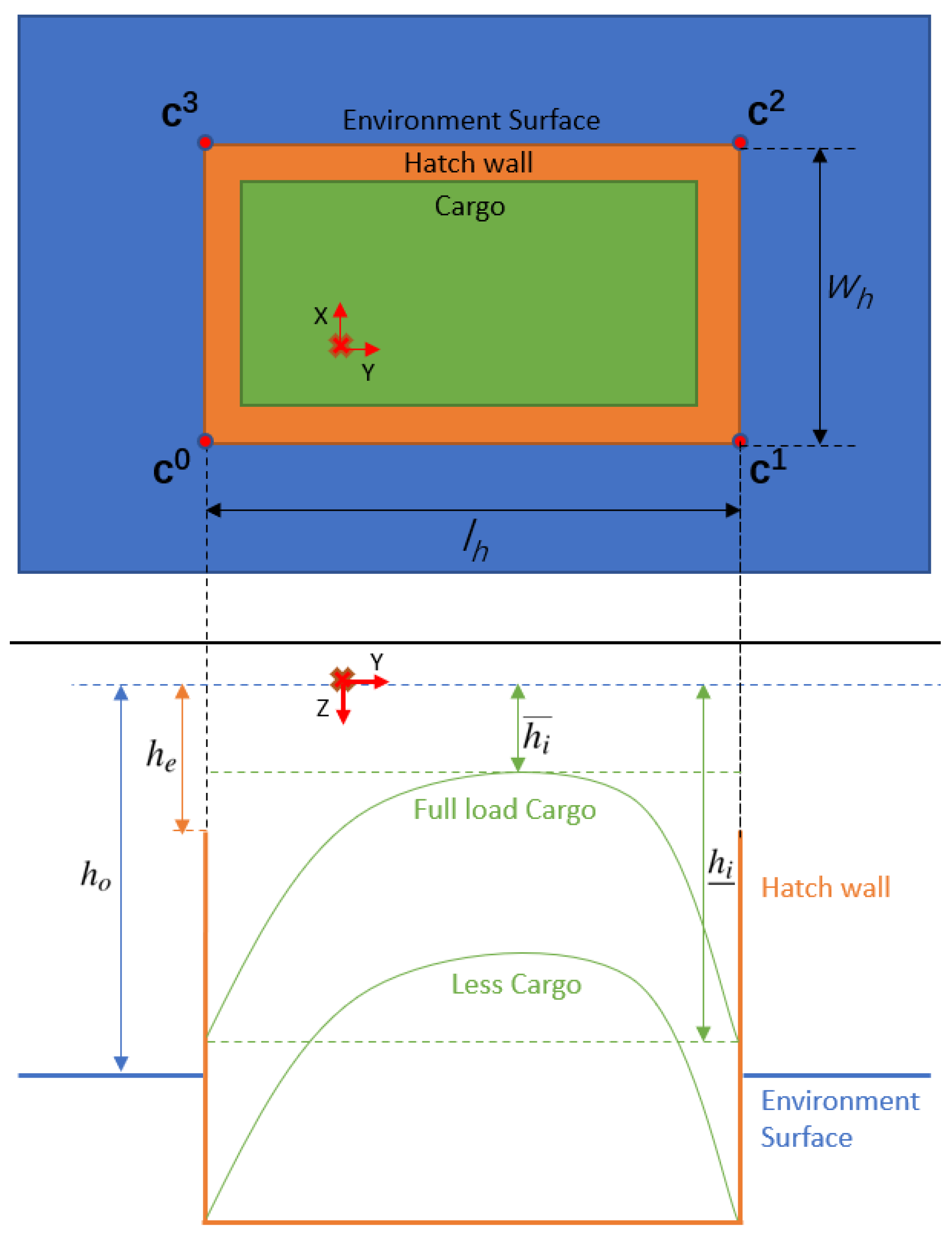
4.1. Objective and Notation

The objective of this paper is to extract the P-frame hatch edges from ${}^P\mathbf{S}$ during each cycle. The cycle has period T (see Figure 2), within which the portion $T_2$ that is devoted exclusively to processing (not scanning) should be small, so that for fixed T and $T_3$, the scan time $T_1$ can be as large as possible to provide a sufficiently dense point cloud.

Figure 4 illustrates the process of scanning the hatch and extracting the hatch edges from the scanned points during each cycle. In the following discussion, the geofenced point cloud ${}^P\mathbf{S}$ will be described as the input to the process; however, each point ${}^P{\mathbf{p}}_i\in {}^P\mathbf{S}$ is processed incrementally, at the time it is acquired, as illustrated in the flowchart.

Figure 5 depicts the structure of the P-frame point cloud ${}^P\mathbf{S}$ for one cycle. The portions of ${}^P\mathbf{S}$ corresponding to cargo in the hatch are indicated in green. The portions of ${}^P\mathbf{S}$ corresponding to hatch walls are indicated in orange. The portions of ${}^P\mathbf{S}$ corresponding to the environment surface surrounding the hatch are indicated in blue. The origin and axes of P-frame (i.e., the location of the PT and LiDAR) are shown in red.

The z-coordinate difference between the scanning system P-frame and nearest hatch edge (extracted from the point cloud) is denoted as $h_e$. The z-coordinate difference between the scanning system P-frame and the environment surrounding the hatch is denoted as $h_o$. The z-coordinate difference between the scanning system P-frame and the inner cargo highest point is denoted as $\overline{h_i}$. The z-coordinate difference between the scanning system P-frame and the inner cargo lowest point is denoted as $\underline{h_i}$. There are multiple possible scenarios for the hatch localization problem.

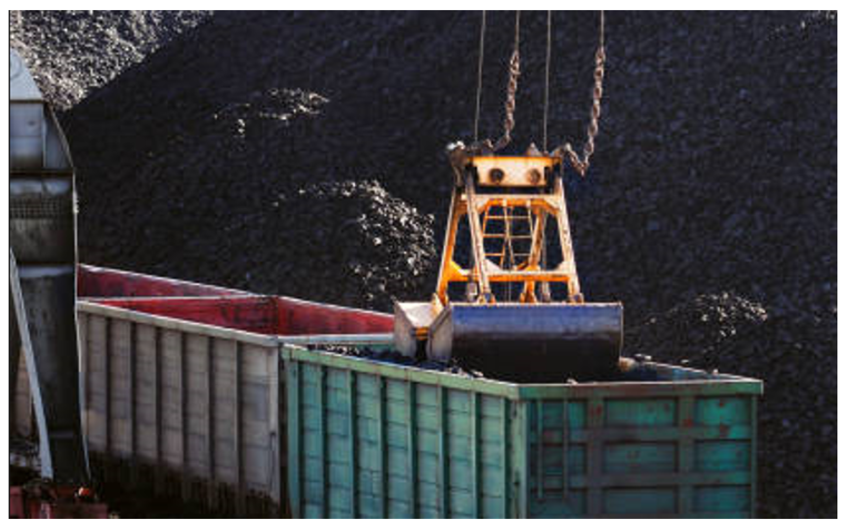
• The hatch is nearly empty, while the environment surface is low (i.e., $\overline{h_i}>h_e$ and $h_o>h_e$ ), e.g., the red train car in Figure 1.
• The hatch is nearly (or beyond) full, while the environment surface is low (i.e., $\overline{h_i}<h_e$ and $h_o>h_e$ ), e.g., the green train car in Figure 1.
• The hatch is nearly empty, while the environment surface is high (i.e., $\overline{h_i}>h_e$ and $h_o<h_e$ ), e.g., an empty ship hatch, as has been addressed in [6,7].
• The hatch is nearly (or overly) full, while the environment surface is high (i.e., $\overline{h_i}<h_e$ and $h_o<h_e$ ).

The algorithm is designed to work in all listed scenarios. Due to data availability, the experimental results in Section 6 will only consider scenarios 3 and 4.

In loading and unloading applications, the machinery enters or exits the hatch approximately along the P-frame z-axis. Therefore, determining the hatch edge lines in the x-y plane is sufficient to avoid collisions between the machinery and the hatch edges. Herein, determining the 3D hatch edge planes will be simplified to the problem of determining a 2D line in the x-y plane for each of the four edges. The corners of the hatch will be denoted by $c^j$, $j=0,1,2,3$. As shown in the top portion of Figure 5, the corner with the smallest distance to the P-frame origin is $c^0$. Starting from $c^0$, the other points are defined consecutively in counterclockwise order. The edge line connecting $c^j$ and the next counterclockwise corner defines the line parameters $e_j=({\rho }_j,{\theta }_j)$, where the $(x,y)$ coordinates of point on each line satisfy

$${\rho }_j=xcos\left({\theta }_j\right)+ysin\left({\theta }_j\right).$$

(2)

Once the hatch edges are computed, the parameters $h_e$, $h_o$, and the cargo points within the hatch can be extracted, which is useful for control and planning in cargo management. These extraction processes for these items are not described herein, as they are enabled by, but not directly related to, the process of hatch corner estimation.

The paper will use the following mathematical notation. The symbol $\lceil \mathbf{X}\rceil$ is used as the ceiling function of a vector X, which outputs a vector with the same dimension. Each element of the output vector is the smallest integer larger than or equal to the corresponding element in X. The symbol $\lfloor \mathbf{X}\rfloor$ is used as the floor function of a vector X, which outputs a vector with the same dimension. Each element of the output vector is the largest integer smaller than or equal to the corresponding element in X. The symbol $\mathbb{B}$ is used to represent a set of binary numbers.

4.2. Assumptions

The assumptions for the method described herein are as follows.

• The P-frame x–y plane is approximately parallel with the plane containing the top of the hatch. This is equivalent to stating that the P-frame z-axis points approximately perpendicular to the plane containing the top of the hatch (e.g., into the hatch).
• The P-frame origin, which is defined by the scanning system location, is within the x–y edges of the hatch so that it can scan all four hatch edge planes.
• Each hatch edge is a segment of a plane. Each plane defining an x-edge (y-edge) has a normal pointing approximately parallel to the P-frame y-axis (x-axis). This implies that the edges of the hatch rectangle are approximately aligned to the P-frame x and y axes. Therefore, the outline of the hatch in the P-frame x–y view is rectangular.
• The z-extent of the hatch edge plane is deep enough that the scanning system generates enough reflecting points on the hatch edge planes.
• Upper bounds $\overline{\ell }$ and $\overline{w}$ are known for the hatch length and width, respectively.

The hatch shape assumption limits the application to rectangular hatches. The assumption of the relative orientation of the hatch to the P-frame is satisfied by properly installing the scanning system.

4.3. Subproblems

The problem of localizing the hatch edges is divided into the following subproblems.

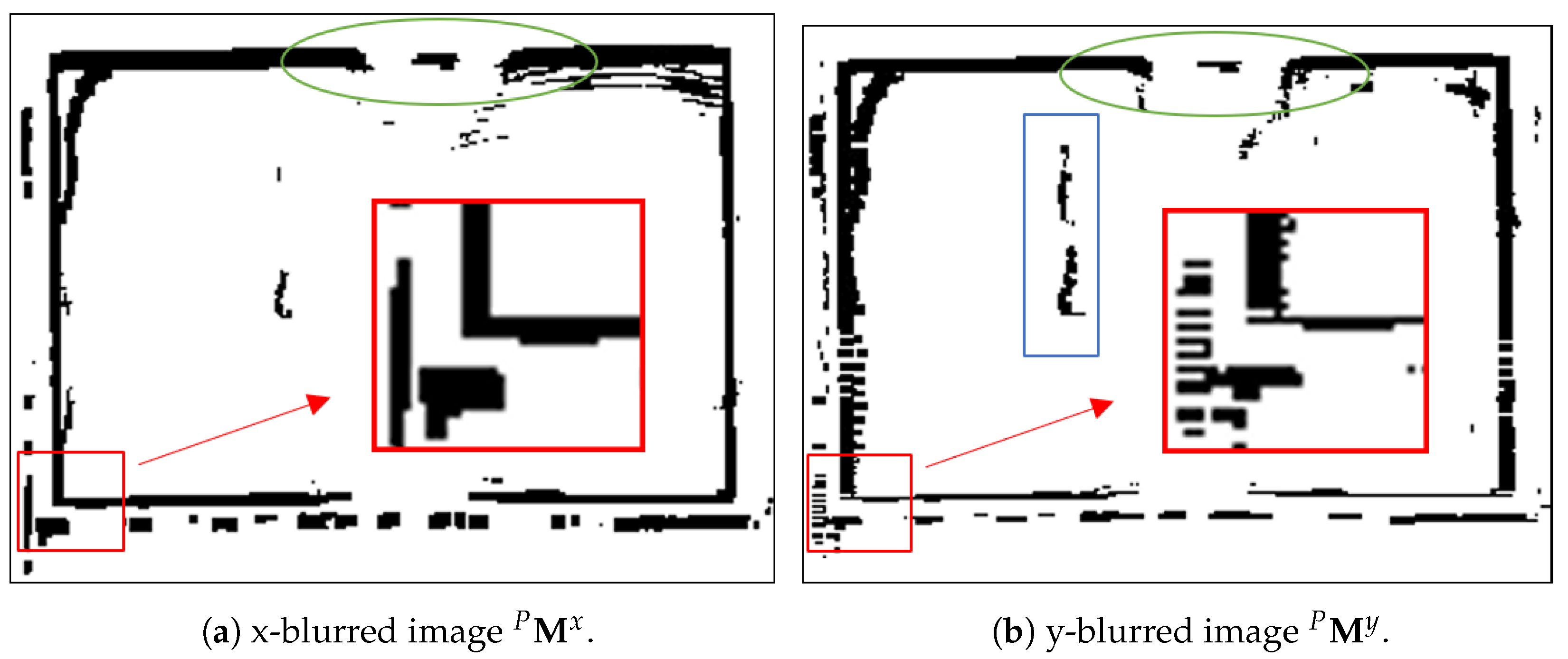
• Voxelization: Organize ${}^P\mathbf{S}$ into occupancy matrices ${}^P\mathbf{G}$, ${}^P{\mathbf{B}}^x$, and ${}^P{\mathbf{B}}^y\in {\mathbb{B}}^{N_x\times N_y\times N_z}$. Each is defined as a 3D binary matrix with $N_x$ rows, $N_y$ columns, and $N_z$ layers. The physical extent of the three voxel structures can be determined by either the extent of ${}^P\mathbf{S}$ or by a smaller geofence. Each entry ${}^P{\mathbf{G}}_{m,n,q}$ of ${}^P\mathbf{G}$ indicates whether (${}^P{\mathbf{G}}_{m,n,q}=1$) or not (${}^P{\mathbf{G}}_{m,n,q}=0$) any point of ${}^P\mathbf{S}$ is located in the volume determined by the corresponding voxel. Herein, ${}^P\mathbf{G}$, ${}^P{\mathbf{B}}^x$ and ${}^P{\mathbf{B}}^y$ will be referred to as the occupancy matrix, and the x-blurred and y-blurred occupancy matrices. The blurred occupancy matrices have utility for improving performance in image-based edge detection [36,37]. Point cloud voxelization is discussed further in Section 5.1.
• Rasterization: Convert ${}^P{\mathbf{B}}^x$ and ${}^P{\mathbf{B}}^y$ from 3D occupancy matrices to 2D occupancy matrices (i.e., images) ${}^P{\mathbf{M}}^x$, and ${}^P{\mathbf{M}}^y\in {\mathbb{B}}^{N_x\times N_y}$, such that the x and y coordinates of the hatch edges can be found by processing ${}^P{\mathbf{M}}^x$ and ${}^P{\mathbf{M}}^y$. Rasterization is discussed further in Section 5.2.
• Hatch Edge extraction: Process ${}^P{\mathbf{M}}^x$ and ${}^P{\mathbf{M}}^y$ to extract lines approximately parallel to the P-frame x-axis and y-axis, and then calculate the edge position and the hatch size from the extracted lines. Hatch edge extraction is discussed further in Section 5.3.

Voxelization is straightforward and widely used in the literature [38,39]. The focus of this paper is rasterization and hatch edge extraction.

5. Methodology

This section discusses the approaches for solving the three subproblems in Section 4.3. Section 6.2 shows images from experimental results for each step of the methodology. Note that ${}^P{\mathbf{B}}^x$, ${}^P{\mathbf{B}}^y$ are conceptual symbols defined as two collections of point pillars for theoretical discussion in this section. In the implementation, as shown in Figure 4, each point in ${}^P\mathbf{S}$ is processed to determine its voxel indices by using Equation (4) so that the layer index $q_i$ can be inserted into point pillar ${\mathbf{V}}_{m,n}$; then, if appropriate, pixel (m,n) is updated in each ${}^P{\mathbf{M}}^x$ and ${}^P{\mathbf{M}}^y$. Therefore, ${}^P\mathbf{S}$, ${\mathbf{B}}^x$, and ${}^P{\mathbf{B}}^y$ are unnecessary during the implementation of the approach.

5.1. Voxelization

The point density of the point cloud ${}^P\mathbf{S}$ is uneven, decreasing as the distance from the LiDAR increases. To achieve a desirable density near the edges of the processing region, the density may be too high in areas close to the scanning system. The process of voxelization [39] both organizes the point cloud and reduces the density where appropriate [9], without losing density in other areas. Furthermore, the occupancy matrix ${}^P\mathbf{G}$ provides an effective approach to retrieve points (i.e., voxels) within a small distance from a given voxel, or to extract all z-voxels with the same row and column indices, as will be necessary for rasterization to be discussed in Section 5.2.

The voxelization process is based on the geofence defined in Equation (1). The minimum corner of ${}^P\mathbf{G}$ is ${\underline{\mathbf{L}}}_S={[{\underline{x}}_S,{\underline{y}}_S,{\underline{h}}_e]}^{\top }$, which has the smallest value for each coordinate in the geofenced point cloud. The maximum corner of ${}^P\mathbf{G}$ is ${\overline{\mathbf{L}}}_S={[{\overline{x}}_S,{\overline{y}}_S,{\overline{h}}_e]}^{\top }$, which has the largest value for each coordinate in the geofenced point cloud. The number of voxels ${\mathbf{N}}_G={[N_x,N_y,N_z]}^{\top }$ in each dimension of ${}^P\mathbf{G}$ is calculated as

$${\mathbf{N}}_G=⌈\frac{{\overline{\mathbf{L}}}_S-{\underline{\mathbf{L}}}_S}{\mathit{c}}⌉,$$

(3)

where $\mathit{c}$ is the user-defined voxel cell size. The value of each cell ${}^P{\mathbf{G}}_{m,n,q}$ is initialized as 0.

Each point ${}^P{\mathbf{p}}_i\in {}^P\mathbf{S}$ is located within exactly one corresponding cell in ${}^P\mathbf{G}$. The row, column, and layer indices of the cell corresponding to ${}^P{\mathbf{p}}_i$ are calculated as

$${[m_i,n_i,q_i]}^{\top }=⌊\frac{{}^P{\mathbf{p}}_i-{\underline{\mathbf{L}}}_S}{c}⌋.$$

(4)

When ${}^P{\mathbf{p}}_i\in {}^P\mathbf{S}$ arrives (during $T_1$), the value of ${}^P{\mathbf{G}}_{m_i,n_i,q_i}$ is changed from 0 (unoccupied) to 1 (occupied) because this cell is occupied by point ${}^P{\mathbf{p}}_i$. The occupancy matrix only tracks if a cell is occupied without saving the coordinates of the point(s) that occupies that cell. Multiple points located in the same cell leave the value of the voxel set to 1. Because the points in LiDAR scans are discretely spaced samples along reflective surfaces, some voxels in ${}^P\mathbf{G}$ can be non-occupied even when there are (undetected) objects in the region of those voxels. However, any occupied voxel means there was an object reflecting at least one point in its region.

When coordinates are required to correspond to any voxel, a point cloud can be generated from the 3D occupancy matrix ${}^P\mathbf{G}$. Any cell ${}^P{\mathbf{G}}_{m_k,n_k,q_k}$ that has value 1 (occupied) can be converted into a 3D point by

$${}^P{\mathbf{p}}_k={\underline{\mathbf{L}}}_S+{\left[m_k+\frac{1}{2},n_k+\frac{1}{2},q_k+\frac{1}{2}\right]}^{\top }\mathit{c},$$

(5)

where ${}^P{\mathbf{p}}_k$ is the point located at the center of cell ${}^P{\mathbf{G}}_{m_k,n_k,q_k}$. The point cloud corresponding to ${}^P\mathbf{G}$ is the output of a voxel filter, which is small enough to be maintained on an industrial PC and is sufficiently dense to be used for point cloud visualization during each cycle.

The matrices ${}^P{\mathbf{B}}^x$ and ${}^P{\mathbf{B}}^y$ are introduced to improve the performance of edge detection by using image-processing methods [36,37]. The blurred occupancy matrices ${}^P{\mathbf{B}}^x$ and ${}^P{\mathbf{B}}^y$ are defined with the same dimensions and region of coverage as ${}^P\mathbf{G}$. Each matrix is initialized at the beginning of each cycle to be filled with zeroes. In addition to logging a point ${}^P{\mathbf{p}}_i$ in ${}^P{\mathbf{G}}_{m_i,n_i,q_i}$ using the indices from Equation (4), the values of entries in ${\left\{{}^P{\mathbf{B}}_{m_i+j,n_i,q_i}^x\right\}}_{j=-b_b}^{b_b}$ and ${\left\{{}^P{\mathbf{B}}_{m_i,n_i+j,q_i}^y\right\}}_{j=-b_b}^{b_b}$ are also changed to 1, where $b_b$ is a user-defined positive integer. If $b_b=0$, the three matrices ${}^P\mathbf{G}$, ${}^P{\mathbf{B}}^x$ and ${}^P{\mathbf{B}}^y$ are identical.

5.2. Rasterization

At different stages of the loading/unloading processes, the relative location will change between the cargo surface and the planes that define the hatch edges. In some point clouds, there may be no separation. Example surfaces corresponding to the full and empty hatch scenarios are depicted in Figure 6. In each subfigure, the red cross indicates the LiDAR position, and the solid green, orange, and blue curves represent LiDAR points reflected from the cargo, hatch edge plane, and surrounding environment, respectively. The gray dashed lines indicate various LiDAR ray-tracings. The black dashed lines indicate surfaces that are unscanned due to occlusion. The red dashed lines are separators between different types of pillar regions for rasterization. Those pillar regions are defined and discussed next.

All entries ${}^P{\mathbf{B}}_{m,n,q}^x$ of ${}^P{\mathbf{B}}^x$ that have the same m and n are considered as one occupancy vector ${}^P{\mathbf{V}}_{m,n}^x=\{{}^P{\mathbf{B}}_{m,n,1}^x,...,{}^P{\mathbf{B}}_{m,n,N_z}^x\}\in {\mathbb{B}}^{N_z}$. For each index pair (m, n), where $m=1,...N_x$, $n=1,...N_y$, the occupancy vector ${}^P{\mathbf{V}}_{m,n}^x$ physically represents the occupancy status of a pillar region in ${}^P{\mathbf{B}}^x$. There are five types of pillar regions, with examples shown in Figure 6. Type A includes only one cluster of points from the environment. Type B is an empty region, due to occlusion. Type C only includes one cluster of points from the cargo. Type D includes two clusters of points from both the environment and the cargo. Type E includes points from the hatch edge plane segment and cargo surface.

This section presents an approach to define the boolean value of each image pixel ${}^P{\mathbf{M}}_{m,n}^x$ by processing the occupancy vector ${}^P{\mathbf{V}}_{m,n}^x$. The goal is to set ${}^P{\mathbf{M}}_{m,n}^x$ to 1 for type E and 0 for types A–D. For the rest of this section, the subscripts m and n, and the superscripts P and x of ${}^P{\mathbf{V}}_{m,n}^x$ are dropped to simplify the notation. Therefore, the representation of the occupancy vector ${}^P{\mathbf{V}}_{m,n}^x$ is simplified in this section as $\mathbf{V}=\{v_1,...,v_{N_z}\}$.

The occupancy status in V is naturally ordered from the smallest to the largest z. The value of each element in V indicates if any surface was scanned in the voxel corresponding to that z-value in the pillar. The property that LiDAR points are discretely spaced in ${}^P\mathbf{S}$ also applies to V. Let $l_{m,n}^V$ be the length of the longest block of consecutively filled cells in ${\mathbf{V}}_{m,n}$, allowing for gaps with tolerance of $b_v$ pixels, where $b_v$ is a user-defined non-negative integer. For example, given a vector $\mathbf{V}={[0,1,1,0,1,0,0,1]}^{\top }$ and a tolerance on one ‘0’ for a gap, there are two blocks in the vector, i.e., the second to the fifth terms and the eighth term. Therefore, the length of the longest block $l_{m,n}^V$ equals the length of the first block: $l_{m,n}^{\mathbf{V}}=4$. Given Assumption 3, an occupancy vector V of the pillar region of Type E is expected to have a higher $l_{m,n}^V$ than a pillar in regions of types A–D. With a lower bound $b_e$ on the z-direction extent of the hatch edge, the value of $l_{m,n}^V$ is expected to have a value of at least $\frac{b_e}{c}$ for a pillar in a Type-E region. Therefore, the value of each ${}^P{\mathbf{M}}_{m,n}^x$ in ${}^P{\mathbf{M}}^x$ is

$${}^P{\mathbf{M}}_{m,n}^x=\left\{\begin{array}{cc}1,\hfill & \mathrm{if}{l}_{m,n}^V\ge \frac{b_e}{c}\hfill \\ 0,\hfill & \mathrm{otherwise}.\hfill \end{array}\right.$$

(6)

An identical process is applied to convert ${}^P{\mathbf{B}}^y$ to ${}^P{\mathbf{M}}^y$. The ‘1’s in ${}^P{\mathbf{M}}^x$ and ${}^P{\mathbf{M}}^y$ indicate those entries detected as candidate points for the hatch edge. Those candidate points will be used to determine the hatch edge position in Section 5.3.

5.3. Hatch Edge Extraction

Assumption 3 implies that the hatch x-edges will be represented in ${}^P{\mathbf{M}}^x$ as vertical lines and y-edges in ${}^P{\mathbf{M}}^y$ as horizontal lines. This section discusses extracting lines corresponding to the hatch edges from ${}^P{\mathbf{M}}^x$ and ${}^P{\mathbf{M}}^y$. The method is presented only for ${}^P{\mathbf{M}}^x$. The approach applies to ${}^P{\mathbf{M}}^y$ by analogy.

The HT is applied to ${}^P{\mathbf{M}}^x$ with two parameters: $\rho$ and $\theta$ [28]. The hatch edge lines are represented by Equation (2). All ${}^P{\mathbf{M}}^x$ image pixels with value 1 participate in HT voting for candidate lines. Voting occurs during $T_1$, at the time that the pixel is set to 1. The distance range and angular range of the HT are $\rho \in ({\underline{y}}_S,{\overline{y}}_S)$, and $\theta \in (\frac{\pi }{2}-{\delta }_x,\frac{\pi }{2}+{\delta }_x)$. The resolution of $\rho$ for vote accumulation is the cell size c. Given Assumption 3, the magnitude of the misalignment between the hatch edge lines and P-frame axes is small, so that ${\delta }_x$ is a small angle with limits determined by the application conditions. The resolution of $\theta$ was selected as $0.002$ rad.

The parameters of the extracted candidate lines with sufficient votes are denoted as $({\rho }_i^x,{\theta }_i^x)$ for $i=1,\dots ,N_E^x,$ where $N_E^x$ is the number of extracted lines from ${}^P{\mathbf{M}}^x$ and the lines are sorted in ascending order based on the value of line parameters ${\rho }_i^x$: ${\rho }_1^x\le \dots \le {\rho }_{N_E^x}^x$. Based on Assumption 2, the two lines nearest to and on opposite sides of the origin should correspond to the hatch edges $e_1$ and $e_3$. Define

$$i_1=arg\underset{{\rho }_i<0}{max}\left({\rho }_i\right)\mathrm{and}{i}_3=arg\underset{{\rho }_i>0}{min}\left({\rho }_i\right).$$

The line defining $e_1$ is parameterized as $({\rho }_{i_1},{\theta }_{i_1})$. The line defining $e_3$ is parameterized as $({\rho }_{i_3},{\theta }_{i_3})$.

The edges parallel to the P-frame y-axis are similarly extracted to define $e_0$ and $e_2$ by processing ${}^P{\mathbf{M}}^y$ in a manner analogous to that described above.

5.4. Summary of Constant Parameters

This section discusses the various constants involved in the method and provides advice about selecting their values.

• Geofence parameters${\underline{x}}_S$, ${\overline{x}}_S$, ${\underline{y}}_S$, ${\overline{y}}_S$, ${\underline{h}}_e$, ${\overline{h}}_e$ $\left(meters\right)$: These constants are used in Equation (1) to define the geofence. The purpose is to remove points that are not relevant while retaining all hatch edge points even as the hatch moves between cycles. The values are user-defined based on local knowledge of hatch motion.
• Cell size$c\left(meters\right)$: The cell size is used in the definition of the three occupancy matrices ${}^P\mathbf{G}$, ${}^P{\mathbf{B}}^x$, and ${}^P{\mathbf{B}}^y$. It determines the resolution of these voxelized point clouds. For a given point cloud region, the memory requirements of each occupancy matrix scales cubically with $\frac{1}{c}$. Larger structures also require longer processing time. The cell size needs to be small enough to meet the localization accuracy requirement and large enough to be comparable with the accuracy of the raw data. Herein, the cell size is 5 cm through all experiments, which is comparable with the accuracy of the raw LiDAR range data.
• Parameters for gaps:$b_b,b_v$ $\left(pixels\right)$: The purpose of these parameters is to improve edge extraction performance [36,37]. These constants are used in Section 5.1 and Section 5.2.
• Hatch edge plane depth lower bound$b_e$ $\left(meters\right)$: This constant is used in Equation (6) to check whether each occupancy vector (i.e., pillar) is deep enough in the z-direction to be regarded as a piece of a hatch edge plane. It needs to be large enough to reject small plane segments and small enough that hatch edge points are recognized.
• Hough transform angular search range${\delta }_x$ $\left(radians\right)$: This constant is used in Section 5.3 to limit the HT angular search to the small range required due to Assumption 3. This constant must be large enough to account for misalignment of the hatch edges with the P-frame x and y axes. If it is too small, hatch edges could be missed. As it is increased, the HT computation time will increase.

6. Experimental Results

This section discusses the experimental setup and results. The LiDAR used to perform the experiments is a Quanergy M8. The PT rotation pattern designed for the M8 is discussed in Section 6.1. With this setup, the detailed results from each step of the approach are shown in Section 6.2. Section 6.3 introduces the metrics for evaluating sequential results of one dataset in Section 6.4 and multiple datasets in Section 6.5.

6.1. Scanning Patterns

A LiDAR mounted on a PT allows two independent basic scanning patterns: panning and tilting. The following subsections discuss the positive and negative aspects of each for generating the unorganized point cloud ${}^P\mathbf{S}$ within the context of the time constraint imposed by the cyclic operation. For the cyclic scanning discussed relative to Figure 2, the time budget for $T_1+T_2$ is 15 s. In this section, for the purpose of calculating point cloud resolution, we assume $T_1=12$ s. This is the typical time required for the crane to dump the cargo it extracted during the previous cycle, which is the time available to accumulate a point cloud.

6.1.1. Circular Scanning: Pan Rotation

When the PT body pans around the P-frame z-axis while the tilt angle is zero, it results in a circular scanning pattern, as shown in Figure 7. The point cloud ${}^P\mathbf{S}$ will have a center point below the scanning system. The density of points is highest near the center point and decreases as the distance to the center point increases. The PT must rotate by at least 180 degrees to scan the entire hatch once. Therefore, a pan rotation rate of ${\omega }_p={\displaystyle \frac{180}{T_1}}=15$ deg/s is required. The LiDAR is configured with a frame rate $f=20$ Hz such that the pan angle difference between two sequential scanlines is ${\gamma }_p={\displaystyle \frac{{\omega }_p}{f}}=0.75$ degrees. The angular resolution of points within each scanline is approximately ${\gamma }_s=0.14$ degrees.

6.1.2. Swipe Scanning: Tilt Rotation

When the pan angle is constant and the tilt angle changes from a maximum to a minimum value, a swipe pattern results. If the LiDAR scanline is approximately aligned with a hatch edge (e.g., 0, or 180 degrees) the tilt angle change causes the laser scanline to traverse along the perpendicular hatch edge from one extreme to the other. Therefore, the accumulated point cloud ${}^P\mathbf{S}$ will consist of scanlines approximately parallel in a bird-eye’s view. For example, in Figure 8, the scanning system swipes from the first scanline to the last scanline. Therefore, with the same time budget $T_1$ and a maximum initial tilt range of 90 degrees, the tilt rotation speed is at least ${\omega }_t=\frac{90}{T_1}=7.5$ deg/s. For the experiments that follow, the PT tilts at its speed of 8 deg/s. The LiDAR frame rate $f=20$ Hz; therefore, the tilt angle change between two scanlines is ${\gamma }_t=\frac{8}{f}\approx 0.4$ degrees.

6.1.3. Scanning Pattern Comparison

The gaps in ${}^P\mathbf{S}$ are numerically analyzed in this section. To consider the worst case, the calculation is based on one rotating laser. The gaps between consecutive points in one scanline ($d_r$) and the gaps between scanlines ($d_{p1}$) are considered. The value of $d_r$ is the same in both cases. For a hatch that is approximately 30 m from the scanning system, $d_r=30{\gamma }_s=0.07$ m.

For a pan rotation, as in Figure 7, the distance between hatch edge points is calculated as $d_{p1}=R_p{\gamma }_p$, where $R_p$ is the projection of R onto the x-y plane. For the area of the A-side plane closest to the origin, the distance is $d_{p1}=12{\gamma }_p=0.05$ m. For the pan rotation, the two types of gaps are both small and have similar magnitudes.

For tilt rotation (i.e., Figure 8), the gap between two adjacent scanlines depends on the angle of incidence of the laser with the hatch side-edge wall (i.e., either side A or C in Figure 8),

$$d_{p2}=\frac{sin\left({\gamma }_t\right)}{sin(\frac{\pi }{2}-\psi -{\gamma }_t)}R,$$

(7)

where R is the range of the higher scanline, $\psi$ is the angle of incidence between the laser and the vertical wall for the higher scanline, and ${\gamma }_t$ is the tilt-angle difference (i.e., the angle between the two laser scanlines). This equation is derived by using the law of sines. Typically, $\psi \approx 80$ degrees for hatch edge planes, yielding $d_{p2}=1.69$ m. When the laser is on a surface with a negligible angle of incidence (e.g., cargo or hatch surround), the between-scanline gap is approximately $d_{p3}=R{\gamma }_t=0.21$ m.

6.2. Processing of One Scan

This section discusses the intermediate results during one cycle of point cloud processing, using a dataset for a full hatch. The voxelized point cloud ${}^P\mathbf{G}$ is shown in Figure 8. Note that the number of hatch edge points is a small percentage of the overall point cloud ${}^P\mathbf{G}$, especially for sides A and C. Therefore, methods such as RANSAC are unlikely to succeed.

The rasterization results ${}^P{\mathbf{M}}^x$ and ${}^P{\mathbf{M}}^y$ are shown in Figure 9. Each pixel represents a 5 × 5 cm${}^2$ area. The black pixels in ${}^P{\mathbf{M}}^x$ and ${}^P{\mathbf{M}}^y$ define the candidate y and x hatch edge points. The image in Figure 9a was blurred in the vertical direction, and the image in Figure 9b was blurred in the horizontal direction.

Because the hatch length is known to exceed 10 m, successful HT edge line segment candidates that are shorter than 5 m are discarded. Corresponding to Figure 9a, the successful HT near vertical lines candidates are shown as yellow lines in Figure 10. Similarly, the near horizontal line candidates extracted from ${}^P{\mathbf{M}}^y$ of Figure 9b are shown in Figure 10 as cyan lines. The 5-m length requirement eliminates false-positive line results. For example, the cargo area indicated by the blue rectangle is steep enough that some pixels in the area are recognized as hatch edge candidates in ${}^P\mathbf{M}$, but removed by the line length threshold.

Figure 10 depicts several overlapping line edge candidates, each drawn with a line width corresponding to the cell size. Figure 11a,b show the x and y placement of the overlapping lines. Because a main goal of hatch localization herein is avoiding collisions between the crane and the hatch edge, the two vertical lines nearest to and on opposite sides of the origin are selected. For Figure 10, the distances from the selected vertical lines to the origin (i.e., LiDAR location) are −7.65 m (side B) and 15.90 m (side D). Similarly, the distances from the LiDAR to the hatch edges on sides A and C are −5.45 m and 9.90 m for Figure 10b.

6.3. Assessment Metrics

The ground-truth hatch edge locations are unknown and time-varying; therefore, they cannot be used for accuracy assessment. Instead, when it is available, the constant hatch length and width will be used to assess accuracy. These are easily computed by differencing the hatch edge positions.

For the example in Section 6.2, the reference hatch size in this case is known to be 23.75 × 15.3 m. The experiment measurements are 23.55 × 15.35 m. Therefore, the size error is 0.2 m in the x-direction and 0.05 meters in the y-direction, which surpasses the accuracy requirement of errors less than 0.5 m for anti-collision purposes.

When a hatch edge is stationary, performance can also be assessed by considering the hatch edge position standard deviation (PSTD) between different cycles processed independently. When a hatch edge is moving, performance can be assessed by considering the average hatch size error (ASH), the maximum hatch size error (MSH), and the hatch size standard deviation (HSTD).

6.4. Tracking Motion over Sequential Scans

This section demonstrates the ability to track hatch motion by showing the hatch localization results of sequential scans of the same dataset used in Section 6.2. The point clouds accumulated in sequential cycles are processed independently to extract the hatch edge locations as shown in Figure 12a–d. During the period of this dataset, after the tenth cycle, the hatch moved in the x-direction relative to the P-frame. The resolution of the hatch edge position results is determined by the cell size c; therefore, the minimum separation between results in Figure 12 is 5 cm.

Figure 12a,b show the hatch x-edge positions measured per cycle. Figure 12c,d show the hatch y-edge positions measured per cycle. Figure 12e,f display the reference (red line) and per cycle computed hatch length (blue markers) in the x and y directions, respectively.

Because the hatch did move in the x-direction, only the x-length consistency can be assessed. The x-length estimation performance metrics are ASH is −0.05 m, MSH is −0.2 m, and HSTD is 0.06 m because the hatch did not move in y-direction. The estimated y-edge locations are essentially constant with position standard deviation (PSTD) of 0.04 m (0.03 m) for the y-negative (y-positive) edge. Concerning the y-length: ASH is −0.18 m, MSH is −0.25 m, and HSTD is 0.05 m.

6.5. Statistical Results over Multiple Datasets

This section presents and discusses the statistical hatch localization results in

Table 1. Hatch extraction statistical results over 608 cycles from 24 datasets.

Dataset	# Cycle	Hatch- Cargo Gap (m)	Hatch Size (m)						Hatch Edge Position (m)
			X			Y
			ASH	MSH	HSTD	ASH	MSH	HSTD	X- PSTD	X+ PSTD	Y- PSTD	Y+ PSTD
1	6	7.15	0.03	0.05	0.03	−0.01	−0.05	0.02	0.03	0.00	0.03	0.03
2	7	7.15	−0.22	−0.30	0.06	−0.21	−0.25	0.05	0.03	0.05	0.02	0.04
3	10	8.35	0.03	0.08	0.03	0.07	0.10	0.03	0.03	0.02	0.03	0.00
4	12	5.45	0.03	0.10	0.03	−0.05	−0.10	0.03	0.03	0.01	0.02	0.03
5	13	OL	−0.03	−0.20	0.12	−0.17	−0.25	0.06	0.08	0.07	0.04	0.03
6	14	4.15	−0.21	−0.32	0.07	−0.14	−0.16	0.03	0.05	0.03	0.02	0.02
7	27	6.20	−0.27	−0.34	0.05	−0.17	−0.25	0.06	0.07	0.05	0.06	0.05
8	29	12.05	−0.09	−0.14	0.06	0.06	0.10	0.03	0.04	0.03	0.03	0.02
9	34	9.40	−0.01	−0.15	0.05	0.03	0.10	0.03	0.05	0.02	0.03	0.03
10	37	5.25	0.03	0.09	0.04	0.10	0.14	0.02	0.03	0.03	0.02	0.01
11	39	6.35	−0.22	−0.27	0.03	0.18	0.25	0.04	0.03	0.03	0.03	0.03
12	48	10.15	0.00	0.03	0.03	0.14	0.25	0.04	0.03	0.04	0.03	0.03
13	51	6.55	−0.06	−0.17	0.05	−0.03	−0.10	0.03	0.03	0.04	0.04	0.03
14	53	6.05	−0.15	−0.27	0.07	−0.18	−0.24	0.04	0.09	0.06	0.02	0.04
15	13	4.35	0.08	0.05	0.03	−0.01	−0.05	0.03	0.02	0.02	0.03	0.02
16	16	10.85	0.06	0.20	0.09	0.06	0.10	0.06	0.03	0.09	0.04	0.08
17	16	7.10	−0.04	−0.07	0.03	0.02	0.10	0.04	0.03	0.02	0.05	0.02
18	17	11.95	0.05	0.10	0.03	0.05	0.10	0.04	0.03	0.03	0.03	0.02
19	20	OL	−0.07	−0.25	0.11	−0.15	−0.25	0.05	0.09	0.05	0.03	0.03
20	23	7.00	−0.21	−0.27	0.03	−0.14	−0.20	0.05	0.03	0.03	0.04	0.04
21	29	6.10	−0.09	−0.16	0.04	−0.02	−0.06	0.03	0.04	0.03	0.02	0.02
22	29	8.45	−0.01	−0.05	0.03	−0.06	−0.10	0.04	0.06	0.06	0.06	0.04
23	32	6.30	0.04	0.10	0.05	−0.01	0.10	0.04	0.03	0.03	0.03	0.03
24	33	8.30	−0.05	−0.12	0.04	0.04	0.11	0.03	0.04	0.03	0.02	0.02

for 608 cycles total from 24 datasets (i.e., hatches). The datasets are categorized into two groups as indicated by the horizontal dashed line. Datasets 1-14 are collected when the hatch and scanning system are both stationary. Datasets 15-24 each include cycles before and after relative movement between the hatch and scanning system. Each row represents the statistical results of one dataset by using the metrics defined in Section 6.3. The first two columns define the name of and number of cycles in the dataset. Column 3 presents the approximate smallest z difference between hatch points and cargo points. Datasets 5 and 19 are full-hatch datasets, for which the hatch and cargo overlap in some regions. In these instances, the hatch-cargo gap is recorded as ‘OL’ for overlapping. Columns 4 through 9 contain the hatch size statistics (i.e., ASH, MSH and HSTD). The last four columns show the PSTD for each hatch edge position estimate.

Note that there are instances where standard deviations are zero (e.g., Dataset 1 $x+$ PSTD). This is due to voxelization and the hatch edge position resolution of 5 cm.

The hatch edge extraction accuracy is consistent, with a maximum PSTD of 0.09 m. Possible causes of the position variance include the accuracy of the raw LiDAR measurement being 5 cm and the voxelization resolution being 5 cm.

The maximum MSH among all cycles of all datasets is −0.34 m in the x-direction and −0.25 m in the y-direction. Furthermore, the ASH and HSTD are −0.27 and 0.12 m (−0.21 and 0.06 m) in the x-direction (y-direction) in the worst case. Possible causes of the size estimation error include choosing the closest lines to the P-frame origin, which prioritizes safety over accuracy, PT measurement errors and latency, and inaccurate calibration.

During the computation of the results in Table 1, the computation time $T_2$ was recorded, between the end of the point cloud accumulation during $T_1$ and the availability of the hatch localization results. The average (maximum) delay was 2.69 (4.29) ms. This delay is negligible compared with the point cloud accumulation time of $T_1\approx 12$ s and the cycle time of approximately 30 s.

7. Discussion

A few topics merit additional discussion.

7.1. PT Pattern Determination

The PT rotation pattern must be specifically designed based on the LiDAR used. The goals are to reach a large enough hatch edge point density within the time constraints of the cyclic operation to find the hatch edge accurately and reliably in all scans.

From the sole perspective of point density on the hatch edge, the pan operation is clearly superior. However, another consideration is the time to scan the hatch. A typical change in tilt to scan a hatch is about 30 degrees. For example, in Figure 8, the hatch edges are located about $x=10$, $y=-6$, and $z=30$ m from the LiDAR. Therefore, the change in tilt angle to scan the hatch is approximately $atan(10,30)-atan(-6,30)=29.7$ degrees. With an angular rate of ${\omega }_t=8$ deg/s, the time to change tilt by 30 degrees is only 3.75 s. The circular scan time cannot be reduced below 12 s, because it has to finish a 180-degree pan-rotation. In this paper, the swipe scanning is preferred for the M8 LiDAR as it allows more cycles per hour.

7.2. Cargo-Hatch Overlap

The overlap between cargo and hatch edge wall (see the area marked by the green ellipse in Figure 8) appears when the hatch is fully loaded; therefore, there is no 3D plane that can separate the hatch and cargo points. This implies the approaches of [6,7] cannot be used directly for extracting the hatch when it is full because they assume an input point cloud of the hatch without points from the cargo.

Furthermore, the vertical extent of the hatch edge plane in those areas was not completely scanned. This reduces the z-extent of the corresponding pillars, which may cause rasterization to fail to detect portions of the hatch edge in those regions (see the green ellipses in Figure 9). This emphasizes the necessity of Assumption 4 for the approach of this paper.

7.3. Hatch Size Determination Strategy

The hatch size estimates are smaller than the known reference values for most cycles in Figure 12e,f. Due to measurement noise and voxel resolution, multiple candidate lines are found as depicted in Figure 10. The design choice to select the two lines nearest to and on opposite sides of the origin, to attain a low risk of collisions, causes this underestimation of the hatch length. The underestimation is acceptable as its magnitude is less that the desired accuracy of 0.5 m.

To present the accuracy results clearly, the hatch localization results are discussed for each cycle independently. In actual applications, the results could be filtered across time (i.e., cycles) to reduce variation, estimate motion, and remove outlier measurements.

8. Conclusions

This paper considers the problem of determining the time-varying location of a cargo hatch within the time constraints applicable to cyclic transloading operations. A novel approach is presented and evaluated by using data from a LiDAR mounted on a pan-tilt scanning system. A point cloud is generated during the time period when the crane is not above the hatch due to its dumping of extracted cargo from the previous cycle. While the point cloud is being accumulated, the incoming points are voxelized, converted into point pillars that are rasterized, and Hough transform line candidate voting takes place. At the completion of the scanning process, the best hatch edge lines are extracted from the Hough transform results. This approach completes the majority of the computation while scanning takes place, so that the hatch edge location estimates for the current cycle are rapidly available after the scan completes.

The approach has been evaluated with 608 cycles from 24 different hatches by using real transloading datasets. The results show that the approach performs reliably and accurately for various hatch fullness levels (see column 3 in Table 1). Therefore, the approach can be applied from the early unloading through the late loading stages of transloading work.

The following future research topics are of interest.

• The case of an exactly full hatch is rare in transloading. When it occurs, it causes severe cargo-hatch overlap as discussed in Section 7.2. Currently, manual unloading proceeds until enough of the hatch edge is exposed. Potential ideas to solve this special case include the detection of point cloud features (e.g., surface roughness or curvature) that distinguish cargo from hatch or augmentation of an additional sensor (e.g., camera).
• The duration of a transloading task is usually long; therefore, it is interesting to develop the algorithm to filter across time as mentioned in Section 7.3.
• Both the development and the use of an active acoustic sensor able to resolve the range and angle of points along a reflecting surface relative to the sensor would be very interesting.

References

- Mi, C.; Zhang, Z.W.; Huang, Y.F.; Shen, Y. A fast automated vision system for container corner casting recognition. J. Mar. Sci. Technol. 2016, 24, 54–60. [Google Scholar] [CrossRef]
- Shen, Y.; Mi, W.; Zhang, Z. A Positioning Lockholes of Container Corner Castings Method Based on Image Recognition. Pol. Marit. Res. 2017, 24, 95–101. [Google Scholar] [CrossRef] [Green Version]
- Vaquero, V.; Repiso, E.; Sanfeliu, A. Robust and Real-Time Detection and Tracking of Moving Objects with Minimum 2D LiDAR Information to Advance Autonomous Cargo Handling in Ports. Sensors 2018, 19, 107. [Google Scholar] [CrossRef] [Green Version]
- Yoon, H.J.; Hwang, Y.C.; Cha, E.Y. Real-time container position estimation method using stereo vision for container auto-landing system. In Proceedings of the International Conference on Control, Automation and Systems, Gyeonggi-do, Korea, 27–30 October 2010; pp. 872–876. [Google Scholar] [CrossRef]
- Mi, C.; Huang, Y.; Liu, H.; Shen, Y.; Mi, W. Study on Target Detection & Recognition Using Laser 3D Vision Systems for Automatic Ship Loader. Sens. Transducers 2013, 158, 436–442. [Google Scholar]
- Mi, C.; Shen, Y.; Mi, W.; Huang, Y. Ship Identification Algorithm Based on 3D Point Cloud for Automated Ship Loaders. J. Coast. Res. 2015, 73, 28–34. [Google Scholar] [CrossRef]
- Miao, Y.; Li, C.; Li, Z.; Yang, Y.; Yu, X. A novel algorithm of ship structure modeling and target identification based on point cloud for automation in bulk cargo terminals. Meas. Control. 2021, 54, 155–163. [Google Scholar] [CrossRef]
- Lang, A.H.; Vora, S.; Caesar, H.; Zhou, L.; Yang, J.; Beijbom, O. PointPillars: Fast Encoders for Object Detection From Point Clouds. In Proceedings of the Conference on Computer Vision and Pattern Recognition, Long Beach, CA, USA, 15–20 June 2019; pp. 12689–12697. [Google Scholar] [CrossRef] [Green Version]
- Hackel, T.; Wegner, J.D.; Schindler, K. FAST SEMANTIC SEGMENTATION OF 3D POINT CLOUDS WITH STRONGLY VARYING DENSITY. ISPRS Ann. Photogramm. Remote Sens. Spat. Inf. Sci. 2016, III-3, 177–184. [Google Scholar] [CrossRef] [Green Version]
- Li, Y.; Olson, E.B. A General Purpose Feature Extractor for Light Detection and Ranging Data. Sensors 2010, 10, 10356–10375. [Google Scholar] [CrossRef] [Green Version]
- Sun, J.; Li, B.; Jiang, Y.; Wen, C.y. A Camera-Based Target Detection and Positioning UAV System for Search and Rescue (SAR) Purposes. Sensors 2016, 16, 1778. [Google Scholar] [CrossRef]
- Symington, A.; Waharte, S.; Julier, S.; Trigoni, N. Probabilistic target detection by camera-equipped UAVs. In Proceedings of the International Conference on Robotics and Automation, Anchorage, AK, USA, 3–7 May 2010; pp. 4076–4081. [Google Scholar] [CrossRef] [Green Version]
- Wang, W.; Liu, J.; Wang, C.; Luo, B.; Zhang, C. DV-LOAM: Direct Visual LiDAR Odometry and Mapping. Remote Sens. 2021, 13, 3340. [Google Scholar] [CrossRef]
- Hammer, M.; Hebel, M.; Borgmann, B.; Laurenzis, M.; Arens, M. Potential of LiDAR sensors for the detection of UAVs. In Proceedings of the Laser Radar Technology and Applitions XXIII, Orlando, FL, USA, 17–18 April 2018; p. 4. [Google Scholar] [CrossRef]
- Rachman, A.A. 3D-LIDAR Multi Object Tracking for Autonomous Driving: Multi-target Detection and Tracking under Urban Road Uncertainties. Master’s Thesis, TU Delft Mechanical, Maritime and Materials Engineering, Esbjerg, Danmark, 2017. [Google Scholar]
- Tarsha Kurdi, F.; Gharineiat, Z.; Campbell, G.; Awrangjeb, M.; Dey, E.K. Automatic Filtering of Lidar Building Point Cloud in Case of Trees Associated to Building Roof. Remote Sens. 2022, 14, 430. [Google Scholar] [CrossRef]
- Ren, Z.; Wang, L. Accurate Real-Time Localization Estimation in Underground Mine Environments Based on a Distance-Weight Map (DWM). Sensors 2022, 22, 1463. [Google Scholar] [CrossRef]
- Xue, G.; Wei, J.; Li, R.; Cheng, J. LeGO-LOAM-SC: An Improved Simultaneous Localization and Mapping Method Fusing LeGO-LOAM and Scan Context for Underground Coalmine. Sensors 2022, 22, 520. [Google Scholar] [CrossRef] [PubMed]
- Bocanegra, J.A.; Borelli, D.; Gaggero, T.; Rizzuto, E.; Schenone, C. A novel approach to port noise characterization using an acoustic camera. Sci. Total. Environ. 2022, 808, 151903. [Google Scholar] [CrossRef]
- Remmas, W.; Chemori, A.; Kruusmaa, M. Diver tracking in open waters: A low-cost approach based on visual and acoustic sensor fusion. J. Field Robot. 2021, 38, 494–508. [Google Scholar] [CrossRef]
- Svanstrom, F.; Englund, C.; Alonso-Fernandez, F. Real-Time Drone Detection and Tracking With Visible, Thermal and Acoustic Sensors. In Proceedings of the 2020 25th International Conference on Pattern Recognition (ICPR), Milan, Italy, 10–15 January 2021; pp. 7265–7272. [Google Scholar] [CrossRef]
- Gong, L.; Zhang, Y.; Li, Z.; Bao, Q. Automated road extraction from LiDAR data based on intensity and aerial photo. In Proceedings of the 3rd International Congress on Image and Signal Processing, Yantai, China, 16–18 October 2010; pp. 2130–2133. [Google Scholar] [CrossRef]
- Raj, T.; Hashim, F.H.; Huddin, A.B.; Ibrahim, M.F.; Hussain, A. A Survey on LiDAR Scanning Mechanisms. Electronics 2020, 9, 741. [Google Scholar] [CrossRef]
- Fischler, M.A.; Bolles, R.C. Random sample consensus: A paradigm for model fitting with applications to image analysis and automated cartography. Commun. ACM 1981, 24, 381–395. [Google Scholar] [CrossRef]
- Yang, L.; Li, Y.; Li, X.; Meng, Z.; Luo, H. Efficient plane extraction using normal estimation and RANSAC from 3D point cloud. Comput. Stand. Interfaces 2022, 82, 103608. [Google Scholar] [CrossRef]
- Adams, R.; Bischof, L. Seeded region growing. IEEE Trans. Pattern Anal. Mach. Intell. 1994, 16, 641–647. [Google Scholar] [CrossRef] [Green Version]
- Ballard, D.H. Generalizing the Hough transform to detect arbitrary shapes. Pattern Recognit. 1981, 13, 111–122. [Google Scholar] [CrossRef] [Green Version]
- Duda, R.O.; Hart, P.E. Use of the Hough transformation to detect lines and curves in pictures. Commun. ACM 1972, 15, 11–15. [Google Scholar] [CrossRef]
- Hulik, R.; Spanel, M.; Smrz, P.; Materna, Z. Continuous plane detection in point-cloud data based on 3D Hough Transform. J. Vis. Commun. Image Represent. 2014, 25, 86–97. [Google Scholar] [CrossRef]
- Choi, S.; Kim, T.; Yu, W. Performance Evaluation of RANSAC Family. In Proceedings of the British Machine Vision Conference, London, UK, 7–10 September 2009; pp. 81.1–81.12. [Google Scholar] [CrossRef] [Green Version]
- Vo, A.V.; Truong-Hong, L.; Laefer, D.F.; Bertolotto, M. Octree-based region growing for point cloud segmentation. ISPRS J. Photogramm. Remote Sens. 2015, 104, 88–100. [Google Scholar] [CrossRef]
- Zhan, Q.; Liang, Y.; Xiao, Y. Color-based segmentation of point clouds. Laser Scanning 2009, 38, 155–161. [Google Scholar]
- Tarsha-Kurdi, F.; Landes, T.; Grussenmeyer, P. Hough-transform and extended ransac algorithms for automatic detection of 3D building roof planes from Lidar data. In Proceedings of the ISPRS Workshop on Laser Scanning and SilviLaser, Espoo, Finland, 12–14 September 2007; Volume 36, pp. 407–412. [Google Scholar]
- Ali, W.; Liu, P.; Ying, R.; Gong, Z. A Feature Based Laser SLAM Using Rasterized Images of 3D Point Cloud. IEEE Sens. J. 2021, 21, 24422–24430. [Google Scholar] [CrossRef]
- Guiotte, F.; Pham, M.T.; Dambreville, R.; Corpetti, T.; Lefevre, S. Semantic Segmentation of LiDAR Points Clouds: Rasterization Beyond Digital Elevation Models. IEEE Geosci. Remote Sens. Lett. 2020, 17, 2016–2019. [Google Scholar] [CrossRef] [Green Version]
- Basu, M. Gaussian-based edge-detection methods-a survey. IEEE Trans. Syst. Man Cybern. C 2002, 32, 252–260. [Google Scholar] [CrossRef] [Green Version]
- Elder, J.; Zucker, S. Local scale control for edge detection and blur estimation. IEEE Trans. Pattern Anal. Machine Intell. 1998, 20, 699–716. [Google Scholar] [CrossRef]
- Maturana, D.; Scherer, S. VoxNet: A 3D Convolutional Neural Network for real-time object recognition. In Proceedings of the International Conference on Intelligent Robots and Systems, Hamburg, Germany, 28 Septembe–2 October 2015; pp. 922–928. [Google Scholar] [CrossRef]
- Xu, Y.; Tong, X.; Stilla, U. Voxel-based representation of 3D point clouds: Methods, applications, and its potential use in the construction industry. Autom. Constr. 2021, 126, 103675. [Google Scholar] [CrossRef]