Abstract
Characterizing nutrient variability has been the focus of precision agriculture research for decades. Previous research has indicated that in situ fluorescence sensor measurements can be used as a proxy for nitrogen (N) status in plants in greenhouse conditions employing static sensor measurements. Practitioners of precision N management require determination of in-season plant N status in real-time in the field to enable the most efficient N fertilizer management system. The objective of this study was to assess if mobile in-field fluorescence sensor measurements can accurately quantify the variability of nitrogen indicators in maize canopy early in the crop growing season. A Multiplex®3 fluorescence sensor was used to collect crop canopy data at the V6 and V9 maize growth stages. Multiplex fluorescence indices were successful in discriminating variability among N treatments with moderate accuracies at V6, and higher at the V9 stage. Fluorescence-based indices were further utilized with a machine learning (ML) model to estimate canopy nitrogen indicators i.e., N concentration and above-ground biomass at the V6 and V9 growth stages independently. Parameter estimation using the Support Vector Regression (SVR)-based ML mode indicated a promising accuracy in estimation of N concentration and above-ground biomass at the V6 stage of maize with the moderate range of correlation coefficient (r = 0.72 ± 0.03) and Root Mean Square Error (RMSE). The retrieval accuracies (r = 0.90 ± 0.06) at the V9 stage were better than those of the V6 growth stage with a reasonable range of error estimates and yielding the lowest RMSE (0.23 (%N) and 12.37 g (biomass)) for all canopy N indicators. Mobile fluorescence sensing can be used with reasonable accuracies for determining canopy N variability at early growth stages of maize, which would help farmers in optimal management of nitrogen.
1. Introduction
Maize is one of the essential cereal crops cultivated widely to ensure global food security, and it consumes a considerable percentage of global fertilizer demand. Cultivating with optimum volumes of fertilizers, irrigation, and energy are distinguished as elemental aspects of sustainable agriculture. Nitrogen (N) is a major environmentally sensitive nutrient that is consumed in large quantities for the purpose of crop production. Spatial management of optimum inputs in precision agricultural practice is a way to decrease natural resources needed for plant development. Precision N management effectively enhances Nitrogen Use Efficiency (NUE) and translates into a cost-effective system [1]. In addition to banding N during planting, information about in-season plant N status at critical crop growth stages would help in better management of N [2,3]. Such information about plant N stress (deficit or surplus) would be beneficial for adjusting side-dress split applications. Hence, it is essential to measure crop nitrogen status indicators.
Field-scale spatial variability of natural resources has been characterized with several devices and techniques [4,5,6]. Among these techniques, reflectance-based sensors, which help to better characterize in-field spatial variability, have gained broad adoption among precision practitioners and farmers. In the past three decades, reflectance-based sensors (remote or proximal platforms) have been exploited for crop growth monitoring [6,7,8,9,10,11,12,13] to comprehend in-field N variability with successful experiments [13,14,15]. In principle, these sensors primarily consider the variations in plant pigment concentrations attributed to nutrient stress [16]. The proxy to leaf nitrogen was determined by following the evidence of a high correlation between leaf N and chlorophyll concentration [16,17]. The high measurement accuracy of chlorophyll reflectance spectroscopy (remote and proximal sensors) and significant correlation with leaf N and other biophysical parameters offered a suitable potential for N management [18,19,20,21]. Proximal sensors, including GreenSeeker (GreenSeeker® Model 505 (Trimble, Sunnyvale, CA, USA) and Crop Circle (Holland Scientific, NE, USA), have been utilized for near real-time canopy N estimate and N fertilizer applications [22,23,24,25]. Reflectance measurements at different wavelength regimes and indices have been well suited in such investigations. The Normalized Difference Vegetation Index (NDVI) is a widely adopted vegetation index, and it has indicated a good correlation with above-ground biomass and N status [15,26,27]. NDVI is more effective in determining plant N status at later phenological stages of maize such as V8 to V12 stages, but this may be too late for routine side-dressing of N fertilizer which often occurs at the V4 to V8 stages [15,23]. In addition, the plant N estimates from the optical reflectance are influenced by several factors, such as soil characteristics, crop growth stages, and chlorophyll concentration [27,28]. Considering that the N is translocated between plant organs during different growth stages (independently from chlorophyll), it possesses limitations of commonly used relationships between N and chlorophyll. It motivates the exploration of potentially more robust alternatives for plant N retrievals.
In addition to the reflectance-based techniques, chlorophyll fluorescence has gained major attention in the past decade due to its potential for the early detection of plant stresses and anomalies. Unlike canopy reflectance indices, the fluorescence response is less affected by biomass or leaf area index [20,29]. Laboratory-based fundamentals of fluorescence sensing were established in the mid-1990s. When a beam of light interacts with a leaf tissue, it propagates in three dissimilar pathways: reflection, transmission, and absorption. The absorption pathway is elemental for fluorescence originates from the leaf system. During photochemical reactions (e.g., photosynthesis), pigments absorb photons [30] which can be re-emitted by leaf pigments as fluorescence at a longer wavelength. Indeed, most of the absorbed photons yield heat [31]. In this process, only a small amount of the absorbed photons is re-emitted in the form of chlorophyll fluorescence. The plant photosynthesis efficiency is inversely proportional to chlorophyll fluorescence. Amplitude of UV-induced chlorophyll fluorescence response exhibited an inverse association with the quantity of compounds that absorb UV wavelengths [32,33]. Chlorophyll fluorescence sensing has indicated an assertive connection with plant N status [34]. Proximal sensors were used during recent years to identify nitrogen variability in crops using chlorophyll fluorescence spectroscopic principles [35,36,37,38]. Unlike optical reflectance, fluorescence ratio is mainly related to chlorophyll concentration and photochemical activities. There is a limited effect of soil background at the early growth stages. In a greenhouse experiment with a proximal active fluorescence sensor, Longchamps and Khosla [39] observed that differential N application rates can be characterized as early as the V5 growth stage of corn. On the contrary, the discerning capability of reflectance-based sensors for different N application rates can be reliable starting from the V8 growth stage [23,40], which limits its capability for making N application decisions for side-dressing corn.
Fluorescence sensing on a mobile platform has been conceptualized with a new sensor, Multiplex®3 (Force-A, Orsay, Cedex, FRA), and subsequently examined recently. Past studies [39,41] demonstrated the proficiency of this sensor in discriminating N status inside a greenhouse condition before the maize plant attains the V5 growth stage. In an experiment with turfgrass, Agati et al. [42] were able to differentiate variable N fertilization rates and reported that fluorescence indices change linearly with leaf N content. Evaluating plant N variability on a temporal scale throughout phenological stages in field situations is vital for site-specific N applications. Even though the opportunity of fluorescence sensor under greenhouse conditions appears to have potential, studies on its ability to discern plant N status in field scenarios and dynamic operation mode (acquisition in mobile mode) are limited [36,43,44]. Due especially to the inherent characteristics of the mobile mode, non-representative intensity variations are present in the fluorescence signal. These variations (hereafter referred to as noise, for simplicity) can interfere with interpretation of true responses related to plant N status. Noise primarily exists due to the Poisson statistics of the emitted fluorescence signal from the target onto the detector, additional influence from detector electronics, and the experimental parameters [45,46]. Hence, it is essential to adopt signal processing workflows for noise reduction before estimating the N status.
Considering the response of fluorescence measurements with differential N applications, the next step involves the estimation of canopy N indicators from fluorescence measurements. A trained model allows estimation of N status at early growth stages of crop and subsequently helps in managing N fertilizer side-dressing. While estimating these canopy N indicators (plant N concentration, above-ground biomass, N uptake, etc.), several fluorescence measurements in different induction channels and specially derived indices are employed as predictors [44]. A single predictor in a linear regression strategy has been widely adopted in several studies [41]. However, these predictors are often cross-correlated among each other, which makes the regression analysis challenging. Due to its simplicity, multiple linear regression (MLR) can be a suitable strategy to deal with linear relations in complex data. However, during the mobile mode of such a multi-channel induction-detection system (in Multiplex measurements), it generates a large quantity of data which increases complexity as compared with a static leaf scale mode. Hence, machine learning-based non-linear regression methods in plant N management can provide reliable and robust performances [13,47,48,49,50]. Nevertheless, care should be taken while utilizing such data-driven approaches considering that different distributions of data layers and their respective ranges often lead to differential training accuracies of machine learning models. Considering the state-of-the-art developments in the area of fluorescence sensing, the present study deals with two major hypotheses: (a) mobile fluorescence measurements can distinguish the variability of N concentration in plant canopy at early growth stages and (b) crop canopy N traits can be estimated accurately using a machine learning model trained with fluorescence indices. A mobile sensor with promising accuracy in N traits retrieval could open a whole new way of proximal crop canopy sensing and translate into extensive impacts due to the major challenge of improving nitrogen use efficiency in corn production.
Although assessing crop development by means of induced fluorescence has been demonstrated as promising, studies on applications of mobile fluorescence sensing for maize under field conditions are limited. Mobile crop sensors can likely provide a real-time estimate of crop N status indicators (in terms of physically realizable quantity), which has not been explored fully. The overall objective of this study was to assess if mobile in-field fluorescence sensor measurements can accurately quantify variability of nitrogen indicators (i.e., canopy nitrogen (%), and above-ground biomass) in maize canopy early in the crop growing season. The specific objectives were (1) to evaluate the ability of fluorescence measurements acquired in motion to discern variability of N concentration in crop canopy at early growth stages and (2) to assess the accuracies of crop canopy N indicators estimated using machine learning regression model.
2. Materials and Methods
2.1. Study Area
Two test sites were selected to perform the present experiment. The first site was situated at the Agricultural Research Development and Education Center (ARDEC) of Colorado State University, Colorado, USA (40°39′57.4″N, 104°59′53.1″W). This site will be referred to as ARDEC in the following sections. The second site was set near Iliff, Colorado (40°46′05.2″N, 103°02′32.7″W), and is referred to as Iliff in the following sections. The experiments at these sites were performed over the 2012 crop growing season.
Kim loam and Nunn clay loam were the major soil classes found at the ARDEC site [51]. The analysis of in situ soil core sampling [52] indicated the percentages of sand, silt, and clay were 52.88, 14.48, and 32.65%, respectively. Soil nitrate estimates from soil samples indicated their ranges at 2.0-17.0 ppm [52]. At Iliff, dominant soil classes were Loveland clay loam and Nunn clay loam. The soil texture analysis indicated 42.0, 22.7, and 35.30% of sand, silt, and clay presence, respectively, and soil nitrate values ranged from 11.5 to 27.0 ppm [52].
2.2. Crop Management and Nitrogen Treatements
Planting in the ARDEC site on May 5th was conducted with the maize variety Dekalb DKC45-79VT3. The maize variety Dekalb DKC52-59VT3 was selected for the Iliff site and planted on May 14th. For the ARDEC site, a Monosem (NG+3 Series) planter with a 6-row planter was used by maintaining an inter-row spacing of 76.2 cm and a plant population of 81,500 seeds per hectare. A 16-row Case planter with an inter-row spacing of 76.2 cm was used at the Iliff site constituting a plant population of 84,000 seeds per hectare.
At both sites, different N rate treatments were applied on 14 May (i.e., at the V1 growth stage) over several plots in a completely randomized block design. The N fertilizer applications rates were set to 0, 56, 112, 168, and 224 kg ha−1 at the ARDEC site and the source was UAN 32% (urea ammonium nitrate 32-0-0). Each of the 5 treatments had 4 replicates. Each plot was 6 rows wide (4.57 m) and 6 m long (plot area of 27.42 m2). At the Iliff site, 6 N treatments with 4 replicates were set up on May 30th (i.e., at V1–V2 growth stages) with each plot being 6 rows wide (4.57 m) and 12 m long (plot area of 54.8 m2). Nitrogen applications were selected at rates of 0, 34, 67, 101, 135, and 168 kg ha−1, and the source was also UAN 32%. The ARDEC and Iliff sites are geographically located far from each other, and the soil and climatic conditions vary between locations [52]. There is a significant difference in the productivity potential of the two fields. As compared with ARDEC, the Iliff site has low yield potential (with mean value of 6.3 Mg/ha in the previous year 2011), whereas the mean yield value at ARDEC was 8.3 Mg/ha. Expected grain yield is a major driver of N rate determination [53] and is reflected in the experimental design of N application rates with different levels.
2.3. Plant and Biomass Sampling
The plant sampling included the determination of growth stages, above-ground biomass (termed as 'biomass' throughout the following sections), and plant nitrogen concentration (%N). The growth stage of maize was determined by counting those leaves (exclusive of the cotyledon leaf) that did not remain within the whorl and fully prolonged with a noticeable leaf collar. For instance, a plant with 6 expended leaves and visible collar was assigned the V6 growth stage [54].
The above-ground biomass sampling was conducted by collecting all plant components from one linear meter length along the crop-row. The location of the linear-meter sample was randomly selected within each plot. The harvested plant material was kept in paper bags and subsequently placed into a drier preheated to 60 °C for air drying until the plant samples attained a constant weight. Weights of the dried samples were recorded for dry biomass. Further, the dried samples were crushed and sent to a commercial lab for tissue analysis. The assessment of total plant N concentration (%) was achieved by means of the Kjeldahl digestion method. Plant biomass samples were taken at ARDEC on 26 June (51 days after planting (DAP)) and 10 July (65 DAP) when maize plants were at the V6 (60 samples) and V9 (60 samples) growth stages, respectively. Similarly, plant biomass was collected on 25 June (42 DAP) and 11 July (58 DAP) during the V6 (24 samples) and V9 (24 samples) growth stages, respectively, at the Iliff site.
2.4. Fluorescence Sensing
The Multiplex®3 (Force-A, Orsay, Cedex, France) device was employed in this study to measure fluorescence over the maize canopy. This device is equipped with an active fluorescence sensor array that permits in situ measurements in static and dynamic conditions. The working concept relies on the measurement of chlorophyll fluorescence response [55,56,57]. Multiplex®3 has induction light emitting diodes (LED) at four distinct emission channels (UV-A: 375 nm, Blue: 470 nm, Green: 516 nm, and Red: 625 nm). Subsequently, three separate photodiodes, i.e., yellow (YF), red (RF), and far-red (FRF), are used to detect the induced fluorescence. Considering the four induction channels and the three detectors, the Multiplex®3 attained (4 × 3) 12 individual signals at each reading instance. In the static mode of data acquisition, the Multiplex is generally set to generate signals at 400 cycles per second. However, in mobile fluorescence sensing, it is essential to reduce the number of pulse cycles compared with the static mode of data acquisition to attain a desirable signal-to-noise ratio. The system configuration was set up for a continuous mode of data acquisition, and pulsed LED was set to 70 cycles per second.
Fluorescence canopy sensing was carried at the V6 and V9 maize growth stages. Selection of these two specific growth stages was motivated by operations in practice. At the V6 growth stage, maize enters a rapid phase of vegetative growth, and demand of resources (nutrient and water) start to become critical to physiological factors that influence grain yield [58]. With the advancement from V6 stages, the maize plant develops a new leaf every 2-3 days; this limits the taking of fluorescence measurements at unique growth stages (V7, V8, etc.) for each plot (over two test sites) independently within a very short window. For ARDEC, fluorescence measurements were conducted on 51 and 65 DAP. Likewise, measurements at the Iliff site were acquired on 42 and 58 DAP. Fluorescence measurements were performed between 11:00 to 14:00 hours on data acquisition dates. The fluorescence measurements were collected in mobile mode at 10 cm directly above the canopy (Figure 1). Ten plants along the center row of each experimental plot were selected for these measurements.
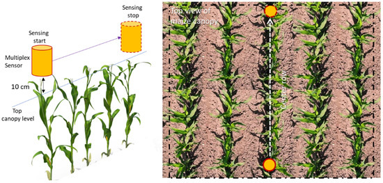
Figure 1.
Schematic view of the mobile acquisition mode of Multiplex sensor over maize canopy.
Canopy-based fluorescence measurements also consider non-vegetative objects (background soil) and other noises. To compensate for non-vegetative and saturated signals, characteristics of the far-red fluorescence induced by red (FRF_R) was used. In general, the FRF_R generates two crests of voltage at 0–20 mV and above 100mV. Hence, a threshold at 20 mV was set, and the readings with values less than threshold at FRF_R were discarded from the data set. Additionally, a filtering was necessary for the fluorescence measurement acquired on the plant to compensate for system noises. Such noises are random and constitute unwanted fluctuations that interfere with the signal. Considering that each channel (12 signals in Multiplex®3) is independent, wavelet-transformation-based denoising was applied [59]. Signal denoising was performed on fluorescence data collected for each study plot individually. Subsequently, outliers from the data were removed using the Interquartile Range (IQR) method [60]. These data filtering steps were performed using Python libraries (https://github.com/PrecisionAgLab-KSU/Fluorescence_maize (accessed on 10 September 2022)).
2.5. Vegetation Indices
In terms of plant fluorescence, chlorophyll and polyphenolic compounds (e.g., flavonols) are especially susceptible to plant N concentration [34,42,61]. Considering differential fluorescence emissions at several induction channels, chlorophyll and flavonol present in leaf tissue can be estimated [34,62]. Contrasting behavior of flavonols with N variability is observed in comparison with chlorophyll. For instance, flavonol content increases under N deficiency, while a drop in chlorophyll content is observed [63]. Hence, several vegetation indices can be sensitive to plant N content as compared with single channel fluorescence [64,65,66].
Following prior studies [39,42], seven fluorescence indices were exploited for current work. These includes four N balance indices (NBI_R, NBI_B, NBI_B, and NBI1), one flavonoid index (FLAV), and two chlorophyll indices (CHL and CHL1). Definitions and expressions of these fluorescence indices are presented in Table 1. These indices were generated from the denoised fluorescence signals.

Table 1.
Fluorescence-based vegetation indices derived from Multiplex measurements.
2.6. Statistical Analysis
Each fluorescence-based vegetation index was subjected to analysis of variance (ANOVA) to assess significant differences (at significance levels α = 0.01 and 0.05) at the V6 and V9 growth stages of maize independently. Along with a significant difference, a Tukey’s HSD test was applied to compare mean values for each N treatment at the p < 0.05 significance level. Instead of mean values of vegetation indices (over a plot), all measurements (taken in continuous mode of Multiplex sensor) over a certain treatment plot were used for the analysis. The ANOVA and Tukey’s HSD (α = 0.05) test were used to detect differences in fluorescence indices (measured using Multiplex sensor) among treatments of N. The N rates of application were set as factors to be tested with ANOVA. Fluorescence indices derived at the individual growth stages under different N rate treatments (5 N treatments at ARDEC and 6 N treatments at Iliff) were used to assess the response of fluorescence measurements acquired in mobile mode at various application rates of N fertilizer.
2.7. Estimation of Crop N Status Indicators from Fluorescence Data
The fluorescence-based vegetation indices were adopted for estimation of crop N indicators (i.e., above-ground biomass and N concentration (%)) using a machine learning regression technique. Considering the complexity of multi-channel fluorescence readings taken at the canopy scale in-motion, the ML-based regression algorithms have the potential to rapidly analyze the intricate and complex fluorescence data and extract major attributes to estimate crop N. Recent studies have shown that ML methods such as partial least square regression (PLSR), stepwise multiple linear regression (SMLR), support vector regression (SVR), and artificial neural networks (ANN) can efficiently estimate crop N content using reflectance spectroscopy [50,67,68]. Among these methods, the SVR model possess superior generalization capacity [69]. SVR can also provide a globally optimal solution to optimization problem, while the problems of local minima impede other contemporary approaches, such as neural networks. SVRs can also solve non-linear problems using Kernel methods [70,71].
Support Vector Machine (SVM) was utilized for these regression-based estimation problems to develop continuous-valued mapping functions [72]. The Support Vector Regression (SVR) technique was employed successfully in a variety of applications with remote and proximal sensors applications, including estimation of crop traits and phenological parameters [70,71,73,74]. The SVR governs a function by mapping the input feature x to target feature y which belongs to the real number space . In practice, the SVR technique is utilized to fit a nonlinear regression into a high-dimensional feature space (φ(xi)) (Figure 2) and Equation (1) as:
where regressor and bias are presented by w and b, respectively. The kernel functions (Gaussian radial basis function or polynomial functions) are often used to transform the data into a higher-dimensional feature space φ(xi) to make it possible to perform the linear fitting. SVR implements the -insensitive loss function [75] for penalizing estimates that are beyond than from the anticipated output. The value of controls the width of tube (Figure 2).
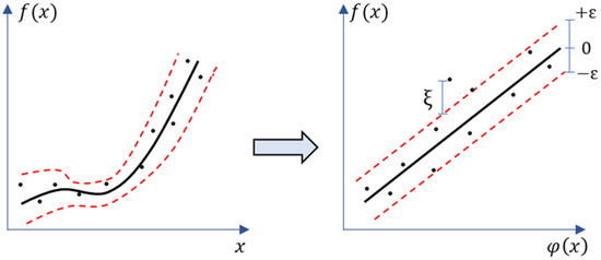
Figure 2.
Mapping a non-linear support vector regression into feature space and its ε-insensitive loss.
To cope with some infeasible constraints of the minimization problem, the ‘soft margin’ analogy was introduced by the non-negative slack variables . These slack variables quantify the deviation of the training points present outside the -zone. Subsequently, the minimization problem can be expressed as Equation (2):
where C indicates a penalty factor and, in combination with , they determine generalization capability of SVR. In addition, a kernel parameter γ is often introduced in the Gaussian radial basis function while transforming the data into φ(xi) space.
In the case of estimating plant N status indicators from fluorescence indices, the SVR model was trained using all the vegetation indices as inputs and the corresponding plant N indicator (e.g., %N) as the response. It is important to note that fluorescence indices collected in a continuous mode over a certain plot were averaged, and the mean value was used to represent the plot for the estimation problem. Hence, the total samples for each growth stages were 60 and 24 at the ARDEC and Iliff sites, respectively.
The tuned hyper-parameters of SVR, i.e., C and γ, were found by a k-fold cross-validation technique. The sample data were divided with a 60:40 ratio for training and testing. Both the training and test data were used for estimating accuracies in terms of correlation coefficient (r), and error metrics, i.e., Root Mean Square Error (RMSE) and Mean Absolute Error (MAE). Training and test accuracies were assessed for the ARDEC and Iliff sites distinctly to evaluate site-independent validation. The model prediction accuracies at the V6 and V9 growth stages were assessed to find model performances at early growth stages.
3. Results and Discussions
3.1. Discerning Variability of N Content in Crop Canopy
The sensitivity of fluorescence indices is presented with different N application rates over experimental plots of the ARDEC site in Figure 3 and Figure 4 for the V6 and V9 growth stages, respectively. For statistical analysis, data sets over two growth stages of maize were tested independently. The NBI measured from red and green induction (NBI_R and NBI_G) was successful in discriminating variability in N treatment at both growth stages. However, the discrimination was better at the V6 stage (significantly different with α = 0.05).
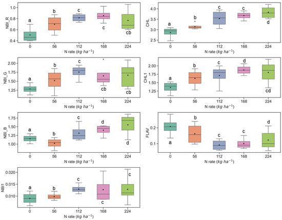
Figure 3.
Response of Multiplex fluorescence indices over maize canopy treated with different N application rates at V6 growth stage at the ARDEC site. Different letters (a, b, c, d) designate significant differences according to the Tukey’s HSD test at p < 0.05 significance level.
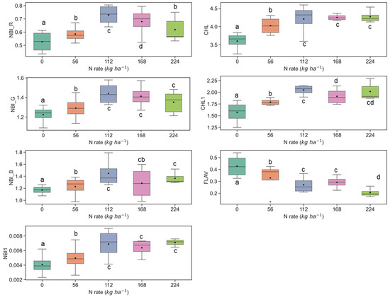
Figure 4.
Response of Multiplex fluorescence indices over maize canopy treated with different N application rates at the V9 growth stage at the ARDEC site. Different letters (a, b, c, d) designate significant differences according to the Tukey’s HSD test at p < 0.05 significance level.
The other two N balance indices (NBI_B and NBI1) indicated smaller differences in mean values along with different N treatments. In an experiment, Zhang and Tremblay [76] also highlighted that UV-induced fluorescence measurements over maize were significantly affected by N variability. The NBIs are affected by both phenolics and chlorophyll contents which are regulated by the plant N status [64,77].
The ANOVA results of Multiplex fluorescence indices showed significant effect of N treatments (Table 2). The NBI_R, NBI_G, NBI_B, NBI1, CHL, and CHL1 increased with increasing N supply, while declining tendencies were revealed for FLAV (Figure 3). However, these fluorescence indices were unresponsive to N rates of 168 kg ha−1 or above at the V6 stage. Interestingly, these indices derived at the V9 growth stages were unsuccessful in discriminating the high N rates (≥112 kg ha−1) (Figure 4). Comparatively, NBI_R indicated discrimination ability between 112 and 168 kg ha-1 treatments at the V9 stage (Figure 4), which was supported by the Tukey’s HSD test statistics. The mean values for these two samples were significantly different (as identified by two different letters in Figure 4). However, in the case of CHL, the 112 and 168 indicated similar mean values, i.e., not a significant difference in mean. The CHL1 was able to distinguish the N application rates of 112 and 168 kg ha-1 with significant mean differences. Similar discrimination capabilities were also reported by Dong et al. [44] at the V8-V12 growth stages of maize by NBI_R.
Table 2.
Analysis of variance (ANOVA) of fluorescence indices at V6 and V9 growth stages of maize as affected by different N application rates at the ARDEC and Iliff sites.
Compared with all indices, FLAV changed inversely with the N rate irrespective of growth. Accumulation of polyphenols in the leaf epidermis layer under deficiency of N can likely lead to such opposite drift of FLAV, which was contrary to the tendency of CHL and CHL1 [63,78]. On the contrary, NBIs are influenced by both chlorophylls and flavonoids present in the crop canopy and has a wide response range [42,79].
Similar results were also observed at the Iliff test site (Figure 5 and Figure 6), and they were in line with the ARDEC site data at the V6 and V9 stages. In several cases, the fluorescence indices could not differentiate among N rates which were above 135 kg ha−1 (Figure 5 and Figure 6). Comparable insensitivity of Multiplex fluorescence response to high N rates has been also reported in other studies [42,44,66].
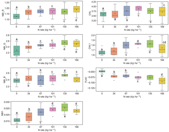
Figure 5.
Response of Multiplex fluorescence indices over maize canopy treated with different N application rates at the V6 growth stage at the Iliff site. Different letters (a, b, c, d, e) indicate significant differences according to the Tukey’s HSD test at p < 0.05 significance level.
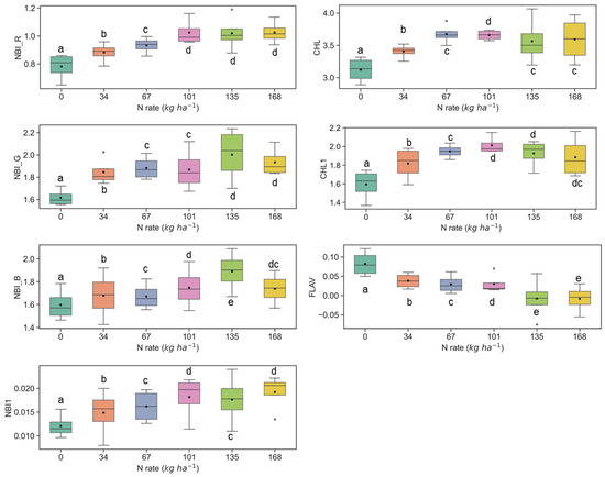
Figure 6.
Response of Multiplex fluorescence indices over maize canopy treated with different N application rates at the V9 growth stage at the Iliff site. Different letters (a, b, c, d, e) indicate significant differences according to the Tukey’s HSD test at p < 0.05 significance level.
3.2. Accuracy Assessment of Crop Canopy N Indicators Estimated Using Machine Learning Model
The seven fluorescence indices were further utilized for quantitative assessment of maize N status from the V6 and V9 stages. Each individual fluorescence-based vegetation index was used to train the SVR model for the V6 and V9 stages. Accuracies in both the train and test data for prediction of plant nitrogen concentration (%N) and biomass are presented on a 1:1 plot (Figure 7).
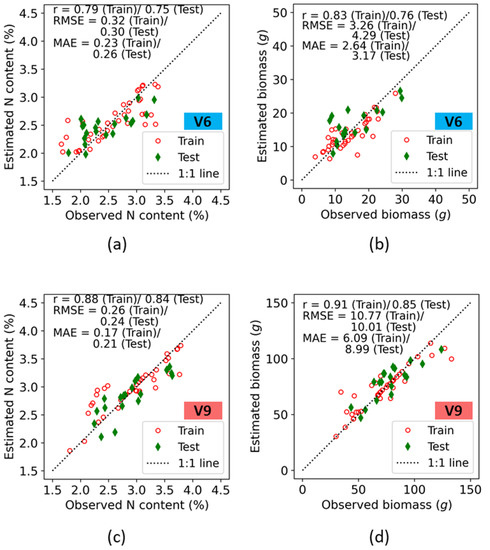
Figure 7.
Training and test accuracies of crop N indicators retrieval using fluorescence indices at the V6 (a,b), and V9 (c,d) growth stages of maize at the ARDEC site.
Irrespective of growth stages, among the various values of the two N indicators observed (i.e., biomass, and N concentration), the best correlation coefficient for the relationship between the observed and the predicted values was exhibited by the biomass (r = 0.83 (Train)/0.76 (Test) at V6, and 0.91 (Train)/0.85 (Test) at V9). At the V6 growth stage, the error estimates for N concentration showed an RMSE of 0.32 (Train)/0.30 (Test) and MAE of 0.23 (Train)/0.26 (Test), with the estimates following the 1:1 line. However, at lower N concentration ranges, overestimation was observed in both the train and test results. This deviation may be associated with background soil effects on the fluorescence measurements at lower N% (lower biomass at the V6 stage). For the biomass, the error estimates were comparatively higher. The RMSE values for biomass were 3.26 and 4.29 for the train and test data, respectively, which were within 15–18% of their respective sample mean values ( in the observed data.
It was expected that, when comparing growth stages, higher estimation accuracies would occur at the V9 stages because the crop is further developed and plants are taller with wider leaf blades, thus contributing to more interception area for fluorescence measurements when compared with the V6 growth stage. This leads to a higher dynamic range of plant N indicators at V9 than at V6. Hence, the sample mean values of observed parameters had a higher range. For the %N, the RMSE values of both the train and test datasets were less than 10% of the ranges of their means (). The error estimates for biomass indicated that RMSE was 10.77 (Train)/10.01 (Test) and MAE was 6.09 (Train)/8.99 (Test), with the estimates following the 1:1 line.
Accuracies in both the train and test data for prediction of plant nitrogen concentration (%N) and biomass at the Iliff site are presented on a 1:1 plot (Figure 8). As at the ARDEC site, the best correlation coefficient was observed for biomass predictions at both the V6 and V9 growth stages, with an r value of 0.76 (Train)/0.71 (Test) at V6, and an r value of 0.96 (Train)/0.94 (Test) at V9. At the V6 stage, the %N plot indicated a higher estimated error. The RMSE values for %N were 0.17 and 0.27 for the train and test data, respectively, which is within 5–7% of their respective sample mean values ( in observed data. However, an underestimation from the 1:1 line was observed throughout the entire range of %N for the train and test data. The biomass followed the 1:1 line for the entire ranges.
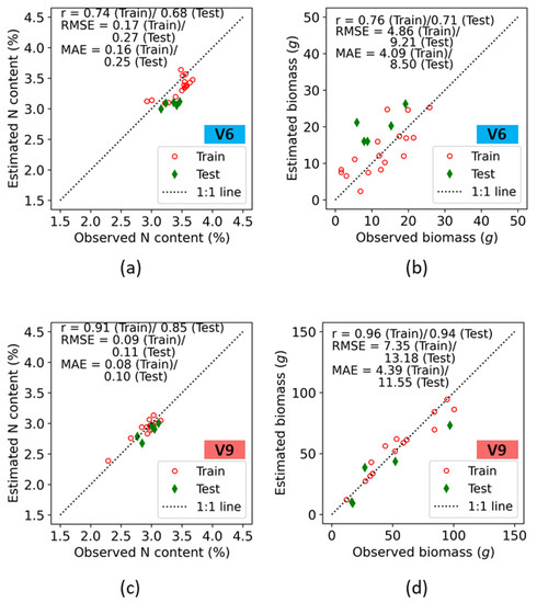
Figure 8.
Training and test accuracies of crop N indicators retrieval using fluorescence indices at the V6 (a,b), and V9 (c,d) growth stages of maize at the Iliff site.
Crop parameter estimates at the V9 growth stage indicated higher values of r as compared with V6 growth stage. The r values across the two crop parameters were 0.91 (Train)/0.85 (Test), and 0.96 (Train)/0.94 (Test) for %N and biomass, respectively. For both N indicators, the RMSE values at train and test were < 10% of the ranges of their means. Best results were obtained for the biomass, and its error estimates resulted in an RMSE of 7.35 (Train)/13.18 (Test) and a MAE of 4.39 (Train)/11.55 (Test), with the estimates following the 1:1 line.
4. Discussion
The mobile fluorescence measurements at the V6 and V9 growth stages indicated that it can distinguish the variability of N concentration in plant canopy at early growth stages. However, the differential sensitivity of fluorescence measurements at the V6 and V9 growth stages (Figure 3, Figure 4, Figure 5 and Figure 6) can be attributed to the variations of N uptake rates at these periods. The advancement from V6 to V9 led to more leaves unfolding and being exposed to sunlight, which increased the rate of dry matter accumulation. However, upon attaining the optimal N level, the N concentration in plants did not alter significantly [37]. Even though more N was available in the soil from N fertilizer, plants did not uptake additional N. It can be also observed in Figure 9 and Figure 10 that the plant nitrogen concentrations (%N) were almost the same among treatment plots with higher N application rate (i.e., 135 and 168 kg ha−1 at the Iliff site during both the V6 and V9 stages, respectively). This showed undistinguished variation of the fluorescence indices with higher N rates for both the V6 and V9 growth stages at the ARDEC and Iliff sites. The N status (%N and biomass) was also responsive to the different N treatments (Figure 9 and Figure 10). This demonstrated the effectiveness of the treatments imposed on maize crop to produce a range of N variability. Such a wide range helps while training a machine learning model.
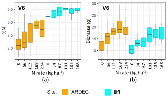
Figure 9.
Variability of %N (a), and biomass (b) with different N rate applications at V6 growth stage of maize for two sites.
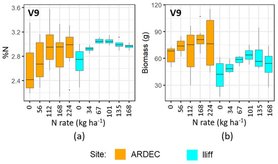
Figure 10.
Variability of %N (a) and biomass (b) with different N rate applications at V9 growth stage of maize for two sites.
From a previous study over the same experiment site by Siqueira [52], it was reported that NDVI values measured with a GreenSeeker sensor indicated a significant (α = 0.05) increase from one growth stage to the other (V4 to V8 stages of maize). However, NDVI was not able to distinguish among N treatments throughout these growth stages. There was a significant variability in NDVI across growth stages, but this variability did not follow a positive correlation with the N rates applied to the plots. On the other hand, the fluorescence indices in this current study showed variability with different treatments at the V6 and V9 stages. It is evident from Figure 3 to Figure 6 that fluorescence indices better discriminate N treatment effects. Similar discrimination capabilities were also reported by Dong et al. [44] at V8–V12 growth stages of maize by fluorescence indices.
Another interesting point to note is that although there are plant population differences within different plots over two sites (ARDEC and Iliff), it does not affect the final fluorescence measurement used for the analysis. This can be explained by the signal processing step (Section 2.4) where the raw data acquired through Multiplex sensor underwent two major signal processing steps: (a) compensation for non-vegetative/saturated signals and (b) signal denoising with wavelet transformation. For example, a raw signal at FRF_G channel is presented in Figure 11a in the time domain. In the frequency domain (Figure 11b), the main signal indicates higher amplitude values, while signal amplitude values <10 unit are possibly noise as they have lower occurrence than the original signal. Subsequently, using a predefined threshold value, those noisy signals were removed, and the data were again transformed back from the frequency domain to the time domain to get a denoised signal (Figure 11c,d). Hence, if there is low plant density within a row, the signal processing step takes care of eliminating such signal (possibly from non-vegetative part).
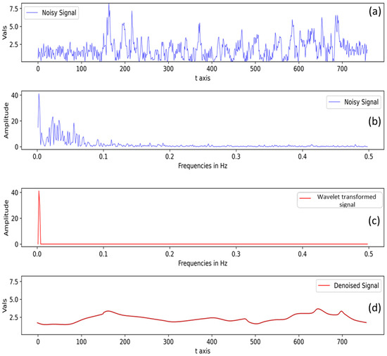
Figure 11.
Processed signal after non-vegetative signal compensation (a) signal in time domain and (b) signal in frequency domain. Signal denoising with wavelet-transformation-denoised (c) signal in frequency domain, and (d) denoised signal in time domain.
The estimation of crop N indicators with the SVR model training and testing accuracies indicated good accuracies for each growth stage (V6 and V9) separately, although the performances were inferior at the V6 growth stage. Dong et al. [37] also reported higher variations in plant nitrogen content estimates at V6 than at V8 stages of maize using fluorescence indices (NBI, FLAV, and CHL). As compared with the present study, the experiment by Dong et al. [37] was conducted with fluorescence measurement at the leaf-scale level. Hence, the predictions of plant nitrogen are significantly affected by the selection of leaf to be sampled. The photosynthetic photon flux density decreases with increasing canopy depth and potentially leads to preferential distribution of N to upper leaves [80]. On the contrary, the above canopy level fluorescence data considers all leaves and stem as a whole target and averages out such preferences in N distribution. Hence, the fluorescence measurements on a mobile platform or mode also provides opportunity to transfer similar methodology and evaluation for other plant types. Specifically, the diverse leaf anatomy of plants can present challenges for measurement with this instrument given the relatively small sampling area (approximately 80 cm2 of Multiplex®3). With a leaf-scale measurement, it requires defined and easily identifiable positions on leaves to standardize the measurement protocol along with appreciable repetition for representative measurement. On the other hand, for the mobile fluorescence at canopy scale, it is not restricted by finding such a standard location, and data acquisition is independent of plant type. However, the variation of N indicators derived from fluorescence measurements would vary plant to plant. Hence, distinct machine learning models are required to be trained for such a case.
Huang et al. [36] also tested the mobile sensing mode against the standard above-canopy level and leaf-scale mode for rice with Multiplex. They reported better sensitivity to N rate in fluorescence measurements when data were acquired in mobile mode. Measurements taken with leaf scale were least influenced by differential N rate. These outcomes are inconsistent with the experimental analysis reported by Diago et al. [43] studying grapevines. Diago et al. [43] described a 20% loss of information arising from mobile operation of Multiplex as compared with the above-canopy stationary mode. This is potentially due to the difference in the adaxial and abaxial side of a leaf in planophiles as compared with an erectophile (rice) plant. Similarly, Zhang et al. [76] found Multiplex measurements in leaf-scale mode from maize leaves better for distinguishing maize N status than in the above-canopy stationary mode.
The choice of the SVR model as a regression tool is based on its superior generalization capacity [69]. Generalization capability helps to compensate for the bias–variance of model predictions. This can be explained with an example from the fluorescence measurement and plant nitrogen case. For ease of visualization on a 3D plot, NBI_R and FLAV were selected as inputs to the regression model instead of all fluorescence indices. The model training was performed using plant N% data at the ARDEC site at the V9 stage. It is apparent from Figure 12 that bias and MSE in SVR model indicate the lowest values as compared to multiple linear regression (MLR) and partial least square regression (PLSR) models.
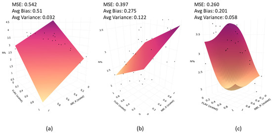
Figure 12.
Prediction plane from (a) Multiple Linear Regression; (b) Partial Least Square Regression (PLSR); and (c) Support Vector Regression (SVR). The average Mean Squared Error (MSE), bias, and variances are highlighted for each model.
Although variance increased to 0.058 as compared with MLR, this is common in bias–variance trade-off [81]. Even though PLSR produced less bias than MLR, the high variance values are evident. A similar analogy can be translated to a multi-dimensional case (considering all fluorescence indices used as input), but it is difficult to visualize the prediction surface. Unlike a flat sheet surface with MLR and PLSR, SVR allows for a more flexible surface enabling a more accurate fit to data. The superiority of the SVR model was also demonstrated in the literature on the thematic area of plant bio-geophysical traits [48,73,82]. It is noteworthy that PLSR computes linear combination of input features, but in practical scenarios, data often lie on a nonlinear manifold. On the contrary, SVR formulation considers non-linearity of data using kernel operations as introduced in Section 2.7.
In this study, fluorescence-based measurements were conducted on a mobile platform to train a machine learning model (SVR) to determine absolute sufficiency value of plant nitrogen using indicators of the crop N status. Such a quantification of N status would be useful for the prescriptive–corrective N management [83,84]. The SVR model estimates can be further used to calculate recommended N fertilizer corrections. It can allow us to develop a monitoring/application system enabling the technical capacity of such a system to spoon-feed N as required by the crop. Numerous factors can distress the fluorescence measurements acquired in a mobile continuous mode with the Multiplex system. This may include background (soil) noise, variable distance-to-target, or canopy gap fraction, which can affect the signal-to-noise ratio and generate uncertainties while estimating crop N status. For instance, Longchamps and Khosla [39] found that the fluorescence signal decreased drastically between 10 and 15 cm from the target, indicating a strong influence of distance-to-target on potential outcomes. Nevertheless, values of RMSE were within 20% of mean values while estimating %N and biomass for each growth stage (V6 and V9). The variance analysis also indicated variability in plant N indicators with differential N application rate using the mobile mode of Multiplex measurements. Additionally, the mobile mode allows the sensor to be mounted on an autonomous vehicle, which helps in large area mapping and adjusting sensor distance from the canopy to optimize the information loss. The spatial resolution of data can be further studied as an additional experiment by configuring the acquisition mechanism of the Multiplex sensor. It is essential to standardize the calibration [43] and filtering strategy (to improve the signal-to-noise ratio) in order to ensure the reliability of the fluorescence sensor measurements in the mobile mode in a precision farming context.
5. Conclusions and Perspectives
The present study focused on the potential of mobile fluorescence sensing to quantify canopy N variability in terms of %N and biomass at early growth stages (V6 and V9) of maize. The fluorescence indices were further utilized to address the estimation potential of crop N status indicators using ML model. The training and testing accuracies of ML regression were assessed while estimating %N and biomass for V6 and V9 growth stages separately over two test sites.
The ANOVA results of Multiplex fluorescence indices measured over maize canopy treated with different N rates indicated that fluorescence measurements were able to discern differences between N rates. However, entire fluorescence indices were insensitive to high N rates (>168 kg ha−1) at both the V6 and V9 growth stages. With respect to canopy N indicator estimation, independent site analysis confirmed that fluorescence indices aided with ML technique (SVR) yield reasonable accuracies at the V6 and V9 growth stages of maize, although the performances were inferior at the V6 growth stage. Both the training and test data in SVR provided high correlation coefficients and low estimation errors for predicted N status indicators at the V6 and V9 growth stages. These results provide an inference that the SVR could be an effective and robust technique for fluorescence-based crop N status indicator estimation.
Estimation of canopy N indicators can be further examined with advanced machine learning models (e.g., neural networks or the optimization frameworks (particle swarm optimization and genetic algorithms)) to test their robustness, uncertainty, and computation costs. These models can be trained with more realistic data sets. In this direction, theoretical radiative transfer models in fluorescence spectrum (SCOPE, Flourmod) could also be utilized to produce a synthetic data set in an alternative pathway which covers a varied range of conditions to avoid limitations associated with the site-dependent data. Another limitation of this study is the local adjustment of the model in a rather homogeneous region. Further investigation should, therefore, analyze the robustness of the method over heterogeneous agricultural regions and beyond. Additionally, a larger scale approach—involving more heterogeneous soil, row spacing, water deficit conditions, and crop stress—needs to be taken into account, as these factors might influence the fluorescence measurements at early growth stages of maize.
Author Contributions
Conceptualization and supervision, R.K.; project administration, R.K. and L.L.; methodology, R.S., L.L. and D.M.; data curation, R.S.; investigation, R.S. and L.L.; formal analysis, R.S. and D.M.; software and code, D.M.; writing—original draft, R.S. and D.M.; writing—review and editing, D.M., L.L. and R.K.; visualization, D.M.; resources and funding acquisition, R.K. All authors have read and agreed to the published version of the manuscript.
Funding
Funding of this project was partially provided by Colorado State University Agricultural Experiment Station in partnership with Force-A, and multiple on-going research support funding.
Institutional Review Board Statement
Not applicable.
Informed Consent Statement
Not applicable.
Data Availability Statement
The data presented in this study are available on request from the corresponding author.
Conflicts of Interest
The authors declare no conflict of interest.
Code Availability
Code for fluorescence data cleaning and regression analysis is provided in Github repository and can be accessed from the following link. https://github.com/PrecisionAgLab-KSU/Fluorescence_maize (accessed on 8 September 2022).
References
- Gupta, M.L.; Khosla, R. Precision nitrogen management and global nitrogen use efficiency. In Proceedings of the 11th International Conference on Precision Agriculture, Indianapolis, IN, USA, 15–18 July 2012. [Google Scholar]
- Khosla, R.; Shaver, T. Zoning in on nitrogen needs. Colo. State Univ. Agron. Newsl. 2001, 21, 24–26. [Google Scholar]
- Cordero, E.; Longchamps, L.; Khosla, R.; Sacco, D. Spatial management strategies for nitrogen in maize production based on soil and crop data. Sci. Total Environ. 2019, 697, 133854. [Google Scholar] [CrossRef]
- Stafford, J.V. Implementing Precision Agriculture in the 21st Century. J. Agric. Eng. Res. 2000, 76, 267–275. [Google Scholar] [CrossRef]
- Koch, B.; Khosla, R.; Frasier, W.M.; Westfall, D.G.; Inman, D. Economic feasibility of variable-rate nitrogen application utilizing site-specific management zones. Agron. J. 2004, 96, 1572–1580. [Google Scholar] [CrossRef]
- Muñoz-Huerta, R.F.; Guevara-Gonzalez, R.G.; Contreras-Medina, L.M.; Torres-Pacheco, I.; Prado-Olivarez, J.; Ocampo-Velazquez, R.V. A Review of Methods for Sensing the Nitrogen Status in Plants: Advantages, Disadvantages and Recent Advances. Sensors 2013, 13, 10823–10843. [Google Scholar] [CrossRef]
- Colaço, A.F.; Bramley, R.G.V. Do crop sensors promote improved nitrogen management in grain crops? Field Crops Res. 2018, 218, 126–140. [Google Scholar] [CrossRef]
- Antille, D.L.; Lobsey, C.R.; McCarthy, C.L.; Thomasson, J.A.; Baillie, C.P. A review of the state of the art in agricultural automation. Part IV: Sensor-based nitrogen management technologies. In 2018 ASABE Annual International Meeting; American Society of Agricultural and Biological Engineers: St. Joseph, MI, USA, 2018; p. 1. [Google Scholar]
- Corti, M.; Cavalli, D.; Cabassi, G.; Gallina, P.M.; Bechini, L. Does remote and proximal optical sensing successfully estimate maize variables? A review. Eur. J. Agron. 2018, 99, 37–50. [Google Scholar] [CrossRef]
- Mulla, D.J.; Miao, Y. Precision Farming. In Land Resources Monitoring, Modeling, and Mapping with Remote Sensing; Thenkabail, P.S., Ed.; CRC Press: Boca Raton, FL, USA, 2016. [Google Scholar]
- Ali, M.M.; Al-Ani, A.; Eamus, D.; Tan, D.K.Y. Leaf nitrogen determination using non-destructive techniques–A review. J. Plant Nutr. 2017, 40, 928–953. [Google Scholar] [CrossRef]
- Malenovský, Z.; Mishra, K.B.; Zemek, F.; Rascher, U.; Nedbal, L. Scientific and technical challenges in remote sensing of plant canopy reflectance and fluorescence. J. Exp. Bot. 2009, 60, 2987–3004. [Google Scholar] [CrossRef] [PubMed]
- Berger, K.; Verrelst, J.; Féret, J.B.; Wang, Z.; Wocher, M.; Strathmann, M.; Danner, M.; Mauser, W.; Hank, T. Crop nitrogen monitoring: Recent progress and principal developments in the context of imaging spectroscopy missions. Remote Sens. Environ. 2020, 242, 111758. [Google Scholar] [CrossRef]
- Li, H.; Zhao, C.; Huang, W.; Yang, G. Non-uniform vertical nitrogen distribution within plant canopy and its estimation by remote sensing: A review. Field Crops Res. 2013, 142, 75–84. [Google Scholar] [CrossRef]
- Shaver, T.M.; Khosla, R.; Westfall, D.G. Evaluation of two crop canopy sensors for nitrogen variability determination in irrigated maize. Precis. Agric. 2011, 12, 892–904. [Google Scholar] [CrossRef]
- Schepers, J.S.; Blackmer, T.M.; Wilhelm, W.W.; Resende, M. Transmittance and Reflectance Measurements of Corn Leaves from Plants with Different Nitrogen and Water Supply. J. Plant Physiol. 1996, 148, 523–529. [Google Scholar] [CrossRef]
- Ercoli, L.; Mariotti, M.; Masoni, A.; Massantini, F. Relationship between nitrogen and chlorophyll content and spectral properties in maize leaves. Eur. J. Agron. 1993, 2, 113–117. [Google Scholar] [CrossRef]
- Haboudane, D.; Miller, J.R.; Tremblay, N.; Zarco-Tejada, P.J.; Dextraze, L. Integrated narrow-band vegetation indices for prediction of crop chlorophyll content for application to precision agriculture. Remote Sens. Environ. 2002, 81, 416–426. [Google Scholar] [CrossRef]
- Gitelson, A.A.; Gritz, Y.; Merzlyak, M.N. Relationships between leaf chlorophyll content and spectral reflectance and algorithms for non-destructive chlorophyll assessment in higher plant leaves. J. Plant Physiol. 2003, 160, 271–282. [Google Scholar] [CrossRef] [PubMed]
- Heege, H.J.; Reusch, S.; Thiessen, E. Prospects and results for optical systems for site-specific on-the-go control of nitro-gen-top-dressing in Germany. Precis. Agric. 2008, 9, 115–131. [Google Scholar] [CrossRef]
- Homolová, L.; Malenovský, Z.; Clevers, J.G.; García-Santos, G.; Schaepman, M. Review of optical-based remote sensing for plant trait mapping. Ecol. Complex. 2013, 15, 1–16. [Google Scholar] [CrossRef]
- Inman, D.; Khosla, R.; Reich, R.M.; Westfall, D.G. Active remote sensing and grain yield in irrigated maize. Precis. Agric. 2007, 8, 241–252. [Google Scholar] [CrossRef]
- Teal, R.K.; Tubana, B.; Girma, K.; Freeman, K.W.; Arnall, D.B.; Walsh, O.; Raun, W.R. In-season prediction of corn grain yield potential using normalized difference vegetation index. Agron. J. 2006, 98, 1488–1494. [Google Scholar] [CrossRef]
- Cao, Q.; Miao, Y.; Shen, J.; Yu, W.; Yuan, F.; Cheng, S.; Huang, S.; Wang, H.; Yang, W.; Liu, F. Improving in-season estimation of rice yield potential and responsiveness to topdressing nitrogen application with Crop Circle active crop canopy sensor. Precis. Agric. 2016, 17, 136–154. [Google Scholar] [CrossRef]
- Inman, D.; Khosla, R.; Mayfield, T. On-the-go active remote sensing for efficient crop nitrogen management. Sens. Rev. 2005, 25, 209–214. [Google Scholar] [CrossRef]
- Naser, M.; Khosla, R.; Longchamps, L.; Dahal, S. Using NDVI to Differentiate Wheat Genotypes Productivity Under Dryland and Irrigated Conditions. Remote Sens. 2020, 12, 824. [Google Scholar] [CrossRef]
- Yao, Y.; Miao, Y.; Huang, S.; Gao, L.; Ma, X.; Zhao, G.; Jiang, R.; Chen, X.; Zhang, F.; Yu, K.; et al. Active canopy sensor-based precision N management strategy for rice. Agron. Sustain. Dev. 2012, 32, 925–933. [Google Scholar] [CrossRef]
- Olfs, H.W.; Blankenau, K.; Brentrup, F.; Jasper, J.; Link, A.; Lammel, J. Soil-and plant-based nitrogen-fertilizer recommendations in arable farming. J. Soil Sci. Plant Nutr. 2005, 168, 414–431. [Google Scholar] [CrossRef]
- Bredemeier, C.; Schmidhalter, U. Laser-induced chlorophyll fluorescence sensing to determine biomass and nitrogen uptake of winter wheat under controlled environment and field condition. In Proceedings of the 5th European Conference on Precision Agriculture, Uppsala, Sweden, 9–12 June 2005; Wageningen Academic Publishers: Wageningen, The Netherlands, 2005; pp. 273–280. [Google Scholar]
- McMurtrey, J.E., III; Chappelle, E.W.; Kim, M.S.; Meisinger, J.J.; Corp, L.A. Distinguishing nitrogen fertilization levels in field corn (Zea mays L.) with actively induced fluorescence and passive reflectance measurements. Remote Sens. Environ. 1994, 47, 36–44. [Google Scholar] [CrossRef]
- Maxwell, K.; Johnson, G.N. Chlorophyll fluorescence—A practical guide. J. Exp. Bot. 2000, 51, 659–668. [Google Scholar] [CrossRef]
- Burchard, P.; Bilger, W.; Weissenböck, G. Contribution of hydroxycinnamates and flavonoids to epi-dermal shielding of UV-A and UV-B radiation in developing rye primary leaves as assessed by ultraviolet-induced chlorophyll fluorescence measurements. Plant Cell Environ. 2000, 23, 1373–1380. [Google Scholar] [CrossRef]
- Bilger, W.; Johnsen, T.; Schreiber, U. UV-excited chlorophyll fluorescence as a tool for the assessment of UV-protection by the epidermis of plants. J. Exp. Bot. 2001, 52, 2007–2014. [Google Scholar] [CrossRef]
- Tremblay, N.; Wang, Z.; Cerovic, Z.G. Sensing crop nitrogen status with fluorescence indicators. A review. Agron. Sustain. Dev. 2012, 32, 451–464. [Google Scholar] [CrossRef]
- Li, J.W.; Zhang, J.X.; Zhao, Z.; Lei, X.D.; Xu, X.L.; Lu, X.X.; Weng, D.L.; Gao, Y.; Cao, L.K. Use of fluorescence-based sensors to determine the nitrogen status of paddy rice. J. Agric. Sci. 2013, 151, 862–871. [Google Scholar] [CrossRef]
- Huang, S.; Miao, Y.; Yuan, F.; Cao, Q.; Ye, H.; Lenz-Wiedemann, V.I.; Bareth, G. In-Season Diagnosis of Rice Nitrogen Status Using Proximal Fluorescence Canopy Sensor at Different Growth Stages. Remote Sens. 2019, 11, 1847. [Google Scholar] [CrossRef]
- Dong, R.; Miao, Y.; Wang, X.; Chen, Z.; Yuan, F.; Zhang, W.; Li, H. Estimating plant nitrogen concentration of maize using a leaf fluorescence sensor across growth stages. Remote Sens. 2020, 12, 1139. [Google Scholar] [CrossRef]
- de Souza, R.; Peña-Fleitas, M.T.; Thompson, R.B.; Gallardo, M.; Grasso, R.; Padilla, F.M. Use of fluorescence indices as predictors of crop N status and yield for greenhouse sweet pepper crops. Precis. Agric. 2022, 23, 278–299. [Google Scholar] [CrossRef]
- Longchamps, L.; Khosla, R. Early Detection of Nitrogen Variability in Maize Using Fluorescence. Agron. J. 2014, 106, 511–518. [Google Scholar] [CrossRef]
- Martin, K.L.; Girma, K.; Freeman, K.W.; Teal, R.K.; Tubańa, B.; Arnall, D.B.; Chung, B.; Walsh, O.; Solie, J.B.; Stone, M.L.; et al. Expression of Variability in Corn as Influenced by Growth Stage Using Optical Sensor Measurements. Agron. J. 2007, 99, 384–389. [Google Scholar] [CrossRef]
- Siqueira, R.; Longchamps, L.; Dahal, S.; Khosla, R. Use of Fluorescence Sensing to Detect Nitrogen and Potassium Variability in Maize. Remote Sens. 2020, 12, 1752. [Google Scholar] [CrossRef]
- Agati, G.; Foschi, L.; Grossi, N.; Guglielminetti, L.; Cerovic, Z.G.; Volterrani, M. Fluorescence-based versus reflectance proximal sensing of nitrogen content in Paspalum vaginatum and Zoysia matrella turfgrasses. Eur. J. Agron. 2013, 45, 39–51. [Google Scholar] [CrossRef]
- Diago, M.P.; Rey-Carames, C.; Le Moigne, M.; Fadaili, E.M.; Tardáguila, J.; Cerovic, Z.G. Calibration of non-invasive fluorescence-based sensors for the manual and on-the-go assessment of grapevine vegetative status in the field. Aust. J. Grape Wine Res. 2016, 22, 438–449. [Google Scholar] [CrossRef]
- Dong, R.; Miao, Y.; Wang, X.; Yuan, F.; Kusnierek, K. Canopy Fluorescence Sensing for In-Season Maize Nitrogen Status Diagnosis. Remote Sens. 2021, 13, 5141. [Google Scholar] [CrossRef]
- Monici, M. Cell and tissue autofluorescence research and diagnostic applications. Biotechnol. Annu. Rev. 2005, 11, 227–256. [Google Scholar] [CrossRef] [PubMed]
- Luisier, F.; Vonesch, C.; Blu, T.; Unser, M. Fast interscale wavelet denoising of Poisson-corrupted images. Signal Process. 2010, 90, 415–427. [Google Scholar] [CrossRef]
- Yao, X.; Huang, Y.; Shang, G.; Zhou, C.; Cheng, T.; Tian, Y.; Cao, W.; Zhu, Y. Evaluation of Six Algorithms to Monitor Wheat Leaf Nitrogen Concentration. Remote Sens. 2015, 7, 14939–14966. [Google Scholar] [CrossRef]
- Chlingaryan, A.; Sukkarieh, S.; Whelan, B. Machine learning approaches for crop yield prediction and nitrogen status estimation in precision agriculture: A review. Comput. Electron. Agric. 2018, 151, 61–69. [Google Scholar] [CrossRef]
- Berger, K.; Verrelst, J.; Féret, J.-B.; Hank, T.; Wocher, M.; Mauser, W.; Camps-Valls, G. Retrieval of aboveground crop nitrogen content with a hybrid machine learning method. Int. J. Appl. Earth Obs. Geoinf. 2020, 92, 102174. [Google Scholar] [CrossRef]
- Wang, X.; Miao, Y.; Dong, R.; Zha, H.; Xia, T.; Chen, Z.; Kusnierek, K.; Mi, G.; Sun, H.; Li, M. Machine learning-based in-season nitrogen status diagnosis and side-dress nitrogen recommendation for corn. Eur. J. Agron. 2021, 123, 126193. [Google Scholar] [CrossRef]
- Soil Survey Staff, Natural Resources Conservation Service, United States Department of Agriculture, Web Soil Survey. Available online: https://websoilsurvey.sc.egov.usda.gov (accessed on 20 May 2012).
- Siqueira, R.T.T. Characterizing Nitrogen Deficiency of Maize at Early Growth Stages Using Fluorescence Measurements. Ph.D. Thesis, Colorado State University, Fort Collins, CO, USA, 2015. Available online: http://hdl.handle.net/10217/173445 (accessed on 8 September 2022).
- Davis, J.G.; Westfall, D.G. Fertilizing Corn. Colorado State University Extension Fact Sheet No. 0.538. 2009. Available online: https://extension.colostate.edu/docs/pubs/crops/00538.pdf (accessed on 8 September 2022).
- Ritchie, S.W.; Hanway, J.J.; Benson, G.O.; Herman, J.C. How a Corn Plant Develops: Special Report No 48; Iowa State University of Science and Technology Cooperative Extension Service: Ames, IA, USA, 1997. [Google Scholar]
- Bilger, W.; Veit, M.; Schreiber, L.; Schreiber, U. Measurement of leaf epidermal transmittance of UV radiation by chlorophyll fluorescence. Physiol. Plant. 1997, 101, 754–763. [Google Scholar] [CrossRef]
- Cerovic, Z.G.; Ounis, A.; Cartelat, A.; Latouche, G.; Goulas, Y.; Meyer, S.; Moya, I. The use of chlorophyll fluorescence excitation spectra for the non-destructive in situ assessment of UV-absorbing compounds in leaves. Plant Cell Environ. 2002, 25, 1663–1676. [Google Scholar] [CrossRef]
- Agati, G.; Meyer, S.; Matteini, P.; Cerovic, Z.G. Assessment of Anthocyanins in Grape (Vitis vinifera L.) Berries Using a Noninvasive Chlorophyll Fluorescence Method. J. Agric. Food Chem. 2007, 55, 1053–1061. [Google Scholar] [CrossRef]
- Sawyer, J.; Nafziger, E.; Randall, G.; Bundy, L.; Rehm, G.; Joern, B. Concepts and Rationale for Regional Nitrogen Rate Guidelines for Corn; Iowa State University-University Extension: Ames, IA, USA, 2006; p. 28. [Google Scholar]
- Lee, G.; Gommers, R.; Waselewski, F.; Wohlfahrt, K.; O’Leary, A. PyWavelets: A Python package for wavelet analysis. J. Open Source Softw. 2019, 4, 1237. [Google Scholar] [CrossRef]
- Barbato, G.; Barini, E.M.; Genta, G.; Levi, R. Features and performance of some outlier detection methods. J. Appl. Stat. 2011, 38, 2133–2149. [Google Scholar] [CrossRef]
- Fox, R.H.; Walthall, C.L. Crop monitoring technologies to assess nitrogen status. In Nitrogen in Agricultural Systems, Agronomy Monograph No. 49; Schepers, J.S., Raun, W.R., Eds.; American Society of Agronomy, Crop Science Society of America, Soil Science Society of America: Madison, WI, USA, 2008; pp. 647–674. [Google Scholar]
- Padilla, F.M.; Gallardo, M.; Peña-Fleitas, M.T.; de Souza, R.; Thompson, R.B. Proximal Optical Sensors for Nitrogen Management of Vegetable Crops: A Review. Sensors 2018, 18, 2083. [Google Scholar] [CrossRef] [PubMed]
- Bragazza, L.; Freeman, C. High nitrogen availability reduces polyphenol content in Sphagnum peat. Sci. Total Environ. 2007, 377, 439–443. [Google Scholar] [CrossRef] [PubMed]
- Cartelat, A.; Cerovic, Z.; Goulas, Y.; Meyer, S.; Lelarge, C.; Prioul, J.-L.; Barbottin, A.; Jeuffroy, M.-H.; Gate, P.; Agati, G.; et al. Optically assessed contents of leaf polyphenolics and chlorophyll as indicators of nitrogen deficiency in wheat (Triticum aestivum L.). Field Crop. Res. 2005, 91, 35–49. [Google Scholar] [CrossRef]
- Samborski, S.M.; Tremblay, N.; Fallon, E. Strategies to make use of plant sensors-based diagnostic in-formation for nitrogen recommendations. Agron. J. 2009, 101, 800–816. [Google Scholar] [CrossRef]
- Padilla, F.M.; Peña-Fleitas, M.T.; Gallardo, M.; Thompson, R.B. Proximal optical sensing of cucumber crop N status using chlorophyll fuorescence indices. Eur. J. Agron. 2016, 73, 83–97. [Google Scholar] [CrossRef]
- Karimi, Y.; Prasher, S.; Patel, R.; Kim, S. Application of support vector machine technology for weed and nitrogen stress detection in corn. Comput. Electron. Agric. 2006, 51, 99–109. [Google Scholar] [CrossRef]
- Ecarnot, M.; Compan, F.; Roumet, P. Assessing leaf nitrogen content and leaf mass per unit area of wheat in the field throughout plant cycle with a portable spectrometer. Field Crop. Res. 2013, 140, 44–50. [Google Scholar] [CrossRef]
- Behzad, M.; Asghari, K.; Eazi, M.; Palhang, M. Generalization performance of support vector machines and neural networks in runoff modeling. Expert Syst. Appl. 2009, 36, 7624–7629. [Google Scholar] [CrossRef]
- Durbha, S.S.; King, R.L.; Younan, N.H. Support vector machines regression for retrieval of leaf area index from multiangle imaging spectroradiometer. Remote Sens. Environ. 2007, 107, 348–361. [Google Scholar] [CrossRef]
- Mountrakis, G.; Im, J.; Ogole, C. Support vector machines in remote sensing: A review. ISPRS J. Photogramm. Remote Sens. 2011, 66, 247–259. [Google Scholar] [CrossRef]
- Vapnik, V. The Nature of Statistical Learning Theory; Springer: Berlin/Heidelberg, Germany, 2013. [Google Scholar]
- Camps-Valls, G.; Bruzzone, L.; Rojo-Alvarez, J.L.; Melgani, F. Robust support vector regressionfor biophysical variable estimation from remotely sensed images. IEEE Geosci. Remote Sens Lett. 2006, 3, 339–343. [Google Scholar] [CrossRef]
- Yang, J.; Gong, W.; Shi, S.; Du, L.; Sun, J.; Song, S.; Chen, B.; Zhang, Z. Analyzing the performance of fluorescence parameters in the monitoring of leaf nitrogen content of paddy rice. Sci. Rep. 2016, 6, 28787. [Google Scholar] [CrossRef]
- Smola, A.J.; Schölkopf, B. A tutorial on support vector regression. Stat Comput. 2004, 14, 199–222. [Google Scholar] [CrossRef]
- Zhang, Y.; Tremblay, N.; Zhu, J. A first comparison of Multiplex® for the assessment of corn nitrogen status. J. Food Agric. Env. 2012, 10, 1008–1016. [Google Scholar]
- Mercure, S.-A.; Daoust, B.; Samson, G. Causal relationship between growth inhibition, accumulation of phenolic metabolites, and changes of UV-induced fluorescences in nitrogen-deficient barley plants. Can. J. Bot. 2004, 82, 815–821. [Google Scholar] [CrossRef]
- Liu, W.; Zhu, D.; Liu, D.; Geng, M.; Zhou, W.; Mi, W. Influence of nitrogen on the primary and secondary metabolism and synthesis of flavonoids in Chrysanthemum morifolium Ramat. J. Plant Nutr. 2010, 33, 240–254. [Google Scholar] [CrossRef]
- Padilla, F.M.; Farneselli, M.; Gianquinto, G.; Tei, F.; Thompson, R.B. Monitoring nitrogen status of vegetable crops and soils for optimal nitrogen management. Agric. Water Manag. 2020, 241, 106356. [Google Scholar] [CrossRef]
- Wang, S.; Zhu, Y.; Jiang, H.; Cao, W. Positional differences in nitrogen and sugar concentrations of upper leaves relate to plant N status in rice under different N rates. Field Crop. Res. 2006, 96, 224–234. [Google Scholar] [CrossRef]
- Belkin, M.; Hsu, D.; Ma, S.; Mandal, S. Reconciling modern machine-learning practice and the classical bias–variance trade-off. Proc. Natl. Acad. Sci. USA 2019, 116, 15849–15854. [Google Scholar] [CrossRef]
- Tuia, D.; Verrelst, J.; Alonso, L.; Perez-Cruz, F.; Camps-Valls, G. Multioutput Support Vector Regression for Remote Sensing Biophysical Parameter Estimation. IEEE Geosci. Remote Sens. Lett. 2011, 8, 804–808. [Google Scholar] [CrossRef]
- Granados, M.; Thompson, R.; Fernández, M.; Martínez-Gaitán, C.; Gallardo, M. Prescriptive–corrective nitrogen and irrigation management of fertigated and drip-irrigated vegetable crops using modeling and monitoring approaches. Agric. Water Manag. 2013, 119, 121–134. [Google Scholar] [CrossRef]
- Thompson, R.B.; Tremblay, N.; Fink, M.; Gallardo, M.; Padilla, F.M. Tools and strategies for sustainable nitrogen fertilisation of vegetable crops. In Advances in Research on Fertilization Management in Vegetable Crops; Tei, F., Nicola, S., Benincasa, P., Eds.; Springer: Berlin/Heidelberg, Germany, 2017; pp. 11–63. [Google Scholar]


Publisher’s Note: MDPI stays neutral with regard to jurisdictional claims in published maps and institutional affiliations. |
© 2022 by the authors. Licensee MDPI, Basel, Switzerland. This article is an open access article distributed under the terms and conditions of the Creative Commons Attribution (CC BY) license (https://creativecommons.org/licenses/by/4.0/).