
Weekly Small Uncrewed Aerial System Surveys, Structure from Motion, and Empirical Orthogonal Function Analyses Reveal Unique Modes of Sediment Exchange Generated by Seasonal and Episodic Phenomena: Waikīkī, Hawaiʻi


Abstract
1. Introduction
2. Site Description
3. Methodology
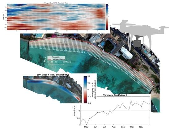
3.1. Surveying
3.2. Three-Dimensional Beach Reconstruction
3.3. Beach Width, Volume, and Surface Area
3.4. Uncertainty
3.5. Empirical Orthogonal Function Analysis
3.6. Shoreline Response to Wave Forcing
4. Results
4.1. Variation in Beach Width
4.2. Changes in Surface Area and Volume
4.3. Empirical Orthogonal Function Analysis
5. Discussion
5.1. Trade-Wind-Driven Transition from Dual Cell to Single Cell Behavior and Generation of Cross-Shore Transport Patterns
5.2. Alternating Rip-Current Formation
5.3. South Swell Energy Flux an Additional Driver of Single Cell Behavior
6. Conclusions
Author Contributions
Funding
Data Availability Statement
Acknowledgments
Conflicts of Interest
References
- Jackson, D.W.T.; Short, A.D. 1—Introduction to Beach Morphodynamics. In Sandy Beach Morphodynamics; Jackson, D.W.T., Short, A.D., Eds.; Elsevier: Amsterdam, The Netherlands, 2020; pp. 1–14. ISBN 978-0-08-102927-5. [Google Scholar]
- Tarui, N.; Peng, M.; Eversole, D. Economic Impact Analysis of the Potential Erosion of Waikīkī Beach. 2018. Available online: https://seagrant.soest.hawaii.edu/wp-content/uploads/2018/08/Economic-Impact-Analysis-Waikiki-Beach-1016-web.pdf (accessed on 1 August 2022).
- Fletcher, C.H.; Romine, B.M.; Genz, A.S.; Barbee, M.M.; Dyer, M.; Anderson, T.R.; Lim, S.C.; Vitousek, S.; Bochicchio, C.; Richmond, B.M. National Assessment of Shoreline Change: Historical Shoreline Change in the Hawaiian Islands; US Department of the Interior, US Geological Survey: Reston, VA, USA, 2012.
- Wiegel, R.L. Waikiki Beach, Oahu, Hawaii: History of Its Transformation from a Natural to an Urban Shore. Shore Beach 2008, 76, 3. [Google Scholar]
- Wang, N.; Gerritsen, F. Nearshore Circulation and Dredged Material Transport at Waikīkī Beach. Coast. Eng. 1995, 24, 315–341. [Google Scholar] [CrossRef]
- Miller, T.L.; Fletcher, C.H. Waikīkī: Historical Analysis of an Engineered Shoreline. J. Coast. Res. 2003, 19, 1026–1043. [Google Scholar]
- Habel, S.; Fletcher, C.H.; Barbee, M.; Anderson, T.R. The Influence of Seasonal Patterns on a Beach Nourishment Project in a Complex Reef Environment. Coast. Eng. 2016, 116, 67–76. [Google Scholar] [CrossRef]
- Dolan, R.; Hayden, B.; Heywood, J. A New Photogrammetric Method for Determining Shoreline Erosion. Coast. Eng. 1978, 2, 21–39. [Google Scholar] [CrossRef]
- Coyne, M.A.; Fletcher, C.H.; Richmond, B.M. Mapping Coastal Erosion Hazard Areas in Hawaii: Observations and Errors. J. Coast. Res. 1999, 171–184. Available online: https://www.jstor.org/stable/25736194 (accessed on 1 August 2022).
- Rooney, J.J.B.; Fletcher, C.H. A High Resolution, Digital, Aerial Photogrammetric Analysis of Historical Shoreline Change and Net Sediment Transport along the Kihei Coast of Maui, Hawaii. In Proceedings of the Thirteenth Annual National Conference on Beach Preservation Technology, Melbourne, FL, USA, 2–4 February 2000. [Google Scholar]
- Genz, A.S.; Fletcher, C.H.; Dunn, R.A.; Frazer, L.N.; Rooney, J.J. The Predictive Accuracy of Shoreline Change Rate Methods and Alongshore Beach Variation on Maui, Hawaii. J. Coast. Res. 2007, 23, 87–105. [Google Scholar] [CrossRef]
- Romine, B.M.; Fletcher, C.H. A Summary of Historical Shoreline Changes on Beaches of Kauai, Oahu, and Maui, Hawaii. J. Coast. Res. 2013, 29, 605–614. [Google Scholar] [CrossRef]
- Rahman, A.A.A.; Awang, N.A.; Maulud, K.N.A.; Hamzah, M.L.; Selamat, S.N.; Mohd, F.A.; Zainal, M.K.; Wahid, M.A.A.; Ariffin, E.H. Multi Method Analysis for Identifying the Shoreline Erosion during Northeast Monsoon Season. J. Sustain. Sci. Manag. 2019, 14, 43–54. [Google Scholar]
- Baig, M.R.I.; Ahmad, I.A.; Shahfahad;Tayyab, M.; Rahman, A. Analysis of Shoreline Changes in Vishakhapatnam Coastal Tract of Andhra Pradesh, India: An Application of Digital Shoreline Analysis System (DSAS). Ann. GIS 2020, 26, 361–376. [Google Scholar] [CrossRef]
- Stockdon, H.F.; Sallenger, A.H.; List, J.H.; Holman, R.A. Estimation of Shoreline Position and Change Using Airborne Topographic Lidar Data. J. Coast. Res. 2002, 18, 502–513. [Google Scholar]
- White, S.A.; Wang, Y. Utilizing DEMs Derived from LiDAR Data to Analyze Morphologic Change in the North Carolina Coastline. Remote Sens. Environ. 2003, 85, 39–47. [Google Scholar] [CrossRef]
- Holman, R.A.; Stanley, J. The History and Technical Capabilities of Argus. Coast. Eng. 2007, 54, 477–491. [Google Scholar] [CrossRef]
- Harley, M.D.; Turner, I.L.; Short, A.D.; Ranasinghe, R. Assessment and Integration of Conventional, RTK-GPS and Image-Derived Beach Survey Methods for Daily to Decadal Coastal Monitoring. Coast. Eng. 2011, 58, 194–205. [Google Scholar] [CrossRef]
- Lomax, A.S.; Corso, W.; Etro, J.F. Employing Unmanned Aerial Vehicles (UAVs) as an Element of the Integrated Ocean Observing System. In Proceedings of the OCEANS 2005 MTS/IEEE, Washington, DC, USA, 17–23 September 2005; pp. 184–190. [Google Scholar] [CrossRef]
- Delacourt, C.; Allemand, P.; Jaud, M.; Grandjean, P.; Deschamps, A.; Ammann, J.; Cuq, V.; Suanez, S. DRELIO: An Unmanned Helicopter for Imaging Coastal Areas. J. Coast. Res. 2009, 6, 1489–1493. [Google Scholar]
- Beretta, F.; Shibata, H.; Cordova, R.; Peroni, R.D.L.; Azambuja, J.; Costa, J.F.C.L. Topographic Modelling Using UAVs Compared with Traditional Survey Methods in Mining. REM-Int. Eng. J. 2018, 71, 463–470. [Google Scholar] [CrossRef]
- Mancini, F.; Dubbini, M.; Gattelli, M.; Stecchi, F.; Fabbri, S.; Gabbianelli, G. Using Unmanned Aerial Vehicles (UAV) for High-Resolution Reconstruction of Topography: The Structure from Motion Approach on Coastal Environments. Remote Sens. 2013, 5, 6880–6898. [Google Scholar] [CrossRef]
- Casella, E.; Rovere, A.; Pedroncini, A.; Stark, C.P.; Casella, M.; Ferrari, M.; Firpo, M. Drones as Tools for Monitoring Beach Topography Changes in the Ligurian Sea (NW Mediterranean). Geo-Mar. Lett. 2016, 36, 151–163. [Google Scholar] [CrossRef]
- Scarelli, F.M.; Sistilli, F.; Fabbri, S.; Cantelli, L.; Barboza, E.G.; Gabbianelli, G. Seasonal Dune and Beach Monitoring Using Photogrammetry from UAV Surveys to Apply in the ICZM on the Ravenna Coast (Emilia-Romagna, Italy). Remote Sens. Appl. Soc. Environ. 2017, 7, 27–39. [Google Scholar] [CrossRef]
- Guisado-Pintado, E.; Jackson, D.W.T.; Rogers, D. 3D Mapping Efficacy of a Drone and Terrestrial Laser Scanner over a Temperate Beach-Dune Zone. Geomorphology 2019, 328, 157–172. [Google Scholar] [CrossRef]
- Casella, E.; Drechsel, J.; Winter, C.; Benninghoff, M.; Rovere, A. Accuracy of Sand Beach Topography Surveying by Drones and Photogrammetry. Geo-Mar. Lett. 2020, 40, 255–268. [Google Scholar] [CrossRef]
- Mikkelsen, A.B.; Anderson, T.R.; Coats, S.; Fletcher, C.H. Complex Drivers of Reef-Fronted Beach Change. Mar. Geol. 2022, 446, 106770. [Google Scholar] [CrossRef]
- Dail, H.J.; Merrifield, M.A.; Bevis, M. Steep Beach Morphology Changes Due to Energetic Wave Forcing. Mar. Geol. 2000, 162, 443–458. [Google Scholar] [CrossRef]
- Turner, I.L.; Harley, M.D.; Drummond, C.D. UAVs for Coastal Surveying. Coast. Eng. 2016, 114, 19–24. [Google Scholar] [CrossRef]
- Hemmelder, S.; Marra, W.; Markies, H.; De Jong, S.M. Monitoring River Morphology & Bank Erosion Using UAV Imagery–A Case Study of the River Buëch, Hautes-Alpes, France. Int. J. Appl. Earth Obs. Geoinf. 2018, 73, 428–437. [Google Scholar]
- Betts, H.D.; Trustrum, N.A.; Rose, R.C.D. Geomorphic Changes in a Complex Gully System Measured from Sequential Digital Elevation Models, and Implications for Management. Earth Surf. Process. Landf. J. Br. Geomorphol. Res. Group 2003, 28, 1043–1058. [Google Scholar] [CrossRef]
- Baldi, P.; Fabris, M.; Marsella, M.; Monticelli, R. Monitoring the Morphological Evolution of the Sciara Del Fuoco during the 2002–2003 Stromboli Eruption Using Multi-Temporal Photogrammetry. ISPRS J. Photogramm. Remote Sens. 2005, 59, 199–211. [Google Scholar] [CrossRef]
- Pesci, A.; Fabris, M.; Conforti, D.; Loddo, F.; Baldi, P.; Anzidei, M. Integration of Ground-Based Laser Scanner and Aerial Digital Photogrammetry for Topographic Modelling of Vesuvio Volcano. J. Volcanol. Geotherm. Res. 2007, 162, 123–138. [Google Scholar] [CrossRef]
- Paul, F.; Haeberli, W. Spatial Variability of Glacier Elevation Changes in the Swiss Alps Obtained from Two Digital Elevation Models. Geophys. Res. Lett. 2008, 35, L21502. [Google Scholar] [CrossRef]
- Wendt, A.; Mayer, C.; Lambrecht, A.; Floricioiu, D. A Glacier Surge of Bivachny Glacier, Pamir Mountains, Observed by a Time Series of High-Resolution Digital Elevation Models and Glacier Velocities. Remote Sens. 2017, 9, 388. [Google Scholar] [CrossRef]
- Berthier, E.; Cabot, V.; Vincent, C.; Six, D. Decadal Region-Wide and Glacier-Wide Mass Balances Derived from Multi-Temporal ASTER Satellite Digital Elevation Models. Validation over the Mont-Blanc Area. Front. Earth Sci. 2016, 4, 63. [Google Scholar] [CrossRef]
- Berthier, E.; Toutin, T. SPOT5-HRS Digital Elevation Models and the Monitoring of Glacier Elevation Changes in North-West Canada and South-East Alaska. Remote Sens. Environ. 2008, 112, 2443–2454. [Google Scholar] [CrossRef]
- Ge, L.; Chang, H.-C.; Rizos, C. Mine Subsidence Monitoring Using Multi-Source Satellite SAR Images. Photogramm. Eng. Remote Sens. 2007, 73, 259–266. [Google Scholar] [CrossRef]
- Carabassa, V.; Montero, P.; Crespo, M.; Padró, J.-C.; Pons, X.; Balagué, J.; Brotons, L.; Alcañiz, J.M. Unmanned Aerial System Protocol for Quarry Restoration and Mineral Extraction Monitoring. J. Environ. Manag. 2020, 270, 110717. [Google Scholar] [CrossRef]
- Padró, J.-C.; Cardozo, J.; Montero, P.; Ruiz-Carulla, R.; Alcañiz, J.M.; Serra, D.; Carabassa, V. Drone-Based Identification of Erosive Processes in Open-Pit Mining Restored Areas. Land 2022, 11, 212. [Google Scholar] [CrossRef]
- Davis, J.M.; Grindrod, P.M.; Boazman, S.J.; Vermeesch, P.; Baird, T. Quantified Aeolian Dune Changes on Mars Derived from Repeat Context Camera Images. Earth Space Sci. 2020, 7, e2019EA000874. [Google Scholar] [CrossRef]
- Qin, R.; Tian, J.; Reinartz, P. 3D Change Detection–Approaches and Applications. ISPRS J. Photogramm. Remote Sens. 2016, 122, 41–56. [Google Scholar] [CrossRef]
- James, L.A.; Hodgson, M.E.; Ghoshal, S.; Latiolais, M.M. Geomorphic Change Detection Using Historic Maps and DEM Differencing: The Temporal Dimension of Geospatial Analysis. Geomorphology 2012, 137, 181–198. [Google Scholar] [CrossRef]
- Sea Engineering, Inc. Final Environmental Assessment Waikiki Beach Maintenance, Prepared for State of Hawaii Department of Land and Natural Resources; Makai Research Pier: Waimanalo, HI, USA, 2010. [Google Scholar]
- State of Hawaii Department of Land and Natural Resources Office of Conservation and Coastal Lands 2021 Waikīkī Beach Maintenance Project. Available online: https://dlnr.hawaii.gov/occl/waikiki/ (accessed on 29 April 2022).
- Clark, J.R.K. Beaches of O‘ahu, Revised Edition; University of Hawai’i Press: Honolulu, HI, USA, 2005. [Google Scholar]
- Gerritsen, F. Beach and Surf Parameters in Hawai’i; University of Hawaii, Sea Grant College Program: Honolulu, HI, USA, 1978; Volume 78. [Google Scholar]
- Homer, P.S. Characteristics of Deep Water Waves in Oʻahu Area for a Typical Year. In Prepared for the Board of Harbor Commissioners, State of Hawaii; Contract No. 5772; Marine Advisors: La Jolla, CA, USA, 1964. [Google Scholar]
- Vitousek, S.; Fletcher, C.H. Maximum Annually Recurring Wave Heights in Hawai’i. Pac. Sci. 2008, 62, 541–553. [Google Scholar] [CrossRef]
- Moberly, R.M.; Chamberlain, T. Hawaiian Beach Systems; Final Report HIG-64-2; Hawaii Institute of Geophysics, University of Hawaii: Honolulu, HI, USA, 1964. [Google Scholar]
- Simpson, R.H. Evolution of the Kona Storm a Subtropical Cyclone. J. Atmospheric Sci. 1952, 9, 24–35. [Google Scholar] [CrossRef]
- Murakami, H.; Wang, B.; Li, T.; Kitoh, A. Projected Increase in Tropical Cyclones near Hawaii. Nat. Clim. Change 2013, 3, 749–754. [Google Scholar] [CrossRef]
- National Oceanic and Atmospheric Administration (NOAA) Tropical Cyclones—Annual 2018|National Centers for Environmental Information (NCEI). Available online: https://www.ncei.noaa.gov/access/monitoring/monthly-report/tropical-cyclones/201813#pac (accessed on 16 May 2019).
- Berg, R.; Houston, S.; Birchard, T. National Hurricane Center/Central Pacific Hurricane Center Tropical Cyclone Report—Hurricane Hector (EP102018). 2019. Available online: https://www.nhc.noaa.gov/data/tcr/EP102018_Hector.pdf (accessed on 1 August 2022).
- Beven, J.L., II; Wroe, D. National Hurricane Center/Central Pacific Hurricane Center Tropical Cyclone Report—Hurricane Lane (EP142018). 2019. Available online: https://www.nhc.noaa.gov/data/tcr/EP142018_Lane.pdf (accessed on 1 August 2022).
- Cangialosi, J.P.; Jelsema, J. National Hurricane Center/Central Pacific Hurricane Center Tropical Cyclone Report—Hurricane Olivia (EP172018). 2019. Available online: https://www.nhc.noaa.gov/data/tcr/EP172018_Olivia.pdf (accessed on 1 August 2022).
- Houston, S.; Birchard, T. Central Pacific Hurricane Center Tropical Cyclone Report—Hurricane Walaka (CP012018). 2020. Available online: https://www.nhc.noaa.gov/data/tcr/CP012018_Walaka.pdf (accessed on 1 August 2022).
- Knapp, K.R.; Kruk, M.C.; Levinson, D.H.; Diamond, H.J.; Neumann, C.J. The International Best Track Archive for Climate Stewardship (IBTrACS): Unifying Tropical Cyclone Best Track Data. Bull. Am. Meteorol. Soc. 2010, 91, 363–376. [Google Scholar] [CrossRef]
- Knapp, K.R.; Diamond, H.J.; Kossin, J.P.; Kruk, M.C.; Schreck, C.J. International Best Track Archive for Climate Stewardship (IBTrACS) Project, Version 4; Eastern Pacific Basin; NOAA National Centers for Environmental Information: Asheville, NC, USA, 2018. Available online: https://www.ncei.noaa.gov/products/international-best-track-archive (accessed on 21 October 2021).
- Norcross, Z.M.; Fletcher, C.H.; Rooney, J.J.B.; Eversole, D.; Miller, T.L. Hawaiian Beaches Dominated by Longshore Transport. Coast. Sediments 2003, 3, 1–15. [Google Scholar]
- Vautherin, J.; Rutishauser, S.; Schneider-Zapp, K.; Choi, H.F.; Chovancova, V.; Glass, A.; Strecha, C.; Sa, D. Photogrammetric Accuracy and Modeling of Rolling Shutter Cameras. ISPRS J. Photogramm. Remote Sens. 2016, 3, 139–146. [Google Scholar] [CrossRef]
- Datums—NOAA Tides & Currents. Available online: https://tidesandcurrents.noaa.gov/datums.html?datum=MSL&units=1&epoch=0&id=1612340&name=Honolulu&state=HI (accessed on 18 April 2022).
- Over, J.-S.R.; Ritchie, A.C.; Kranenburg, C.J.; Brown, J.A.; Buscombe, D.D.; Noble, T.; Sherwood, C.R.; Warrick, J.A.; Wernette, P.A. Processing Coastal Imagery with Agisoft Metashape Professional Edition, Version 1.6—Structure from Motion Workflow Documentation; Open-File Report; U.S. Geological Survey: Reston, VA, USA, 2021. [CrossRef]
- Fletcher, C.H. University of Hawaii Sea Grant College Program (UHSG) Mean Higher High Water (MHHW) Sea Level: Honolulu, Hawaii. Distributed by the Pacific Islands Ocean Observing System (PacIOOS). 2014. Available online: https://www.pacioos.hawaii.edu/metadata/hi_csp_hono_mhhw.html (accessed on 13 November 2018).
- Winant, C.D.; Inman, D.L.; Nordstrom, C.E. Description of Seasonal Beach Changes Using Empirical Eigenfunctions. J. Geophys. Res. 1975, 80, 1979–1986. [Google Scholar] [CrossRef]
- Aubrey, D.G. Seasonal Patterns of Onshore/Offshore Sediment Movement. J. Geophys. Res. Ocean. 1979, 84, 6347–6354. [Google Scholar] [CrossRef]
- Dick, J.E.; Dalrymple, R.A. Coastal Changes at Bethany Beach, Delaware. Coast. Eng. Proc. 1984, 1, 112. [Google Scholar] [CrossRef]
- Losada, M.A.; Medina, R.; Vidal, C.; Roldán, A. Historical Evolution and Morphological Analysis of “El Puntal” Spit, Santander (Spain). J. Coast. Res. 1991, 7, 711–722. [Google Scholar]
- Anderson, T.R.; Neil Frazer, L.; Fletcher, C.H. Transient and Persistent Shoreline Change from a Storm. Geophys. Res. Lett. 2010, 37. [Google Scholar] [CrossRef]
- Cheung, K.F. Simulating WAves Nearshore (SWAN) Regional Wave Model: Oahu. April–December 2018 Distributed Pacific Islands Ocean Observing System (PacIOOS). Available online: https://www.pacioos.hawaii.edu/metadata/swan_oahu.html (accessed on 18 February 2019).
- McManus, M.A.; Merrifield, M.A. Pacific Islands Ocean Observing System (PacIOOS) PacIOOS Wave Buoy 098: Mokapu Point, Oahu, Hawaii. January 2018–February 2020. Wave Energy Flux (South Swell). Distributed by the Coastal Data Information Program (CDIP). 2000. Available online: http://www.pacioos.hawaii.edu/metadata/cdip098.html?format=fgdc (accessed on 23 March 2020).
- McManus, M.A.; Merrifield, M.A. Pacific Islands Ocean Observing System (PacIOOS) PacIOOS Wave Buoy 233: Pearl Harbor Entrance, Oahu, Hawaii January 2018–February 2020. Wave Energy Flux (Trade-Wind Waves). Distributed by the Coastal Data Information Program (CDIP). 2017. Available online: https://www.pacioos.hawaii.edu/metadata/cdip233.html (accessed on 23 March 2020).
- Dean, R.G.; Dalrymple, R.A. Coastal Processes with Engineering Applications; Cambridge University Press: Cambridge, UK, 2004. [Google Scholar]


| Tropical Cyclone | Dates of Influence | Peak Intensity |
|---|---|---|
| Hurricane Hector | 9 August 2018–15 August 2018 | Category 4, 250 km/h |
| Hurricane Lane | 20 August 2018–27 August 2018 | Category 5, 259 km/h |
| Tropical Storm Olivia | 10 September 2018–14 September 2018 | Category 4, 213 km/h |
| Hurricane Walaka | 2 October 2018–6 October 2018 | Category 5, 259 km/h |
Publisher’s Note: MDPI stays neutral with regard to jurisdictional claims in published maps and institutional affiliations. |
© 2022 by the authors. Licensee MDPI, Basel, Switzerland. This article is an open access article distributed under the terms and conditions of the Creative Commons Attribution (CC BY) license (https://creativecommons.org/licenses/by/4.0/).
Share and Cite
McDonald, K.K.; Fletcher, C.H.; Anderson, T.R.; Habel, S. Weekly Small Uncrewed Aerial System Surveys, Structure from Motion, and Empirical Orthogonal Function Analyses Reveal Unique Modes of Sediment Exchange Generated by Seasonal and Episodic Phenomena: Waikīkī, Hawaiʻi. Remote Sens. 2022, 14, 5108. https://doi.org/10.3390/rs14205108
McDonald KK, Fletcher CH, Anderson TR, Habel S. Weekly Small Uncrewed Aerial System Surveys, Structure from Motion, and Empirical Orthogonal Function Analyses Reveal Unique Modes of Sediment Exchange Generated by Seasonal and Episodic Phenomena: Waikīkī, Hawaiʻi. Remote Sensing. 2022; 14(20):5108. https://doi.org/10.3390/rs14205108
Chicago/Turabian StyleMcDonald, Kristian K., Charles H. Fletcher, Tiffany R. Anderson, and Shellie Habel. 2022. "Weekly Small Uncrewed Aerial System Surveys, Structure from Motion, and Empirical Orthogonal Function Analyses Reveal Unique Modes of Sediment Exchange Generated by Seasonal and Episodic Phenomena: Waikīkī, Hawaiʻi" Remote Sensing 14, no. 20: 5108. https://doi.org/10.3390/rs14205108
APA StyleMcDonald, K. K., Fletcher, C. H., Anderson, T. R., & Habel, S. (2022). Weekly Small Uncrewed Aerial System Surveys, Structure from Motion, and Empirical Orthogonal Function Analyses Reveal Unique Modes of Sediment Exchange Generated by Seasonal and Episodic Phenomena: Waikīkī, Hawaiʻi. Remote Sensing, 14(20), 5108. https://doi.org/10.3390/rs14205108