Remote Sensing of Chlorophyll-a in Xinkai Lake Using Machine Learning and GF-6 WFV Images

Abstract

Lake ecosystem eutrophication is a crucial water quality issue that can be efficiently monitored with remote sensing. GF-6 WFV with a high spatial and temporal resolution provides a comprehensive record of the dynamic changes in water quality parameters in a lake. In this study, based on GF-6 WFV images and the field sampling data of Xingkai Lake from 2020 to 2021, the accuracy of three machine learning models (RF: random forest; SVR: support vector regression; and BPNN: back propagation neural network) was compared by considering 11 combinations of surface reflectance in different wavebands as input variables for machine learning. We mapped the spatiotemporal variations of Chl-a concentrations in Xingkai Lake from 20192021 and integrated machine learning algorithms to demonstrate that RF obtained a better degree of derived-fitting (Calibration: N = 82, RMSE = 0.82 μg/L, MAE = 0.57 μg/L, slope = 0.94, and R² = 0.98; Validation: N = 40, RMSE = 2.12 μg/L, MAE = 1.58 μg/L, slope = 0.91, R² = 0.89, and RPD = 2.98). The interannual variation from 2019 to 2021 showed that the Chl-a concentration in Xingkai Lake was low from June to July, while maximum values were observed from October to November, thus showing significant seasonal differences. Spatial distribution showed that Chl-a concentrations were higher in Xiao Xingkai Lake than in Da Xingkai Lake. Nutrient inputs (N, P) and other environmental factors such as high temperature could have an impact on the spatial and temporal distribution characteristics of Chl-a, therefore, combining GF-6 WFV satellite images with RF could realize large-scale monitoring and be more effective. Our results showed that remote-sensing-based machine learning algorithms provided an effective method to monitor lake eutrophication as well as technical support and methodological reference for inland lake water quality parameter inversion.

1. Introduction

Eutrophication is a concerning issue in most lakes [1], considering the increase in Chlorophyll-a (Chl-a) concentration and the frequency of algal blooms [2,3]. Global warming, in particular, affects the physicochemical properties of lakes [4]; for example, an increased lake temperature could reduce nutrient flows from deep waters to the surface, thereby decreasing the primary productivity of lake ecosystems. Likewise, human activities have contributed to the deterioration of water quality through agricultural activities, aquaculture [5], and industrial and domestic wastewater [6], owing to the food demands of the increasing population [7]. Chl-a, a photosynthetic pigment found in algae species [8], has been considered the largest weighted factor to calculate the Carlson trophic state indices [9]. Assessments of the timing and extent of algal biomass and eutrophication states in aquatic ecosystems may frequently be performed using extensive long-term Chl-a concentration measurements [10]. These eutrophication insights can help us understand primary production, biogeochemical cycling, and overall inland water quality, which can result in environmental changes and useful mitigation tactics [11,12].

Khanka Lake (Xingkai Lake in Chinese), located on the Sanjiang Plain, provides tourism, irrigation, aquaculture, and drinking water for the surrounding residents. With increasing population and rapid economic growth, there have been serious environmental issues in Xingkai Lake, including 11 algal bloom events in Da Xingkai Lake and 5 algal bloom events in Xiao Xingkai Lake [13]. These blooms greatly reduce the ability of the lake ecosystem to recover and increase the environmental pressures on the aquatic ecosystems [14]. Eutrophication of Xingkai Lake has been recognized as a severe issue [15]; therefore, it is necessary to investigate its spatiotemporal variations to suggest the requirements for eutrophication research.

Xingkai Lake is a Sino-Russian international border lake, and the management and protection of the lake can help to maintain the friendship between the two countries [16]. For many decades, Chl-a measurements in lakes have been a considerable issue since traditional sampling is a time-consuming and labor-intensive process and in situ data cannot represent the entire lake. Satellite remote sensing is a helpful instrument for monitoring inland waters with several benefits [17], including its low cost and continuous monitoring. Remote sensing can make up for the deficiencies of traditional sampling. Remote sensing technology helps us comprehensively integrate water safety management at national and watershed scales and provides information support for lake water quality evaluation.

There are no satellite sensors specifically designed for inland water [18]. Monitoring Chl-a dynamics still uses ocean color satellite sensors, including the Moderate Resolution Imaging Spectroradiometer (MODIS) [19], the Ocean and Land Color Instrument (OLCI) [12,20], and the Medium Resolution Imaging Spectrometer (MERIS) [21]. Additionally, some land observation satellites have been applied, for example, Landsat and Sentinel series satellites and Satellite pour l’Observation de la Terre (SPOT) [22,23]. Satellite sensor data with high spatiotemporal resolutions are required for timely monitoring due to the rapidly changing water quality conditions and complex optical composition of inland lakes. The GF-6 satellite can satisfy these requirements simultaneously. The GF-6 satellite was launched and orbited on June 2, 2018, and has provided 16-m spatial resolution data from wide-format cameras (WFV) and a 4-d revisit time [24]. The single-camera regime allows for ultra-large-format imaging for visual remote sensing interpretation. The satellite radiation performance is good, and the camera system exhibits excellent performance with a high signal-to-noise ratio, wide dynamic range, and high internal geometric accuracy [25]. Natural lakes all experience the transition from an initial state of poor to eutrophic, and the dynamic changes of water quality parameters of lakes under the nutrient state were recorded by the multi-spectral medium-resolution wide-format sensor of the GF-6. Remote sensing data and measured water quality indicators could be used to establish eutrophication evaluation methods for lakes, which could concretize this evolutionary process in lakes. The more clearly digitized results could provide a scientific basis for water environment management and help to govern decision making. Moreover, the ability to quantify water quality using the GF-6 satellite is still insufficient; it was necessary to complement the datasets and validation gap.

In recent decades, remote sensing technology has provided access to substantial information for lake monitoring [18]. Previous studies have developed various Chl-a algorithms, including empirical, bio-optical, semi-empirical/semi-analytical, and machine learning models. Empirical algorithms are relatively simple and easy to implement, as they are based on statistical analysis and Chl-a spectral features. Some simple band algorithms, such as the blue-green band ratio [26], two-band [27], three-band [11], and four-band algorithms [28], are also available. The analytical algorithm, which is based on the physical basis of radiative transfer, mainly uses the relationship between the water composition and inherent optical properties and apparent and intrinsic optics to simulate the water environment and invert water quality parameters [22,29]; however, semi-analytical algorithms, such as Chl-a specific absorption and particulate matter backscattering coefficients [30], often need to be parameterized in a particular lake. Machine learning models have been the most popular approach for data estimation in recent years and have been successfully developed to model complex relationships, such as nonlinearities [31]. Random forest (RF) algorithms, support vector machine regression (SVR) algorithms, and back propagation neural networks (BPNN) are widely used machine learning models that can solve nonlinear relationships. RF has good generalization capabilities and it uses regression tree ensembles for data estimation; therefore, it is often used to predict the Chl-a concentration [32,33]. In this study, we developed three machine learning algorithms to quantify Chl-a concentration using GF-6 WFV satellite images and evaluated the model’s performances, aiming to find a reliable model for mapping the spatial and temporal variation of Chl-a concentration.

2. Materials and Methods

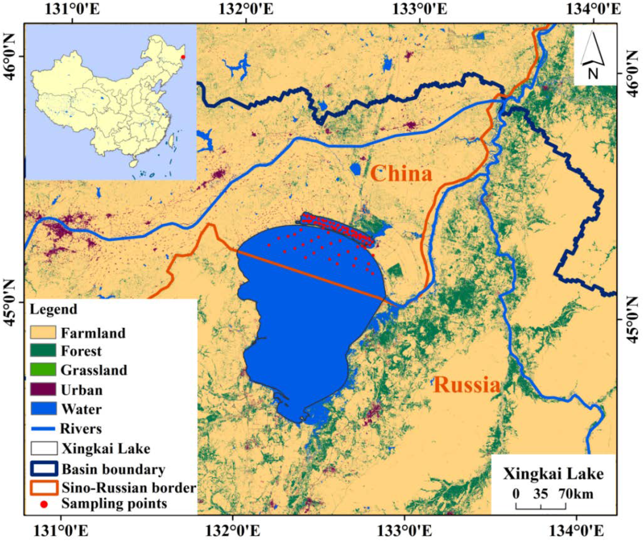
2.1. Study Area

Xingkai Lake (44°27′N45°23′N, 131°58′E132°52′E) is an international boundary region between Russia and China (Figure 1). There is a natural wall dividing the lake into the Da Xingkai and Xiao Xingkai lakes, however, a third of the surface area of Da Xingkai and all of Xiao Xingkai belong to China (a total of 1080 km²), while the rest belongs to Russia (3080 km²) [34]. The lake capacity of Da Xingkai is approximately 17.5 billion m³, while that of Xiao Xingkai is approximately 3.3 billion m³ [35,36]. In total, there are 20 main inflowing rivers and three outflowing rivers, with a water residence time of 8.8 years [37]. The ice-free period of Lake Xingkai lasts from April to October, that is, approximately 210 days.

2.2. Data Acquisition and Processing

2.2.1. Field Sampling

Two years of in situ lake samples were collected from October 2020 to 2021, capturing 122 samples (Figure 1). These samples were collected during days with clear, cloudless, or less cloudy weather conditions absent of wind or breeze. Using 2 L High Density Polyethylene (HDPE) bottles, lake water samples were taken at each location at depths of approximately 0.5 m. The bulk bottles were then transferred to the laboratory for analysis within 24 h, where they were immediately stored at 4 °C in a portable refrigerator. Prior to sampling, each bottle was acid-cleaned and rinsed with distilled water. The Secchi disk depth (SDD, cm) was measured using a black-and-white Secchi disk.

2.2.2. Experimental Analysis

In the laboratory, a portion of each water sample was filtered through a 0.45 μm mixed fiber millimeter filter (Bandao Industrial Co., Chengdu, China). Chl-a was extracted using a 90% buffered acetone solution immersed in dark conditions for 24 h. The concentrations were calculated using coefficients measured at 750, 663, 645, and 630 nm with a UV-2600 PC (UV-2600 PC, Shimadzu) spectrophotometer according to the SCOR-UNESCO formula [38,39]. The concentrations (mg/L) of total nitrogen (TN) and total phosphorus (TP) were obtained using a continuous flow analyzer (SKALAR, San Plus System, Delft, The Netherlands). The turbidity of each water sample was spectrophotometrically measured in the laboratory [40].

The water samples were again filtered through a 0.7-µm glass fiber membrane (Whatman, GF/F1825-047) to retain particulate matter, and separately through a 0.22-µm polycarbonate membrane (Whatman, 110606). According to the quantitative membrane filter technique [41], the optical density (OD) of the colored dissolved organic matter (CDOM) was measured using a UV-2600PC spectrophotometer at 200 to 800 nm. The absorption coefficient of the CDOM at 440 nm was selected to represent the CDOM level. A UV-2600PC spectrophotometer was used to measure the absorption coefficients of total particulate matter, algae, and non-algae particulate matter in the water samples.

2.2.3. Satellite Data Acquisition and Pre-Processing

GF-6 WFV images were obtained from the Land Observation Satellite Service (http://36.112.130.153:7777/#/home (accessed on 27 August 2022)). The spatial resolution of the images was 16 m, and the revisit period of the GF-6 satellite was 4 days. There were eight wavelength bands (Table S1). Altogether, 17 scenes of cloud-free GF-6 WFV pictures encompassing the lake were retrieved with a temporal range of ±3 d from in situ measurements. The original images were pre-processed by radiometric calibration and FLAASH atmospheric correction to convert the brightness information into reflectance. A 3 × 3 window containing pixels with an average reflectance that matched the location of the sampling point was extracted. The normalized difference water index (NDWI) was used to obtain the boundary of the Xingkai Lake water body (the formula is shown in the Supporting Materials) [42]. All processes were performed using ENVI 5.3 software (Figure 2).

2.3. Machine Learning Models Based on Chl-a Algorithms

2.3.1. Random Forest

RF is an ensemble machine learning method to create nonlinear functions based on the mean response of a group of smaller decision tree models [43,44]. The random forest theory entails creating a forest with multiple unconnected decision trees. The purpose of this forest is to perform a classification operation that involves entering each sample data into each decision tree separately to identify which class the data should belong to. Ultimately, whichever class of sample data has the most data is predicted to be that class. In this study, the RF was run using the python 3.8 platform, and the detailed configurations included 500 regression trees (ntree) where the depth of each tree was 15, the minimum number of samples of leaf nodes was 1, and the minimum number of samples of node splitting was 2.

2.3.2. Support Vector Regression

Support vector regression (SVR) was used to perform regression analysis by introducing an insensitive loss function to project the data into a higher-dimensional feature space through a nonlinear mapping as Statistical Learning Theory (SLT). Based on the strict mathematical theory, the SVR aims to improve the model’s reliability, particularly for small sample sizes [45]. SVR converts the research problem into a high-dimensional feature space, where it creates a nonlinear regression by constructing a linear regression connection in the high-dimensional space. The format of SVR can be expressed as follows:

$$f\left(x\right)=w\times \phi \left(x\right)+b$$

(1)

where w is the normal vector and b is the offset. In the nonlinear case, the sample x can be mapped to the high-dimensional feature space K by nonlinear mapping $\phi \left(x\right)$ in K, in which the regression function is derived. The linear fit of the nonlinear transformation is achieved by using an appropriate kernel function K(x_i x) in the regression function instead of the vector inner product $\phi \left(xi\right)$·$\phi \left(x\right)$ in the high-dimensional space. The corresponding regression functions and normal vectors are:

$$f(x)={\displaystyle {\sum }_{i=1}^l(}\alpha \iota -\alpha \iota *)K(x\iota \cdot x)+b$$

(2)

$$w={\displaystyle {\sum }_{i=1}^l(}\alpha \iota -\alpha \iota *\left)K\right(x\iota \cdot x)$$

(3)

where a_i and a* are the auxiliary variables. SVR was conducted using the python 3.8 platform. The kernel function, kernel default rbf, is an exponential prediction with penalty parameters C = np.power (0.5,2), gamma = np.power (2,0.0).

2.3.3. Back Propagation Neural Network

The back propagation neural network (BPNN) model is a widely used machine learning method for quantifying water quality parameters and generating water color products [46]. The BPNN could constitute a nonlinear mapping from input to output by simulating the structure of connections between biological neurons. By adjusting the connection weights between neurons, the error is propagated and repaired. A 3-layer BPNN model containing an input layer, implicit layer, and output layer was constructed in this study using the python 3.8 platform. The input layer was the band combinations of the surface reflectance extracted from GF-6 WFV images, the output layer was the Chl-a concentration, and the number of neurons in the hidden layer was set to 140 by experimental comparison and analysis.

2.3.4. Input Variables for Machine Learning Models

In this study, the surface reflectance of GF-6 WFV images was used as an input variable, and the predicted Chl-a concentration values were used as output values.

When all datasets were pooled together, 2/3 (N = 82) of the 122 samples were randomly selected as the calibration dataset, while the remaining 1/3 (N = 40) samples were the validation dataset. The random grouping of datasets was implemented based on Matlab2015b software. Using the Spearman correlation analysis (two-tailed test), the Chl-a concentration showed a good correlation (r > 0.6) with the blue (B1), green (B2), coastal blue (B7), and yellow (B8) bands of the GF-6 satellite (Table S1). These may be employed as sensitive bands related to Chl-a with correlation coefficients of −0.72 **, −0.66 **, −0.87 **, and −0.64 **, respectively. Finally, the following band combinations were developed as sensitive input variables bands responding to Chl-a levels: B1 + B2, B1 + B7, B1 + B8, B2 + B7, B2 + B8, B7 + B8, B1 + B2 + B7, B1 + B2 + B8, B2 + B7 + B8, B1 + B7 + B8, and B1 + B2 + B7 + B8 (“B” represented the surface reflectance of GF-6 WFV images) (Tables S2 and S3).

2.4. Chl-a Estimation in Xingkai Lake with GF-6

With our developed machine learning-based Chl-a model, the images acquired from June to November 2019 to 2021 was used to generate spatiotemporal maps of Chl-a levels. The details of the pre-processing of the radiometric calibration and FLAASH processor can be found in Section 2.2.3, Supporting Materials (method), and Figure 2. Furthermore, image data acquired in the summer/autumn were used because there was less cloud contamination [47]. Altogether, 17 scenes from the GF-6 images were used to map Chl-a. The inland water body mask described in Section 2.2.3 was used to clip the Chl-a map results.

2.5. Statistical Analysis and Accuracy Evaluation

Statistical analysis was performed using IBM SPSS Statistics 26 software, including the Spearman correlation, Pearson correlation (r means correlation coefficient), analysis of variance (ANOVA), and regression analysis. To evaluate the performance of the models, we calculated the coefficient of determination (R²), root mean square error (RMSE), mean absolute error (MAE), and relative predictive deviation (RPD) for linear fitting between the measured and estimated values [48]. Details of the statistical analysis and accuracy evaluations can be found in the Supporting Materials.

3. Results and Discussion

3.1. Water Qualities Characteristics and Environmental Effects

3.1.1. Water Qualities and Optical Properties

According to

Table 1. The statistical description of water quality parameters in Xiao Xingkai (XXK) and Da Xingkai Lake (DXK).

	Date	Parameter	N	Min.	Max.	Mean	SD.
XXK	2020.10	Chl-a (µg/L)	10	1.46	4.51	2.56	0.98
		TSM (mg/L)	10	57.06	199.17	144.31	41.69
		SDD (cm)	10	-	-	-	-
		Turbidity (NTU)	10	69.39	297.51	200.48	62.85
		TN (mg/L)	10	0.85	1.37	1.11	0.18
		TP (mg/L)	10	0.12	0.20	0.17	0.02
	2021.08	Chl-a (µg/L)	6	0.81	3.55	2.65	1.02
		TSM (mg/L)	6	22.00	43.85	29.55	7.92
		SDD (cm)	6	24.00	35.00	30.40	4.41
		Turbidity (NTU)	6	29.70	70.11	50.57	13.66
		TN (mg/L)	6	1.18	9.66	4.52	3.17
		TP (mg/L)	6	0.06	0.37	0.19	0.13
	2021.09	Chl-a (µg/L)	19	3.96	7.99	5.93	1.19
		TSM (mg/L)	19	28.00	66.00	44.41	9.54
		SDD (cm)	19	16.00	27.00	21.00	3.75
		Turbidity (NTU)	19	43.23	74.76	57.23	8.45
		TN (mg/L)	19	0.33	0.49	0.40	0.04
		TP (mg/L)	19	0.09	0.27	0.16	0.05
	2021.10	Chl-a (µg/L)	45	9.78	23.95	15.29	3.06
		TSM (mg/L)	45	30.00	297.50	111.63	52.05
		SDD (cm)	45	13.00	31.00	19.89	3.77
		Turbidity (NTU)	45	46.63	439.60	163.63	78.40
		TN (mg/L)	45	0.36	0.58	0.44	0.05
		TP (mg/L)	45	0.05	0.34	0.16	0.08
DXK	2020.10	Chl-a (µg/L)	10	2.98	7.92	4.85	1.64
		TSM (mg/L)	10	85.00	216.00	119.42	40.30
		SDD (cm)	10	10.00	20.00	14.00	3.46
		Turbidity (NTU)	10	85.90	226.13	126.21	41.60
		TN (mg/L)	10	0.43	0.77	0.50	0.16
		TP (mg/L)	10	0.12	0.20	0.17	0.02
	2021.06	Chl-a (µg/L)	31	0.14	4.05	1.46	1.03
		TSM (mg/L)	31	56.67	106.43	81.05	13.17
		SDD (cm)	31	14	21	17.16	1.93
		Turbidity (NTU)	31	57.39	112.16	85.08	15.76
		TN (mg/L)	31	0.57	0.72	0.66	0.05
		TP (mg/L)	31	0.08	0.29	0.21	0.04

, we found that maximum, minimum, and average values of the Chl-a concentration in Xiao Xingkai Lake showed an increasing tendency in the order August (3.977.99 μg/L, 2.65 ± 1.02 μg/L) > September (3.97–7.99 μg/L, 5.93 ± 1.19 μg/L) > October (9.78–23.95 μg/L, 16.29 ± 3.06 μg/L). For Da Xingkai Lake, October (2.98–7.92 μg/L, 4.85 ± 1.64 μg/L) had higher Chl-a concentrations than June (0.14–4.05 μg/L, 1.46 ± 1.03 μg/L). Significant temporal variations were observed (Xiao Xingkai, ANOVA, F = 23.911, p < 0.001; Da Xingkai, ANOVA, F = 62.899, p < 0.001) which was largely consistent with the dynamics of Chl-a concentrations in most northeast cold lakes [49]. Of which, the Chl-a levels ranged from 0.11 to 20.41 μg/L in seven investigated northeast lakes, and the highest Chl-a was found in autumn (September and October). This may be due to the legacy effect of nutrients from watersheds [49], where accumulation in cropland continues to mobilize for a long time after soil leaching and runoff inputs. For lakes, a brief pre-winter bloom of phytoplankton and an increased Chl-a concentration in the water body were observed [50]. Additionally, other water qualities, such as TSM, turbidity, and SDD, also showed a similar temporal following the order October > September > August.

3.1.2. Chl-a versus Water Biogeochemistry

Many environmental factors could affect the levels of Chl-a, such as nutrient inputs of runoff via soil leaching, low water self-clarification ability introduced by decreasing water elevation, and sediment resuspended by wind [51]. The correlation between Chl-a and the other water quality parameters was also examined (Figure 3). For Da Xingkai, there were moderate negative correlations among Chl-a, TN (r = −0.51, 2-tails, p < 0.01), and TP (r = −0.36, 2-tails, p < 0.05). Likewise, a correlation between Chl-a and TN (r = −0.39, 2-tails, p < 0.01) was found in Xiao Xingkai, consistent with the conclusion of Kang et al. [15] regarding the relationship between water quality parameters in Xingkai Lake. Other findings also showed that the correlation relationships (between Chl-a and TN or Chl-a and TP) were related to TN/TP values. When the values exceeded a certain threshold, the Chl-a concentration was negatively correlated with the TN and TP [52].

Moreover, high temperatures and other environmental factors could cause phytoplankton to sink, resulting in small chlorophyll measurements. Numerous paddy fields are distributed around Xingkai Lake, resulting in the lake becoming more affected by agricultural surface source pollution. When farming started, a large amount of organic fertilizer entered Xingkai Lake or its in-lake rivers with increased nutrients. When the external nutrient load was reduced, nutrients in the lake sediment could be gradually released to supplement the nutrients in the water. The release of endogenous nutrients increased the total nitrogen and phosphorus in the lake and led to a decrease in chlorophyll content and an increase in total nitrogen and phosphorus content.

3.2. Remote Sensing Reflectance Characteristics

The surface reflectance on the GF-6 WFV image was converted to remote sensing reflectance (Rrs) by band math in ENVI (see supporting material for the equation). The reflectance spectra of the sampling sites and their corresponding CV are shown (Figure 4), and Rrs (λ) presents great variability owing to the highly variable water quality compositions. Owing to noise beyond 800 nm, the spectral range of 400 to 800 nm was chosen to investigate the spectral characteristics. This is due to the strong absorption of Chl-a, CDOM, and TSM in the short-wavelength domain from 400 to 500 nm. The peak of the remote sensing reflectance is shown in green, owing to the scattering of suspended particulate matter, especially in turbid waters. At approximately 660 nm, there was a slight turn, indicating that phytoplankton absorption was covered by other optically active substances. All reflectances in the 700 to 790 nm spectral band were largely regulated by particle scattering and pure water absorption.

3.3. Chlorophyll-a Model Calibration and Validation

Band combinations correlating to Chl-a concentrations using multi-linear regression were developed and used as input variables for RF, SVR, and BPNN (Tables S2 and S3). The statistical metrics computed using the calibration datasets (N = 122) indicate that three machine learning algorithms (RF, R² = 0.98, RPD = 2.98, RMSE = 2.98 μg/L, MAE = 0.57 μg/L; SVR, R² = 0.86, RPD = 2.73, RMSE = 2.41 μg/L, MAE = 1.88 μg/L; and BPNN, R² = 0.88, RPD = 2.43, RMSE = 0.85 μg/L, MAE = 2.46 μg/L) showed good performances (Figure 5). Additionally, the results using the validation datasets showed that three machine learning algorithms (RF, R² = 0.88, RPD = 2.98, RMSE = 0.82 μg/L, MAE = 0.57 μg/L; SVR, R² = 0.80, RPD = 2.73, RMSE = 2.78 μg/L, MAE = 2.78 μg/L; and BPNN, R² = 0.88, RPD = 2.43, RMSE = 2.60 μg/L, MAE = 1.80 μg/L) also showed good performances (Figure 5). The errors in the estimated and measured values for the three models are shown in Figure S3. Compared with BPNN and SVR, the RF model had a higher fitting accuracy; not only did it have the lowest error, but its linear model also had the slope closest to 1. The RPD value of the RF model was nearly 3, which indicated excellent model prediction performance. Although the RPD values of both BPNN and SVR showed the usability of the model, the RF model was more stable. Even for the dataset containing high Chl-a values, the dispersion of the data prediction results from the RF was minimal, and the model performed satisfactorily. Hence, we used the RF Chl-a model to quantify and map Chl-a concentration.

Generally, because trees are diverse and unpruned, RF is often more accurate than single-decision trees. Each RF tree is created using a random sample, and a random set of features is considered for splitting at each node. The trees become diverse because of these procedures. It can effectively handle nonlinear and non-Gaussian data without assuming a probability distribution for the data or experiencing overfitting issues as the number of trees rises [44]. Li et al. [32] used an RF model to invert the Chl-a concentration in Poyang Lake from 2008 to 2014. By contrast, SVR is sensitive to missing data, and the choice of kernel functions can manage high-dimensional features [7]. For BPNN, networks with several implicit layers can be found, and there is currently no rapid and accurate approach to determine the parameters (including hidden layer sizes and random states); hence, the empirical estimation can only be used to estimate a wide range which has an impact on the reasonable settings for these parameters [53]. As a result, the BPNN relied heavily on the sizes and ranges of the training samples. The BP algorithm uses a gradient steepest descent method that may converge to a local minimum, which has drawbacks in terms of balanced predictive power [54]. Therefore, in this study, the RF Chl-a model outperformed other machine-learning algorithms.

3.4. Chlorophyll-a Distributions of Xingkai Lake

3.4.1. Temporal Distribution Characteristics

Using the RF Chl-a model, the monthly mean, maximum, and minimum values of the Chl-a concentration in the non-ice period (June to November,

Table 2. Mean, maximum, minimum, and standard deviation of Chl-a concentration (unit: µg/L) in GF-6 WFV images of Xiao Xingkai Lake.

Date	Mean ± SD	MinMax	Date	Mean ± SD	MinMax	Date	Mean ± SD	MinMax
201906	9.30 ± 1.60	2.4616.02	202006	4.44 ± 1.84	1.9719.45	202106	1.41 ± 0.53	0.507.74
201907	4.06 ± 0.99	2.5116.23	202007	2.33 ± 1.32	0.607.94	202107	2.60 ± 0.21	0.507.84
			202008	4.78 ± 3.38	2.1220.77	202108	2.08 ± 0.17	1.377.69
201909	14.49 ± 2.83	2.5420.55	202009	2.66 ± 0.26	0.667.76	202109	6.62 ± 2.41	1.2220.32
201910	10.73 ± 0.46	2.6219.14	202010	3.26 ± 1.09	1.4519.67	202110	14.82 ± 1.64	2.0121.01
201911	15.10 ± 2.37	2.6220.55	202011	2.08 ± 0.50	0.4418.58	202111	7.87 ± 3.41	2.0519.79

and

Table 3. Mean, maximum, minimum, and standard deviation of Chl-a concentration (unit: µg/L) in GF-6 WFV images of Da Xingkai Lake.

Date	Mean ± SD	MinMax	Date	Mean ± SD	MinMax	Date	Mean ± SD	MinMax
201906	7.34 ± 2.83	2.4817.72	202006	2.63 ± 0.68	1.2319.33	202106	1.30 ± 0.53	0.367.84
201907	5.34 ± 2.09	2.0618.60	202007	1.77 ± 0.84	0.3618.48	202107	2.57 ± 0.40	0.4719.21
			202008	3.53 ± 2.63	1.5420.54	202108	2.25 ± 0.12	0.817.68
201909	10.72 ± 1.67	2.6220.46	202009	2.53 ± 0.60	0.4819.64	202109	5.04 ± 1.66	0.4920.43
201910	11.47 ± 1.54	2.5620.08	202010	3.85 ± 1.50	1.6720.50	202110	11.50 ± 2.25	1.8920.40
201911	11.39 ± 1.63	2.6220.46	202011	2.36 ± 0.85	0.4220.36	202111	3.03 ± 0.80	1.4019.79

) from 2019 to 2021 were quantified using the average values of the image pixels (Figure 6). The monthly Chl-a concentration ranged from 0 to 21 μg/L, with average Chl-a values ranging from 1.31 to 15.30 μg/L. There were significant annual variations in the Chl-a levels that followed the order 2019 > 2021 > 2020.

The Chl-a levels in the Da Xingkai and Xiao Xingkai Lakes increased significantly from October 2019 to 2021, which was consistent with our seasonal dynamics of in situ Chl-a concentrations. From June to September 2021, the Chl-a concentration in Da Xingkai Lake was maintained at a low level, not exceeding 15 g/L. In October, there was an abrupt increase, with an average value of 11.50 g/L and a high value of 20.40 g/L. As mentioned previously, the legacy effect of lake nutrients remained a major cause of elevated Chl-a concentration. However, in Xiao Xingkai Lake, there was a noticeable decline in October 2019. The nitrogen cycle of the lake was disturbed during tourism or fishing activities, suggesting that it could have been caused by human influence. Another potential explanation was that the decrease in temperature and the corresponding decline in microbial activity caused the concentration of Chl-a to increase.

From June to November 2020, there were no apparent variations in the Chl-a concentration in Da Xingkai Lake; however, the value was lower than that of Xiao Xingkai Lake. Additionally, the average Chl-a concentration from June to July decreased, as shown by Xiao and Da Xingkai in 2019 and 2020. The Chl-a signal and color were covered by suspended sediment in the water introduced by hydrological processes.

3.4.2. Spatial Distribution Characteristics

Generally, the Chl-a concentrations were much higher in the southern part of Da Xingkai Lake (Russia) than in the northern (China). The southern portion of Xingkai Lake is shallow and displays some characteristics of wetlands so some vegetation signals might cause the inversion results of Chl-a to be excessively high in this area. It was also considered that the cultural differences between the two countries led to different disturbances by human activities in the northern and southern regions of Xingkai Lake, resulting in the great diversity in the spatial distribution of Chl-a concentration. Simultaneously, the Chl-a levels in Xiao Xingkai Lake were more variable than those in Da Xingkai Lake (Figure 7). The deeper depth and larger area of the lake weakened the influence of environmental factors on the variations of water quality parameters. Both the depth and area of Da Xingkai Lake are greater than that of Xiao Xingkai Lake, so it is more inclusive and less susceptible to disturbance.

Spatial distributions of Chl-a changes can be site-specific; Chl-a levels in the southwest part of the Da Xingkai Lake were low in June 2020, within the range of 0–2.2 μg/L; Chl-a concentration in the middle of Da Xingkai Lake did not significantly change in the months of June, July, and August; Chl-a concentration increased noticeably in the east, south, and west coastline waters of the Xiao Xingkai Lake; and Chl-a levels in Da Xingkai Lake declined from September to November 2020, falling to below 2.0 g/L, but they remained higher than in July; however, in November, the concentration of Chl-a in the southern Da Xingkai Lake rose once again, reaching a level of approximately 4.0 g/L. With weak spatial heterogeneity, Xiao Xingkai Lake displayed the same trend as Da Xingkai Lake in 2020, and the distribution of Chl-a concentration was shown to be uniform. The year 2020 was the year of the coronavirus disease 2019 (COVID-19) outbreak. Because of the epidemic, human activities such as tourism and agriculture were reduced, which might have made the hydrological status of the lake stable.

In June 2021, there was a large discrepancy in the Chl-a concentration of the lake between the east and west. Overall, the lake had a low Chl-a content, with no obvious change from July to August 2021. The Chl-a concentration in the lake increased dramatically between September and October. The Chl-a concentration dropped significantly in November, and did so more in Da Xingkai Lake than in Xiao Xingkai Lake. Moreover, the western portion of the lake experienced greater shrinkage than the eastern portion. On the Chl-a maps, there were some areas with high Chl-a concentrations, which was consistent with the lingering effects of the previously mentioned algal dead period.

3.5. Uncertainty Analysis

Chl-a in lakes is the most commonly used parameter in water color remote sensing [55]. Building generalized Chl-a models is still difficult, despite the rise in global lake observations and the development of new algorithms [32]. In this study, we developed an RF Chl-a algorithm to quantify and map the Chl-a in Xingkai Lake using GF-6 images. To the best of our knowledge, few studies have used GF-6 WFV images, owing to the recent launch time. [24] inferred the Chl-a concentration in Taihu Lake using GF-6 WFV images and demonstrated the availability of GF-6 WFV satellite images. Our results also demonstrated the potential application of this method to quantify water quality. Still, there is a lack of effective de-clouding algorithms for GF-6 data, which affect the remote sensing inversion of Chl-a concentration.

The optical complexity of the lake water was the main factor affecting the accuracy of the Chl-a model [22]. The erosion of land surface soil by rainfall and the re-suspension of sediment at the bottom caused by rainfall [56], as well as the disturbance of human activities [15], increase the optical complexity of water. There was high TSM (ranging from 22 to 85 mg/L) and low SDD (ranging from 13 to 28 cm) in Xingkai Lake, attributed to the high domain of non-algal particles in the reflectance signal. The backscattering of suspended particles may also interfere with remote sensing reflectance [30]. The high concentration of suspended solids could contribute to enhanced scattering in the near-infrared band, which could lead to challenges in extracting the Chl-a signal [57]. Our RF Chl-a model avoided red light and near-infrared bands, reducing the interference of suspended solid concentrations. In addition, machine learning can establish a strong link between reflectance and in situ water quality, attracting a lot of interest for more accurate monitoring [32].

4. Conclusions

This study was based on the in situ measured Chl-a concentration of Xingkai Lake sampled five times between October 2020 and October 2021 and GF6 WFV images. We constructed three machine learning models of Chl-a concentration (RF, SVR, and BPNN) for Chl-a estimation and obtained the following conclusions.

The RF gave an optimum performance (R2 > 0.98, results of calibration and validation, and fitted equation close to a 1:1 line) compared to the other machine learning algorithms (e.g., SVM and BPNN) for Chl-a.

The sensitive band combinations responding to Chl-a levels were B1+B2+B7+B8 (B1: blue, B2: green, B3: coastal blue, and B4: yellow), which can be seen as the input variables of our RF model.

The Chl-a concentration of Xingkai Lake was generally low in June and July, although it fluctuated from August to November, reaching its highest levels in October or November. Spatially, the Chl-a concentration in Xiao Xingkai Lake was higher than that of Da Xingkai Lake.

It was concluded that the GF6 WFV images combined with the RF model could accurately characterize the dynamics of Chl-a.

References

1. Ibáez, C.; Peuelas, J. Changing nutrients, changing rivers. Science 2019, 365, 637–638. [Google Scholar] [CrossRef] [PubMed]
2. Feng, L.; Dai, Y.; Hou, X.; Xu, Y.; Zheng, C. Concerns about phytoplankton bloom trends in global lakes. Nature 2021, 590, E35–E47. [Google Scholar] [CrossRef] [PubMed]
3. Song, K.; Fang, C.; Jacinthe, P.A.; Wen, Z.; Lyu, L. Climatic versus Anthropogenic Controls of Decadal Trends (1983–2017) in Algal Blooms in Lakes and Reservoirs across China. Environ. Sci. Technol 2021, 55, 2929–2938. [Google Scholar] [CrossRef] [PubMed]
4. Michalak, A. Study role of climate change in extreme threats to water quality. Nature 2016, 535, 349–350. [Google Scholar] [CrossRef] [Green Version]
5. Anderson, D.M.; Glibert, P.M.; Burkholder, J.M. Harmful algal blooms and eutrophication: Nutrient sources, composition, and consequences. Estuaries 2002, 25, 704–726. [Google Scholar] [CrossRef]
6. Vera-Herrera, L.; Romo, S.; Soria, J. How Agriculture, Connectivity and Water Management Can Affect Water Quality of a Mediterranean Coastal Wetland. Agronomy 2022, 12, 486. [Google Scholar] [CrossRef]
7. Li, Y.; Geng, M.; Yu, J.; Du, Y.; Xu, M.; Zhang, M.; Wang, J.; Su, H.; Wang, R.; Chen, F. Eutrophication decrease compositional dissimilarity in freshwater plankton communities. Sci. Total Environ. 2022, 821, 153434. [Google Scholar] [CrossRef]
8. Cao, Z.; Ma, R.; Duan, H.; Pahlevan, N.; Melack, J.; Shen, M.; Xue, K. A machine learning approach to estimate chlorophyll-a from Landsat-8 measurements in inland lakes. Remote Sens. Environ. 2020, 248, 111974. [Google Scholar] [CrossRef]
9. Carlson, R.E. A trophic state index for lakes. Limnol. Oceanogr. 1977, 22, 361–369. [Google Scholar] [CrossRef] [Green Version]
10. O’Reilly, J.E.; Maritorena, S.; Mitchell, B.G.; Siegel, D.A.; Carder, K.; Garver, S.; Kahru, M.; McClain, C. Ocean color chlorophyll algorithms for seawifs. J. Geophys. Res.-Atmos. 1998, 103, 937–953. [Google Scholar] [CrossRef]
11. Mishra, S.; Mishra, D.R. Normalized difference chlorophyll index: A novel model for remote estimation of chlorophyll-a concentration in turbid productive waters. Remote Sens. Environ. 2012, 117, 394–406. [Google Scholar] [CrossRef]
12. Smith, A.M.E.; Lainb, L.R.; Bernard, S. An optimized Chlorophyll a switching algorithm for MERIS and OLCI in phytoplankton-dominated waters-ScienceDirect. Remote Sens. Environ. 2018, 215, 217–227. [Google Scholar] [CrossRef]
13. Fang, C. Water Quality Remote Sensing Inversion and Spatiotemporal Analysis on International Lake—A Case Study of Lake Xingkai. Ph.D. Thesis, Chinese Academy of Sciences, Changchun, China, 2020. [Google Scholar]
14. Piao, D.; Wang, F. Environmental conditions and the protection counter measures for waters of Lake Xingkai. Lake Sci. 2011, 23, 196–202. [Google Scholar]
15. Kang, S.; Peng, X.R.; Zhang, L.; Liu, M.; Zhang, Y. The Assessment of the Present Eutrophication Status and Characteristic Analysis of Xingkai Lake. In Proceedings of the 3rd International Conference on Bioinformatics and Biomedical Engineering, Beijing, China, 11–13 June 2009; pp. 1–4. [Google Scholar]
16. Wang, F.; Piao, D.; Liu, H. Current Status of Management of Xingkai Lake National. Wetl. Sci. Manag. 2011, 02, 32–35. [Google Scholar]
17. Vishnu Prasanth, B.R.; Sivakumar, R.; Ramaraj, M. Springer. Available online: https://link.springer.com/article/10.1007/s00128-022-03511-9?utm_source=xmol&utm_medium=affiliate&utm_content=meta&utm_campaign=DDCN_1_GL01_metadata (accessed on 27 August 2022).
18. Kutser, T.; Hedley, J.; Giardino, C.; Roelfsema, C.; Brando, V.E. Remote sensing of shallow waters—A 50 year retrospective and future directions. Remote Sens. Environ. 2020, 240, 111619. [Google Scholar] [CrossRef]
19. Gitelson, A.A.; Dall’Olmo, G.; Moses, W.; Rundquist, D.C.; Barrow, T.; Fisher, T.R.; Gurlin, D.; Holz, J. A simple semi-analytical model for remote estimation of chlorophyll-a in turbid waters: Validation. Remote Sens. Environ. 2008, 112, 3582–3593. [Google Scholar] [CrossRef]
20. Kravitz, J.; Matthews, M.; Bernard, S.; Griffith, D. Application of Sentinel-3 OLCI for Chl-a retrieval over small inland water targets: Successes and challenges. Remote Sens. Environ. 2019, 237, 111562. [Google Scholar] [CrossRef]
21. Gurlin, D.; Gitelson, A.A.; Moses, W.J. Remote estimation of chl-a concentration in turbid productive waters-return to a simple two-band NIR-red model? Remote Sens. Environ. 2011, 115, 3479–3490. [Google Scholar] [CrossRef]
22. Liu, G.; Li, L.; Song, K.; Li, Y.; Lyu, H.; Wen, Z.; Fang, C.; Bi, S.; Sun, X.; Wang, Z.; et al. An OLCI-based algorithm for semi-empirically partitioning absorption coefficient and estimating chlorophyll a concentration in various turbid case-2 waters. Remote Sens. Environ. 2020, 239, 111648. [Google Scholar] [CrossRef]
23. Li, S.; Song, K.; Wang, S.; Liu, G.; Wen, Z.; Shang, Y.; Lyu, L.; Chen, F.; Xu, S.; Tao, H.; et al. Quantification of chlorophyll-a in typical lakes across china using Sentinel-2 MSI imagery with machine learning algorithm. Sci. Total Environ. 2021, 778, 146271. [Google Scholar] [CrossRef]
24. Pan, X.; Yang, X.; Yang, Y.; Sun, Y.; Sun, P.; Li, T. Mass concentration inversion analysis of chlorophyll a in Taihu lake based on GF- 6 satellite data. J. Hohai Univ. 2021, 49, 50–56. [Google Scholar]
25. Lu, C.; Bai, Z.; Li, Y.; Wu, B.; Di, G.; Dou, Y. Technical characteristics and new mode application of GF-6 satellite. Spacecr. Eng. 2020, 12, 12–17. [Google Scholar]
26. O’reilly, J.E.; Maritorena, S.; Obrien, M.C.; Siegel, D.A.; Toole, D.; Mueller, J.L.; Mitchell, B.G.; Kahru, M.; Chavez, F.P.; Strutton, P. SeaWiFS postlaunch technical report series, volume 11, SeaWiFS postlaunch calibration and validation analyses. NASA Tech. Memo. SeaWIFS Postlaunch Tech. Rep. Ser. 2000, 55, 1–64. [Google Scholar]
27. Gilerson, A.A.; Gilerson, A.A.; Zhou, J.; Gurlin, D.; Moses, W.; Ioannou, I.; Ahmed, S.A. Algorithms for remote estimation of chlorophyll-a in coastal and inland waters using red and near infrared bands. Opt. Express 2010, 18, 24109. [Google Scholar] [CrossRef] [PubMed] [Green Version]
28. Le, C.; Li, Y.; Zha, Y.; Sun, D.; Huang, C.; Lu, H. A four-band semi-analytical model for estimating chlorophyll a in highly turbid lakes: The case of Taihu Lake, China. Remote Sens. Environ. 2009, 113, 1175–1182. [Google Scholar] [CrossRef]
29. Lee, Z.P.; Carder, K.L.; Amone, R.A. Deriving Inherent Optical Properties from Water Color:A Multiband Quasi-Analytical Algorithm for Optically Deep Waters. Appl. Opt. 2002, 41, 5755–5772. [Google Scholar] [CrossRef]
30. Luo, J.; Qin, L.; Mao, P.; Xiong, Y.; Zhao, W.; Gao, H.; Qiu, G. Research Progress in the Retrieval Algorithms for Chlorophyll-a, a Key Element of Water Quality Monitoring by Remote Sensing. Remote Sens. Technol. Appl. 2021, 36, 473–488. [Google Scholar]
31. Werther, M.; Odermatt, D.; Simis, S.G.H.; Gurlin, D.; Jorge, D.S.F.; Loisel, H.; Hunter, P.D.; Tyler, A.N.; Spyrakos, E. Characterising retrieval uncertainty of chlorophyll-a algorithms in oligotrophic and mesotrophic lakes and reservoirs. ISPRS-J. Photogramm. Remote Sens. 2022, 190, 279–300. [Google Scholar] [CrossRef]
32. Li, B.; Yang, G.; Wan, R.; Hoermann, G.; Huang, J.; Fohrer, N.; Zhang, L. Combining multivariate statistical techniques and random forests model to assess and diagnose the trophic status of Poyang lake in China. Ecol. Indic. 2017, 83, 74–83. [Google Scholar] [CrossRef]
33. Hollister, J.W.; Milstead, W.B.; Kreakie, B.J. Modeling lake trophic state: A random forest approach. Ecosphere 2016, 7, e01321. [Google Scholar] [CrossRef] [Green Version]
34. Chen, L.; Liu, C.; Shi, R. Outline data of the Khanka Lake. J. Glob. Chang. Data Discov. 2017, 1, 370. [Google Scholar]
35. Sun, D.; Sun, X. Hydrological characteristics of Xingkai Lake. Water Resour. Hydropower Northeast. China 2006, 24, 21. [Google Scholar]
36. Ji, X.; Liu, T.; Liu, J.; Li, J.; Pan, B. Investigation and Study on Water Quality and Pollution Condition in Lake Xingkai of China. Environ. Monit. China 2013, 29, 79–84. [Google Scholar]
37. Meng, F.; Zhao, Y.; Cui, Y. Analysis of ecological water level of Xingkai Lake. Water Resour. Prod. 2008, 24, 46–48. [Google Scholar]
38. Jeffrey, S.T.; Humphrey, G.F. New spectrophotometric equations for determining chlorophylls a, b, c1 and c2 in higher plants, algae and natural phytoplankton. Biochem. Physiol. Pflanz. 1975, 167, 191–194. [Google Scholar] [CrossRef]
39. Song, K.S.; Zang, S.Y.; Zhao, Y.; Li, L.; Du, J.; Zhang, N.N.; Wang, X.D.; Shao, T.T.; Guan, Y.; Liu, L. Spatiotemporal characterization of dissolved carbon for inland waters in semi-humid/semi-arid region, China. Hydrol. Earth Syst. Sci. 2013, 17, 4269–4281. [Google Scholar] [CrossRef] [Green Version]
40. Constantin, S.; Doxaran, D.; Constantinescu, Ș. Estimation of water turbidity and analysis of its spatio-temporal variability in the danube river plume (black sea) using MODIS satellite data. Cont. Shelf Res. 2016, 112, 14–30. [Google Scholar] [CrossRef]
41. Cleveland, J.S.; Weidemann, A.D. Quantifying absorption by aquatic particles: A multiple scattering correction for glass-fiber filters. Limnol. Oceanogr. 1993, 38, 1321–1327. [Google Scholar] [CrossRef]
42. Mcfeeters, S.K. The use of the normalized difference water index (NDVI) in the delineation of open water features. Int. J. Remote Sens. 1996, 17, 1425–1432. [Google Scholar] [CrossRef]
43. Reichstein, M.; Camps-Valls, G.; Stevens, B.; Jung, M.; Denzler, J.; Carvalhais, N. Deep learning and process understanding for data-driven earth system science. Nature 2019, 566, 195. [Google Scholar] [CrossRef]
44. Breiman, L. Random forests. Mach. Learn. 2001, 45, 5–32. [Google Scholar] [CrossRef] [Green Version]
45. Kanevski, M.; Parkin, R.; Pozdnukhov, A.; Timonin, V.; Maignan, M.; Demyanov, V.; Canu, S. Environmental data mining and modeling based on machine learning algorithms and geostatistics. Environ. Model. Softw. 2004, 19, 845–855. [Google Scholar] [CrossRef]
46. Nazeer, M.; Bilal, M.; Alsahli, M.M.; Shahzad, M.I.; Waqas, A. Evaluation of empirical and machine learning algorithms for estimation of coastal water quality parameters. ISPRS. Int. J. Geo-Inf. 2017, 6, 360. [Google Scholar] [CrossRef] [Green Version]
47. Kloiber, S.M.; Brezonik, P.L.; Olmanson, L.G.; Bauer, M.E. A procedure for regional lake water clarity assessment using landsat multispectral data. Remote Sens. Environ. 2002, 82, 32–47. [Google Scholar] [CrossRef]
48. Saeys, W.; Mouazen, A.M.; Ramon, H. Potential for onsite and online analysis of pig manure using visible and near infrared reflectance spectroscopy. Biosyst. Eng. 2005, 91, 393–402. [Google Scholar] [CrossRef]
49. Lyu, L.; Song, K.; Wen, Z.; Liu, G.; Shang, Y.; Li, S.; Tao, H.; Wang, X.; Hou, J. Estimation of the lake trophic state index (TSI) using hyperspectral remote sensing in Northeast China. Opt. Express 2022, 30, 10329–10345. [Google Scholar] [CrossRef]
50. Powers, S.M.; Bruulsema, T.W.; Burt, T.P.; Chan, N.I.; Elser, J.J.; Haygarth, P.M.; Howden, N.J.K.; Jarvie, H.P.; Lyu, Y.; Peterson, H.M.; et al. Long-term accumulation and transport of anthropogenic phosphorus in three river basins. Nat. Geosci. 2016, 9, 353–356. [Google Scholar] [CrossRef]
51. Filazzola, A.; Mahdiyan, O.; Shuvo, A.; Ewins, C.; Sharma, S. A database of chlorophyll and water chemistry in freshwater lakes. Sci. Data 2020, 7, 310. [Google Scholar] [CrossRef]
52. Lv, J.; Wu, H. The Effects of TN:TP Ratios on the Phytoplankton and Colonial Cyanobacteria in Eutrophic Shallow Lakes. In Proceedings of the 2010 4th International Conference on Bioinformatics and Biomedical Engineering, Chengdu, China, 18–20 June 2010; pp. 1–5. [Google Scholar]
53. Lillicrap, T.P.; Santoro, A.; Marris, L.; Akerman, C.J.; Hinton, G. Backpropagation and the brain. Nat. Rev. Neuroence 2020, 21, 335–346. [Google Scholar] [CrossRef]
54. Lawrence, S.; Giles, C.L. Overfitting and Neural Networks: Conjugate Gradient and Backpropagation. In Proceedings of the IEEE-INNS-ENNS International Joint Conference on Neural Networks. IJCNN 2000. Neural Computing: New Challenges and Perspectives for the New Millennium, Como, Italy, 27 July 2000; pp. 114–119. [Google Scholar]
55. Beck, R.; Zhan, S.; Liu, H.; Tong, S.; Yang, B.; Xu, M.; Ye, Z.; Huang, Y.; Shu, S.; Wu, Q. Comparison of satellite reflectance algorithms for estimating chlorophyll-a in a temperate reservoir using coincident hyperspectral aircraft imagery and dense coincident surface observations. Remote Sens. Environ. 2016, 178, 15–30. [Google Scholar] [CrossRef]
56. Fernández-Pedrera, B.M.; Grifoll, M.; Fernández-Tejedor, M.; Espino, M. Short-Term Response of Chlorophyll a Concentration Due to Intense Wind and Freshwater Peak Episodes in Estuaries: The Case of Fangar Bay (Ebro Delta). Water 2021, 13, 701. [Google Scholar]
57. Jiang, B.; Liu, H.; Xing, Q.; Cai, J.; Zheng, X.; Li, L.; Liu, S.; Zheng, Z.; Xu, H.; Meng, L. Evaluating Traditional Empirical Models and BPNN Models in Monitoring the Concentrations of Chlorophyll-A and Total Suspended Particulate of Eutrophic and Turbid Waters. Water 2021, 13, 650. [Google Scholar] [CrossRef]
Figure 1. Study area and distribution of sampling sites.
Remotesensing 14 05136 g001
Figure 2. Technology route.
Remotesensing 14 05136 g002
Figure 3. Pearson correlation analysis of water quality parameters in Xingkai Lake. ** means p < 0.001, * means p < 0.05.
Remotesensing 14 05136 g003
Figure 4. The remote sensing reflectance (Rrs) spectra of collected samples from GF WFV images after FLAASH atmospheric correction.
Remotesensing 14 05136 g004
Figure 5. Relationships between the measured and estimated Chl-a for both model training and testing samples by the back propagation neural network (a) and its errors (b), random forest (c) and its errors (d), and support vector regression (e) and its errors (f).
Remotesensing 14 05136 g005aRemotesensing 14 05136 g005b
Figure 6. Monthly average values of Chl-a concentration inversion results with GF-6 WFV images from 2019 to 2021. (a) The average value of Chl-a concentration in Da Xingkai Lake; (b) the average value of Chl-a concentration in Xiao Xingkai Lake.
Remotesensing 14 05136 g006
Figure 7. Spatial distribution of average Chl-a concentration in inversion results based on GF-6 WFV remote sensing images from June 2019 to November 2021.
Remotesensing 14 05136 g007