A Multimodal Differential Evolution Algorithm in Initial Orbit Determination for a Space-Based Too Short Arc

Abstract

Under the too short arc scenario, the evolutionary-based algorithm has more potential than traditional methods in initial orbit determination. However, the underlying multimodal phenomenon in initial orbit determination is ignored by current works. In this paper, we propose a new enhanced differential evolution (DE) algorithm with multimodal property to study the angle-only IOD problem. Specifically, a coarse-to-fine convergence detector is implemented, based on the Boltzmann Entropy, to determine the evolutionary phase of the population, which lays the basis of the balance between the exploration and exploitation ability. A two-layer niching technique clusters the individuals to form promising niches after each convergence detected. The candidate optima from resulting niches are saved as supporting individuals into an external archive for diversifying the population, and a local search within the archive is performed to refine the solutions. In terms of performance validation, the proposed multimodal differential evolution algorithm is evaluated on the CEC2013 multimodal benchmark problems, and it achieved competitive results compared to 11 state-of-the-art algorithms, which present its capability of multimodal optimization. Moreover, several IOD experiments and analyses are carried out on three simulated scenarios of space-based observation. The findings show that, compared to traditional IOD approaches and EA-based IOD algorithms, the proposed algorithm is more successful at finding plausible solutions while improving IOD accuracy.

1. Introduction

With the flourish of space exploration, the number of resident space objects (RSOs) orbiting the Earth is rapidly increasing, as is the possibility of collision. Initial orbit determination (IOD), which uses limited observations to characterize the orbital motion, can give a preliminary estimate of the state as the foundation for subsequent operations, thus gaining great attention from the astrodynamic community. In practice, measurements of ever-increasing RSOs are produced by surveillance systems with mixed and limited capabilities, which often result in very short arcs (VSAs). On the other hand, the optical sky survey campaign, the primary data source for RSOs, only generates a series of observation angles and their epoch times as input to the IOD process. When only VSAs consisting of angle observations are available, the too short arcs (TSAs) problem [1], of which the measurement cannot provide enough information for a complete orbit determination, appears, which makes excellent challenges to position solutions and their accuracy of RSOs.

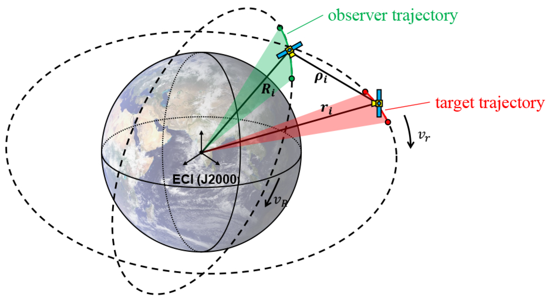
Recently, the passive optical sensors deployed on space platforms have become a promising alternative for space tracking as it eliminates the restrictions on weather and terrain compared with the ground-based telescope. Space platforms have shorter distances to targets than ground facilities, and the apparent angular velocity from the observer to the target may be higher. Therefore, the space-based optical measurement is a typical scenario of too short arcs and has been chosen as the focus of this paper.

Initial orbit determination from optical measurements, otherwise known as angle-only IOD, is built upon two-body dynamics. Previous approaches tackled the IOD problem in different ways, mainly falling into two categories: direct methods and iterative-based techniques [2]. Given the geometric relations and fundamental dynamical assumptions, the direct methods construct and solve polynomial equations to obtain feasible orbits. With three-angle observations, Laplace and Gauss [3] achieved the estimation for the orbits of natural celestial bodies. Together with their work, a number of articles detailing the theory and application of these two methods have been published. Rather than using the Lagrange’ formula for the line-of-sight (LOS) vector and its derivative as the classical Laplace’s method, Ref. [4] chose higher order unit sphere-constrained interpolation to build the terms of polynomial equations and achieved significant performance improvements. In addition, based on Charlier’s theory, [5,6] provides a geometric interpretation of the occurrence of multiple solutions in direct methods, which is useful to understand when there are multiple solutions and where they are located. With the advent of the space age, computer-based algorithms with iterative nature have been developed. Iterative algorithms make guesses on some dynamic terms and have them modified by an iterative process. When the residual between the propagated measurements and the actual ones approaches zero, an orbit solution is obtained. The double-r method, proposed in [3], iterates around estimates of the magnitudes of the radius vectors, while Gooding’s algorithm [7] implements its iteration based on slant ranges of two measurement epochs. Recently, three techniques of $L_n$, $J_n$[8], and $P_n$ [9] are also proven to be candidates for the iterative IOD methods. Many reviews and comparisons of these classical methods are made [2,10]. It shows that every method has its scope of application, but there are cases that do not perform particularly well under any IOD approach.

Moreover, to deal with the problem of TSAs, there are some works that have been proposed recently. One of the most valuable methods is the one based on the constrained admissible region (AR). Milani et al. [1,11] introduced the attributable, containing all the significant information in short arc measurements, and constrained all the possible orbit solutions on a ($r,\dot{r}$) compact subset, known as the admissible region. Motivated by this significant contribution, Tommei [12] first used the admissible region, a definition of heliocentric astronomy, to address the track association problem of space debris orbiting the Earth and then perform a full orbit determination based on the associated data. DeMars [13] developed a probabilistic approach based on an admissible region to ensure the inspiring accuracy of IOD, only with the angle rate information added. Furthermore, considering the uncertainty on the solution within the admissible region, Pirovano [14] refers to the multiple orbits that comply with the TSA observations as an orbit set (OS), and combines two or more OSs to determine a common solution [14]. On the other hand, the method based on the conservation laws of Kepler’s problem has recently been investigated by Gronchi et al. for the computation of preliminary orbits. The authors derived algebraic equations using the first integrals of Kepler’s motion, and developed the elimination step based elementary calculations, resulting in a univariate polynomial equation of degree 9 in the radial distance [15,16,17,18]. The Kepler Integral (KI) method has been tested with both synthetic and real data of asteroids and can enable the linkage of VSAs even when they are separated in time by a few years [19].

Evolutionary algorithms (EAs) are a class of population-based heuristic search approaches that have been successfully applied in many engineering fields to solve various optimization problems [20,21]. Recently, because of its ease of implementation and guaranteed convergency, some researchers have also introduced evolutionary algorithms to solve IOD problems. Ansalone [22] is the first one using an evolutionary algorithm to deal with the TSA problem. Using slant distances of two observation times as optimization variables, the author performed orbit determination for every guess in the framework of the Lambert problem. The simulation experiment on space-based observation of 60 s arcs achieved superior performance. Following this, Hinagawa[23] transferred the technique to the IOD of geostationary satellites based on true observation from the ground telescope, further verifying the effectiveness of EA-based IOD. In addition, there exist studies of directly using orbital elements as optimization variables [24]. This approach avoids the Lambert solver’s computation consumption that Ansalone used.

The solving process of EAs is essentially an iterative searching process within the parameter space. Individuals in the parameter space are mapped to the fitness space by a cost function and then guided to evolve to a better location based on the information feedback from the fitness landscape. Thus, the implemented optimization method and the understanding of the fitness space are the keys to a good result. Due to the sparsity of observations and noise interference, the IOD optimization problem may have more than one best solution and hence is a multimodal problem, which is ignored by current works. In this paper, we introduce an improved differential evolution (DE) algorithm to solve the IOD problem from the perspective of multimodal optimization. The main contribution of this paper is as follows:

1.

In this paper, based on the analysis of IOD parameter space, a multimodal optimization strategy for IOD is proposed for the first time to enhance the success rate and the accuracy of the IOD solution;

2.

A multimodal differential evolution with niching, convergence detection, and archiving strategy, termed as DE-NBA, is proposed in this paper. Considering the importance of evolution state for the computational resource allocation, a convergence detector based on the Boltzmann Entropy is designed as a component of the DE-NBA;

3.

The proposed method in this paper achieves competitive performance in 20 problems of the CEC2013 multimodal competition, against 11 common algorithms, which verifies its ability for a multimodal problem;

4.

Three space-based scenarios of a 60 s short arc observation are simulated to test the proposed multimodal algorithm for initial orbit determination. With 100 Monte Carlo experiments, the proposed algorithm is compared with the classical Gauss method, the single-mode DE, and the recent multimodal FBK-DE. The results show the applicability and accuracy of our method. Moreover, performance tests under different noise levels are conducted to estimate the availability of the proposed IOD method in practice.

The rest of this paper is organized as follows: Section 2 introduces the formulations of the EA-based IOD, and illustrates the multimodal phenomenon of IOD optimization problems. The developed DE-NBA is described component-by-component in Section 3. Two experiment cases and their results are presented in Section 4. The discussion and conclusions are shown in Section 5 and Section 6, respectively.

2. Related Works

2.1. Angle-Only IOD Problem

An observation scenario of the space-based satellite toward others is shown in Figure 1, which provides tracklets of too short arc measurements. In the earth centered inertial (ECI) frame, the position of the observer, the target, and the center of the earth forms a triangular relationship. Given a few pairs of angle information at different epochs within one observation span, the state of target is expected to be estimated as accurately as possible. With the measurements of $\{t_i,{\alpha }_i,{\delta }_i,i=1,2,\cdots ,n\}$, where $({\alpha }_i,{\delta }_i)$ are the right ascension and declination at the time of $t_i$, we can express the target position using the following relations:

$$\begin{array}{cc}\hfill \overrightarrow{{\mathit{r}}_{\mathit{i}}}& =\overrightarrow{{\mathit{R}}_{\mathit{i}}}+{\rho }_i\overrightarrow{{\mathit{l}}_{\mathit{i}}},\hfill \\ \hfill \overrightarrow{{\mathit{l}}_{\mathit{i}}}& ={(cos{\delta }_{i}cos{\alpha }_i,cos{\delta }_{i}sin{\alpha }_i,sin{\delta }_i)}^T,\hfill \end{array}$$

(1)

where $\overrightarrow{{\mathit{r}}_{\mathit{i}}}$ is the geocentric position vector of the target; $\overrightarrow{{\mathit{R}}_{\mathit{i}}}$ is the geocentric position vector of the observer; ${\rho }_i$ presents the slant range between the observer and the target; and $\overrightarrow{{\mathit{l}}_{\mathit{i}}}$ is the unit vector of the line of sight (LOS) derived by an angular measurement.

2.2. Evolutionary Algorithm Based IOD

For building an optimization IOD task, there are mainly two steps:

1.

Specify the variables for optimization based on the measurement types and construct the cost function based on the underlying principles of dynamics and kinematics;

2.

Select an evolutionary algorithm to explore and exploit the fitness landscape of the IOD problem, and then evolve for an orbit solution by enforcing the cost function approaches zero.

Different choices of variables correspond to different optimization formulas. Under the angle-only measurement scenario, the slant range ${\rho }_i$ in the Equation (1) is unknown. A direct implementation of the EA-based IOD is taking ${\rho }_i$ as the optimization variable so that the full orbit representation of the target can be acquired. As implemented in [22], following the solution obtained by the Lambert solver, the calculation procedure can propagate the candidate orbit to the measurement epochs and obtain a corresponding LOS set. Finally, a cost function is formulated as the residual between the propagated and true observation, shown in Equation (2).

$$f(X)=\prod _{i=2}^{n-1}(\overrightarrow{{\mathit{l}}_{\mathit{i}}}·\overrightarrow{{\mathit{l}}_{\mathit{i}}^{{}^{\prime }}})$$

(2)

where X represents the individual in the parameter space, consisting of slant ranges in two epochs, (${\rho }_1,{\rho }_n$); $\overrightarrow{{\mathit{l}}_{\mathit{i}}}$ and $\overrightarrow{{\mathit{l}}_{\mathit{i}}^{{}^{\prime }}}$ are the true and the propagated LOS, respectively. The result of Equation (2) implies the deviation of X from the true value. It can be seen from Figure 2a that the larger the result, the larger the position deviation.

In addition, an object’s orbit can be entirely determined by the Keplerian orbital elements ($a,e,i,\mathsf{\Omega },\omega ,M$), where a is the semi-major axis, e is the eccentricity, i is the inclination, $\mathsf{\Omega }$ is the right ascension of the ascending node, $\omega$ is the argument of periapsis, and M is the mean anomaly. The slant range ${\rho }_i$ is defined in terms of the ($a,e,M$) by:

$$\begin{array}{cc}\hfill r_i& =a(1-ecos{E}_i),\hfill \\ \hfill Z_i& =arccos(\frac{\overrightarrow{{\mathit{R}}_{\mathit{i}}}·\overrightarrow{{\mathit{l}}_{\mathit{i}}}}{R_i{l}_i}),\hfill \\ \hfill {\rho }_i& =\sqrt{r_i^2-R_i^2{sin}^2{Z}_i}-R_{i}cos{Z}_i,\hfill \end{array}$$

(3)

where $Z_i$ represents the angle between the line-of-sight vector and the target geocentric vector.

Substituting the resulting ${\rho }_i$ into Equation (1), the geocentric position vector of the target $\overrightarrow{{\mathit{r}}_{\mathit{i}}}$ can be obtained by combining the knowledge of the observer location and measured LOS. As shown in Figure 2b, two virtual arcs can be constructed using the calculated $\overrightarrow{{\mathit{r}}_{\mathit{i}}}$ and the selected $X=(a,e,M)$, respectively. A cost function implemented in [25] is given by:

$$\begin{array}{cc}\hfill E& =M+esinE,TA=arctan(\frac{\sqrt{1-e^2}sinE}{cosE-e}),\hfill \\ \hfill f(X)& ={({\displaystyle \sum _{j=1}^{n-1}}{\displaystyle \sum _{k=j+1}^n}{(T{A}_k-T{A}_j-arccos(\frac{\overrightarrow{r_k}·\overrightarrow{r_j}}{r_k{r}_j}))}^2)}^{1/2},\hfill \end{array}$$

(4)

where $T{A}_k,T{A}_j$ represent the true anomaly of different epochs, and they are calculated based on the mean anomaly M of different times. M first converts to the eccentricity anomaly E by an iteration method; then, $TA$ can be obtained combined with the eccentricity e. If the candidate X is compatible with the measurements, the cost function will become zero.

2.3. Analyses on Fitness Landscape of the IOD Problem

When transforming the IOD into an optimization task, an interesting question is what form the fitness space takes. The fitness landscape behind the typical scenarios, where the observer is in low Earth Orbit (LEO), the target respectively in the low Earth Orbit, medium Earth Orbit (MEO), and geostationary Earth Orbit (GEO), is investigated in this section. The underlying cost function adopts the form of Equation (4), and the parameter space takes the same setup as Section 4.2. Fixing ($e,M$) and M as the true value in turn, then the 1D and 2D fitness landscape can be obtained by sampling the remaining items.

We set a bound on the optimized parameter so that the target will not impact the Earth, seen as Equation (15), and the samples that violate the constraint will be penalized with an infinite value, which is shown as the gray areas of Figure 3. The visualization presentation of the fitness landscape shows that, although there is only one optimum in 1D fitness curves of all three scenarios, multiple minima exist in 2D fitness landscapes and have the depth of the same level, as shown in the dark blue part of the landscape contours.

Considering the IOD problem to be solved is a 3D optimization problem in this paper, the underlying fitness landscape will be more complex. When a single-modal evolutionary algorithm is used, the existence of multiple optima could pose difficulties to the optimization process and even serve to draw away an optimization algorithm from the true solution because the single-modal evolutionary algorithms seek one best solution at one time and are hard to escape from local optima.

3. Proposed Method

Motivated by the multimodal phenomena of the IOD problem of space-based measurement, this paper introduces an improved differential evolution algorithm with multimodal characteristics to solve the TSA challenge. Three functional components are implemented in the following sections, including the basic differential evolution driver, a coarse-to-fine niching strategy, and a convergence detector based on Boltzmann entropy.

3.1. Differential Evolution

Differential evolution (DE) is a powerful searching method for solving optimization problems over continuous space, which is widely used in a variety of engineering application. As a classical single-modal evolutionary algorithm, DE tries to evolve the population toward the optimum with the greedy strategy. Its implementation mainly includes four parts:

• Initialization. Given the lower bound, $l_j$, and upper bound, $u_j$, of the individual, the initial population, size of $NP$, are randomly sampled in the parameter space according to a uniform distribution, $U(l_i,u_j)$:

  $$\begin{array}{c}\hfill x_{i,j}(0)=l_j+U(l_j,u_j)\end{array}$$

  (5)

  where $x_{i,j}$ represents the j th dimensional value of the i th individual at g th generation; subscripts i and j are in the range $[1,NP]$ and $[1,D]$, where D represents the dimension of the problem.
• Mutation. The original DE generates offspring individuals by adding weighted reference vectors, made of the difference between two individuals, to a third.

  $$v_i(g)=x_{r1}(g)+F·(x_{r2}(g)-x_{r3}(g))$$

  (6)

  where the subscripts $r1,r2$ and $r3$ are randomly picked from {$1,2,3,\cdots ,NP$}∖{i} and mutually exclusive; the scale factor F weights the contribution of the difference vectors to control the mutation step.
• Crossover. After mutation, DE generally exchanges some components from $x_i$ and $v_i$ to form a trial vector $u_i$, which is the binomial crossover operation:

  $$u_{i,j}(g)=\left\{\begin{array}{cc}{v}_{i,j}(g)& ifrand\le CRorj=j_{rand}\\ x_{i,j}(g)& otherwise\end{array}\right.$$

  (7)

  where $CR$ represents the crossover rate, which is usually set to a fixed value lying in the range $[0,1]$; $j_{rand}$ is the dimension index, randomly selected from {$1,2,\cdots ,D$} to make sure that there must be one dimension where the value comes from $v_{i,j}$.
• Selection. The selection operator is utilized to choose the best individual from $x_i(g)$ and $u_i(g)$ into the next generation. It is given as follows:

  $$x_i(g+1)=\left\{\begin{array}{cc}{u}_i(g)& iff(u_i(g))orj=j_{rand}\\ x_i(g)& otherwise\end{array}\right.$$

  (8)

  where $f(·)$ represents the fitness function of the optimization problem.

In addition, given the changing fitness landscape in different problems and evolving stages, the adaptive adjustment strategy [26] of F and $CR$ is utilized in the optimization progress, shown in Equation (9). F and $CR$ are sampled from Gaussian distribution and Cauchy distribution, respectively. In addition, they are updated by maintaining a historical memory for successful F and $CR$, that is, every time the offspring generated by $F_i$ and $C{R}_i$ has better fitness than its paired solution, the $F_i$ and $C{R}_i$ will be recorded into $S_F$ and $S_{CR}$, respectively, shown in Equation (10):

$$\begin{array}{c}\hfill F=Cauchy({\mu }_F,0.1),CR=Gaussian({\mu }_{CR},0.1),\end{array}$$

(9)

$$\begin{array}{c}\hfill {\mu }_F=\frac{{\sum }_{i=1}^{|S_F|}{w}_i·S_{F,i}^2}{{\sum }_{i=1}^{|S_F|}{w}_i·S_{F,i}},{\mu }_{CR}=\sum _{i=1}^{|S_{CR}|}{w}_i·S_{CR,i},\end{array}$$

(10)

where $w_i$ represents the percentage of fitness improvement obtained by ith successful mutation to all fitness improvements.

Multimodal evolutionary algorithms with superior performance must find as many optima as possible in each iteration while keeping them evolving. Combining the above components, how to modify the DE for multimodal search capabilities becomes the focus in this paper. Following the works of the niching technique [27] and the convergence detection [28,29], we design two strategies to enhance the DE for solving the multimodal problem, which are described in Section 3.2 and Section 3.3.

3.2. Two-Layer Niching Method

Multimodal evolutionary algorithms seek to simultaneously locate and maintain a large number of global optima, which is heavily dependent on the population diversity. Niching techniques are one of the most widely used multimodal strategies, mainly including fitness sharing, crowding, speciation, clearing [30,31], and clustering [32]. Based on these niching techniques, recent DE variants (such as the CDE [33], SDE [34], NCDE, and NSDE [35]) have shown excellent performance in multimodal problems. Notably, many niching methods need to adjust parameters for various problems, and it has become a significant barrier in their application [27].

The Nearest-Better Clustering (NBC) [36] is a niching method that divides the population to form species that evolve simultaneously. It only needs one scalar parameter to control the sizes of various species, thus becoming popular in solving multimodal problems [37]. However, the traditional NBC cannot handle it well when the distribution of optima in the parameter space is uneven, that is, the distances between peaks vary greatly. Individuals who belong to different peak regions may be assigned to the same species. In this section, we propose a strategy of two-layer nearest-better clustering (TLNBC) to distinguish all peak regions and reasonably allocate resources to those areas, and its implementation is given in Algorithm Section 3.2.   

Algorithm 1 Two-layer nearest-better-clustering with minimize size (TLNBC)

Input: Population: P; Minimal number of individuals in various species: minsize; Scalar factor: ${\alpha }_1$, ${\alpha }_2$.

Output: Species: S.

1: Divide P using the big ${\alpha }_1$: $S_1\leftarrow mNBC(P,minsize,{\alpha }_1)$.

2: Set individuals better than others in the same species as seeds, $see{d}_i$.

3: Perform local search around $see{d}_i$.

4: Set the number of all individuals as N.

5: Set the number of species as $N_{s1}$

6: Calculate a modest capacity of species:$c=⌊N/N_{s1}⌋$

7: for each species $s_i$ in $S_1$ do

8:    $\delta =nums(s_i)-c$

9:    if $\delta >0$ then

10:      Discard the worst $\delta$ individuals in $s_i$ by fitness value.

11:    else

12:      Sample $\left|\delta \right|$ individuals by $N(see{d}_i,0.1)$ and add them to $s_i$.

13:    end if

14: end for

15: if ($N-c\times N_{s1})>0$ then

16:    Select ($N-c\times N_{s1}$) species randomly, adding one individual to each species.

17: end if

18: Divide the updated P using the small ${\alpha }_2$: $S\leftarrow mNBC(P_{update},minsize,{\alpha }_2)$.

In detail, in order to obtain a discriminative clustering on peak regions, we perform NBC procedure twice. A coarse clustering is first performed in the population using a big scalar factor to determine the major peak regions. The size of the resulting species would be large, which may make different peaks overlap within the same species. The local optima in species are regarded as seeds of those areas. One local search [38] on the seeds is then performed to advance their dominance. Then, the size deformation (Lines 7–14) is made to balance the computation resources allocated to different peak regions, which enables the vast majority of potential regions to continue their exploration when some individuals enter a prematurely convergent state. Finally, the second mNBC is performed to obtain the highly recognizable peak species.

The primary component of TLNBC adopts the mNBC, an NBC variant proposed in [39], to identify the basin attraction. It enforces a constraint on the minimal number of individuals in species so that it enables basic mutation within every peak region. Algorithm 2 presents the details of the mNBC: the $\alpha$ controls the size of the resulting species adaptively, and the minsize gives the lower bound of number for species individual.   

Algorithm 2 Nearest-better clustering with minsize [39]

Input: Population: P; Minimal number of individuals in various species: minsize; Scalar factor: $\alpha$.

Output: Species: S.

1: Sort P by the fitness value in descending order.

2: Calculate the distances between each pair of individuals.

3: Create an empty tree T.

4: for each individual $x_i$ in P do

5:    Obtain the individual set $S_b$ in which each element is better than $x_i$.

6:    Find the nearest individual in $S_b$ to $x_i$, termed $x_{nb}$.

7:    Create an edge between $x_i$ and $x_{nb}$ and add it to T.

8: end for

9: Calculate the mean distance of all edges in T, termed ${\mu }_{dist}$.

10: for each $e_j$ in T do

11:    if $dist(e_j)>\alpha \times {\mu }_{dist}$ then

12:      Set $T_f$ to the subtree rooted at the follower individual of $e_j$.

13:      Set $T_r$ to the subtree containing the follower individual of $e_j$.

14:      if the node number of $T_f$ is more than minsizethe node number of $T_r$ is still more than minsize after $e_j$ is cut then

15:         Cut off $e_j$.

16:      end if

17:    end if

18: end for

19: S ← All independent subtrees that do not share edges with others.

3.3. Convergence Detection Based on Boltzmann Entropy

The multimodal algorithm seeks to locate and preserve as many optima as possible. Due to the asynchronous development levels in the different subregions of the fitness space, some high-potential individuals around one peak would be attracted to premature ones, resulting in the omission of optima in some subregions. A useful scheme is to divide the evolution into exploration and exploitation stages based on the behavior of the evolving population. In the exploration stage, the individuals tend to exchange information between niches to find more feasible regions. In the exploitation stage, the subregions focus on the inner-niches refinement to build more precise solutions. A strategy to distinguish evolving status is the convergence detection.

A good detector can efficiently identify the occurrence of the potential niches, both in any parameter and fitness space. This section proposes a convergence detection strategy based on the Boltzmann Entropy [40,41,42]. The traditional detector would respond to the convergence happening in the parameter or fitness space independently; one intuitive idea is whether one convergence indicator can simultaneously reflect parameter and fitness space changes. Algorithm 3 gives a procedure to implement coarse-to-fine convergence detection over all parameter dimensions.

Algorithm 3 Convergence detection for the population in the domain of distance and fitness

Input: Population: P; Scalar factor:$k_0$; Threshold: $ϵ$.

Output: Convergence flag: Go.

1: Create a historical record of BE value, S.

2: $Go\leftarrow FALSE$

3: while not reach the max generation do

4:    Construct a slice set of the heatmap based on the individual distribution in P using $k_0$.

5:    Calculate the absolute Boltzmann Entropy $S_A$ and add it to S.

6:    $c_1$ = mean(last $g_1$ elements of S), $c_2$ = mean(last $g_2$ elements of S).

7:    if $\frac{|c_1-c_2|}{c_1}<ϵ$ then

8:      $Go\leftarrow TRUE$

9:    end if

10: end while

First, a slice set of the heatmap is built based on the individual distribution in the dimensions of parameter and fitness. The distance and fitness value domain is divided into a block diagram by the scalar parameter $k_i$. The number of individuals falling into blocks becomes the pixel value of the heatmap, which is shown in Figure 4.

It is apparent that $k_i$ controls the resolution of the ith heatmap in the slice set and accordingly decides the sensitivity of the convergence criterion. At the early evolving stage, individuals at most dimensions are random, we set the $k_i$ with initial value $\sqrt{N_{pop}}$, which is the square root of the numbers of the population; and the $k_i$ increases two as soon as the convergence is detected in the i th heatmap.

Second, a hierarchy-based approach [42] is adopted to compute the Boltzmann Entropy ($BE$) of those heatmaps for identifying the evolution stage of the population. The original BE calculation is expressed through two notions, namely macrostate and microstate. By determining the number of possible microstates (W) corresponding to the same macrostate, the BE value can be calculated with the following equation:

$$S=k_{B}log(W)$$

(11)

where $k_B$ is the Boltzmann constant ($=1.38\times {10}^{-23}$ J/K).

In [40,42], Gao et al. regard the abstract representation of an image as the macrostate, and all the possible images satisfying the patterns of the macrostate mask as the microstate. As shown in Figure 5, a hierarchical downsampling repeats until the image degenerates to a pixel. With the constraints on the minimum, maximum and mean for the underlying patch, every aggregated pixel in the nth level (macrostate unit) corresponds to $w_i$ microstates, and total ${\prod }_i{w}_i$ will be obtained in this level. By an inverse image reconstruction from the highest level to the lowest, we can obtain different relative BE value ($S_R$) using Equation (11), and the absolute BE value ($S_A$) equals the sum of all $S_R$.

Finally, a convergence criterion is set based on the change of resulting Boltzmann Entropy: after fixed generations for exploration in every evolving round, if the mean of $S_A$ in the last continuous two duration fluctuates within a limited range, it can be judged that convergence has been detected.

3.4. DE-NBA

Algorithm 4 shows the proposed DE algorithm, termed DE-NBA, based on the niching strategy, convergence detector, and a trick of external archive. The algorithm starts with the initialization of population. Due to the distribution of the first generation population is random, the algorithm divides the individuals into multiple species by the mNBC with a large scalar factor, ${\alpha }_1=2$. Then, a niche-level optimization strategy proposed in [26] is implemented in the DE-NBA. It decides whether the recombination occurs within the same niche or between the species by the probability $pr$, shown in Equation (13). In each population optimization, the individual with high-potential tends to exploit while the low potential individual is possible to explore:

$$P{V}_i=f_{i,ave}(f_{i,seed}-f_{i,ave})$$

(12)

$$p{r}_i=\frac{P{V}_i-P{V}_{min}}{P{V}_{max}-P{V}_{min}}$$

(13)

where $f_{i,ave}$ represents the average fitness in i th species, $f_{i,seed}$ represents the fitness of the seed of i th species, and $P{V}_i$ is the potential value of the current species, indicating the diversity of the corresponding subpopulation. $P{V}_{min}$ and $P{V}_{max}$ represent the minimum and maximum potential value among all species; the resulting $p{r}_i$ is the probability that decides whether the recombination occurs within the same species or between different species.

Once the convergence state is detected, the TLNBC performs coarse-to-fine niching and makes the optimized seeds archived. The archive, as the supporting individuals, will merge with the basis population into next evolution. Finally, the archive individuals will perform a local search to improve their accuracy. The whole computation resources are divided into two parts, one for the global optimization and another for the local search: the percentage is 7:3.

Algorithm 4 The Proposed DE-NBA

Input: P, $lb$, $ub$, $maxEval$, $minsize$, $maxArchive$, $k_0$, ${\alpha }_1$, ${\alpha }_2$, $maxLS$, $maxFES$.

Output:A.

1: Initiate the population P.

2: ${\mu }_F\leftarrow$ 0.5, ${\mu }_{CR}\leftarrow$ 0.5.

3: A ← [].

4: S ← mNBC(P, minsize, ${\alpha }_1$).

5: $g\leftarrow$ 1.

6: while numEval < maxLS do

7:    P ← DE(P, A, ${\mu }_F$, ${\mu }_{CR}$).

8:    Calculate the Boltzmann entropy $S_A$ and add it to the history record $S_{BE}$.

9:    if mod(g,20)==0 then

10:      if The convergence is detected then

11:         S ← TLNBC(P, minsize${\alpha }_1$, ${\alpha }_2$).

12:         Select the seeds among S into A.

13:         if nums(A)>$maxArchive$ then

14:           Drop out the oldest (nums(A)>$maxArchive$) elements in A.

15:         end if

16:      end if

17:    end if

18:    $g\leftarrow$$g+1$.

19: end while

20: while numEval < maxFES do

21:    A ← NelderMead(A).

22: end while

4. Results

The proposed differential evolution with multimodal property is firstly evaluated on the 2013 IEEE Congress on Evolutionary Computation Competition (CEC2013) on Niching Methods for Multimodal optimization [43], as shown in case study 1, to present its competitive performance against 11 multimodal evolutionary algorithms. Then, the effectivity of the proposed multimodal DE in the IOD of space based observation is verified when compared with classical Gauss method, single modal DE algorithm, and a state-of-the-art multimodal algorithm. In addition, we conducted a series of IOD experiments based on simulated observations at different noise levels, aiming to test the applicability of the proposed method.

4.1. Case Study 1

4.1.1. Experiments Protocol

The CEC2013 is a multimodal optimization competition, with an aim to build a unifying framework for evaluating niching methods. The 20 benchmark multimodal functions with different characteristics and levels of difficulty are included in CEC2013, which are shown in

Table 1. Benchmark test functions.

F	Name	D	Peak Height	No. Optima	Max. Func. Eval.
F1	Five-Uneven-Peak Trap	1	200.0	2	$5.0\times {10}^4$
F2	Equal Maxima	1	1.0	5	$5.0\times {10}^4$
F3	Uneven Decreasing Maxima	1	1.0	1	$5.0\times {10}^4$
F4	Himmelblau	2	200.0	4	$5.0\times {10}^4$
F5	Six-Hump Camel back	2	1.03163	2	$5.0\times {10}^4$
F6	Shubert	2	186.731	18	$2.0\times {10}^5$
F7	Vincent	2	2709.0935	36	$2.0\times {10}^5$
F8	Shubert	3	1.0	81	$4.0\times {10}^5$
F9	Vincent	3	−2.0	216	$4.0\times {10}^5$
F10	Modified Rastrigin	2	0	12	$2.0\times {10}^5$
F11	Composition Function 1	2	0	6	$2.0\times {10}^5$
F12	Composition Function 2	2	0	8	$2.0\times {10}^5$
F13	Composition Function 3	2	0	6	$2.0\times {10}^5$
F14	Composition Function 3	3	0	6	$4.0\times {10}^5$
F15	Composition Function 4	3	0	8	$4.0\times {10}^5$
F16	Composition Function 3	5	0	6	$4.0\times {10}^5$
F17	Composition Function 4	5	0	8	$4.0\times {10}^5$
F18	Composition Function 3	10	0	6	$4.0\times {10}^5$
F19	Composition Function 4	10	0	8	$4.0\times {10}^5$
F20	Composition Function 4	20	0	8	$4.0\times {10}^5$

. The source codes of the benchmark test functions can be downloaded from the CEC2013 special session on niching methods website (https://github.com/mikeagn/CEC2013 (accessed on 1 September 2022)). In these benchmark functions, the functions of F1 to F5 are simple functions, and the F6–F10 are functions which have a large number of global optima. Furthermore, function F7 contains a large gap between peaks. F11–F20 are the composition functions with many local peaks, among which F16–F20 are relatively high dimensional.

There are two metrics widely used in the multimodal optimization competition for performance comparison, the peak ratio (PR) and success rate (SR). All competition algorithms are run for a fixed number of rounds (NR). The PR represents the ratio of the number of peaks the algorithm (NPF) found to that of the processed problem (NPK) over all runs. When all peaks of a problem are found, it is called a successful run. The SR equals the number of success runs (NSR) divided by NR. The related formulations are as follows:

$$\begin{array}{cc}\hfill PR& =\frac{{\sum }_{i=1}^{NR}NP{F}_i}{NR·NPK},\hfill \\ \hfill SR& =\frac{NSR}{NR},\hfill \end{array}$$

(14)

Table 2. Parameters in DE-NBA.

Parameters	Values
maxGen	200 (D < 5)
	300 (D ≥ 5)
$k_0$	20
${\mu }_F$	0.5
${\mu }_{CR}$	0.5
minSize	5
${\alpha }_1,{\alpha }_2$	2, 1
maxLS	$0.3·maxFEs$

gives the parameter setups for the proposed algorithm. Because the number of global optima is unknown, we relate the individual number NP to the problem dimension. When the problem becomes complex, the number of explored populations increases to improve the probability of finding more optima. In detail, NP is determined based on the allowed number of evolution generation maxGen. When the dimension of problem D is less than 5, maxGen is set to 200, while the dimension is greater than 5, maxGen is set to 300, and the corresponding NP is equal to maxFES divided by maxGen.

During the optimized process, the population will experience multiple rounds of convergence. Before the procedure of convergence detection, the algorithm needs at least $k_0$ generations to drive the distinct species exploring for the local peaks. In the basic DE optimizer, given the capability of adaptive tuning of F and CR, we initiate the parameters ${\mu }_F$ and ${\mu }_{CR}$ with a 0.5 at the beginning of each convergence round.

Once the population converge to different peaks of fitness landscape, we adopt a coarse-to-fine TLNBC to find as many peaks as possible. The large scalar factor means the population tree is easily cut off for more niches, while the small value just obtains the opposite result. Thus, the first factor ${\alpha }_1$ in TLNBC is set to 2 to acquire a coarse niche set. The ${\alpha }_2$ is set to 1 for identifying different promising solution from the same basin of attraction. Finally, to achieve a balance between the exploration and exploitation, the maxFEs for local search on the archive is set to $0.3*MaxFEs$.

4.1.2. Results on DE-NBA

In this section, DE-NBA is first performed 50 times on CEC2013 benchmark problems. The PRs and SRs in five levels of accuracy $ϵ$ = $\{1\times {10}^{-1},1\times {10}^{-2},1\times {10}^{-3},1\times {10}^{-4},$$1\times {10}^{-5}\}$ are shown in

Table 3. PRs and SRs of proposed algorithm on 20 problems at five different accuracy levels.

$\mathit{ϵ}$	${\mathit{F}}_1(1\mathit{D})$		${\mathit{F}}_2(1\mathit{D})$		${\mathit{F}}_3(1\mathit{D})$		${\mathit{F}}_4(2\mathit{D})$		${\mathit{F}}_5(2\mathit{D})$
	$\mathit{PR}$	$\mathit{SR}$	$\mathit{PR}$	$\mathit{SR}$	$\mathit{PR}$	$\mathit{SR}$	$\mathit{PR}$	$\mathit{SR}$	$\mathit{PR}$	$\mathit{SR}$
$1\times {10}^{-1}$	1.000	1.000	1.000	1.000	1.000	1.000	1.000	1.000	1.000	1.000
$1\times {10}^{-2}$	1.000	1.000	1.000	1.000	1.000	1.000	1.000	1.000	1.000	1.000
$1\times {10}^{-3}$	1.000	1.000	1.000	1.000	1.000	1.000	1.000	1.000	1.000	1.000
$1\times {10}^{-4}$	1.000	1.000	1.000	1.000	1.000	1.000	1.000	1.000	1.000	1.000
$1\times {10}^{-5}$	1.000	1.000	1.000	1.000	1.000	1.000	1.000	1.000	1.000	1.000
$\mathit{ϵ}$	${\mathit{F}}_{\mathbf{6}}(\mathbf{2}\mathit{D})$		${\mathit{F}}_{\mathbf{7}}(\mathbf{2}\mathit{D})$		${\mathit{F}}_{\mathbf{6}}(\mathbf{3}\mathit{D})$		${\mathit{F}}_{\mathbf{7}}(\mathbf{3}\mathit{D})$		${\mathit{F}}_{\mathbf{8}}(\mathbf{2}\mathit{D})$
	$\mathit{PR}$	$\mathit{SR}$	$\mathit{PR}$	$\mathit{SR}$	$\mathit{PR}$	$\mathit{SR}$	$\mathit{PR}$	$\mathit{SR}$	$\mathit{PR}$	$\mathit{SR}$
$1\times {10}^{-1}$	1.000	1.000	0.960	0.280	0.955	0.000	0.831	0.000	1.000	1.000
$1\times {10}^{-2}$	1.000	1.000	0.930	0.060	0.952	0.000	0.675	0.000	1.000	1.000
$1\times {10}^{-3}$	1.000	1.000	0.927	0.040	0.952	0.000	0.649	0.000	1.000	1.000
$1\times {10}^{-4}$	1.000	1.000	0.914	0.020	0.942	0.000	0.630	0.000	1.000	1.000
$1\times {10}^{-5}$	1.000	1.000	0.903	0.000	0.088	0.000	0.621	0.000	1.000	1.000
$\mathit{ϵ}$	${\mathit{F}}_{\mathbf{9}}(\mathbf{2}\mathit{D})$		${\mathit{F}}_{\mathbf{10}}(\mathbf{2}\mathit{D})$		${\mathit{F}}_{\mathbf{11}}(\mathbf{2}\mathit{D})$		${\mathit{F}}_{\mathbf{11}}(\mathbf{3}\mathit{D})$		${\mathit{F}}_{\mathbf{12}}(\mathbf{3}\mathit{D})$
	$\mathit{PR}$	$\mathit{SR}$	$\mathit{PR}$	$\mathit{SR}$	$\mathit{PR}$	$\mathit{SR}$	$\mathit{PR}$	$\mathit{SR}$	$\mathit{PR}$	$\mathit{SR}$
$1\times {10}^{-1}$	1.000	1.000	0.997	0.980	0.963	0.780	1.000	1.000	1.000	1.000
$1\times {10}^{-2}$	0.996	0.980	0.997	0.980	0.880	0.360	0.666	0.000	0.730	0.000
$1\times {10}^{-3}$	0.990	0.940	0.997	0.980	0.876	0.360	0.666	0.000	0.730	0.000
$1\times {10}^{-4}$	0.986	0.920	0.997	0.980	0.873	0.340	0.666	0.000	0.730	0.000
$1\times {10}^{-5}$	0.813	0.200	0.985	0.900	0.696	0.000	0.666	0.000	0.512	0.000
$\mathit{ϵ}$	${\mathit{F}}_{\mathbf{11}}(\mathbf{5}\mathit{D})$		${\mathit{F}}_{\mathbf{12}}(\mathbf{5}\mathit{D})$		${\mathit{F}}_{\mathbf{11}}(\mathbf{10}\mathit{D})$		${\mathit{F}}_{\mathbf{12}}(\mathbf{10}\mathit{D})$		${\mathit{F}}_{\mathbf{12}}(\mathbf{20}\mathit{D})$
	$\mathit{PR}$	$\mathit{SR}$	$\mathit{PR}$	$\mathit{SR}$	$\mathit{PR}$	$\mathit{SR}$	$\mathit{PR}$	$\mathit{SR}$	$\mathit{PR}$	$\mathit{SR}$
$1\times {10}^{-1}$	0.996	0.980	0.517	0.000	0.003	0.000	0.000	0.000	0.000	0.000
$1\times {10}^{-2}$	0.666	0.000	0.477	0.000	0.003	0.000	0.000	0.000	0.000	0.000
$1\times {10}^{-3}$	0.666	0.000	0.477	0.000	0.003	0.000	0.000	0.000	0.000	0.000
$1\times {10}^{-4}$	0.666	0.000	0.477	0.000	0.003	0.000	0.000	0.000	0.000	0.000
$1\times {10}^{-5}$	0.666	0.000	0.400	0.000	0.003	0.000	0.000	0.000	0.000	0.000

. Furthermore, to better evaluate the performance of DE-NBA, 11 popular multimodal algorithms, such as the CDE [33], SDE [34], NCDE, NSDE [35], self-CCDE, self-CSDE [44], MOMMOP [45], LoICDE, LoISDE [46], PNPCDE [47], and recently FBK-DE [39], are selected to solve the same problems. Figure 6 gives the visualization results at the accuracy level $ϵ=1\times {10}^{-4}$ for comparison, which are commonly adopted in multimodal optimization competition [39,47].

Table 4. Statistical results of different algorithms’ performance on the benchmark problems over the accuracy level $ϵ=1\times {10}^{-4}$.

Algorithm	20 Benchmark Problems			15 Benchmark Problems
	PR (Mean)	PR (Std)	Rank	PR (Mean)	PR (Std)	Rank
CDE	0.45030	0.46271	6.35	0.58926	0.45410	5.46
SDE	0.26705	0.30990	8.85	0.33506	0.33143	9.13
NCDE	0.61390	0.32733	3.75	0.68420	0.33915	4.20
NSDE	0.27860	0.32053	8.25	0.32733	0.35910	8.93
self-CCDE	0.67605	0.33365	3.45	0.80926	0.24084	3.00
self-CSDE	0.48255	0.38003	7.20	0.63466	0.31061	6.40
MOMMOP	0.78035	0.27881	2.05	0.90713	0.15182	1.66
LoICDE	0.58245	0.36893	4.80	0.69920	0.33924	4.53
LoISDE	0.23015	0.29876	9.10	0.27253	0.33535	9.60
PNPCDE	0.50005	0.42057	5.95	0.65693	0.36515	4.73
FBK-DE	0.82990	0.20135	2.05	0.90826	0.15951	2.40
DE-NBA	0.74420	0.35680	2.90	0.91586	0.13154	1.60

The best PR and Rank are marked in bold in this table.

shows the statistical results of these multimodal optimization algorithms in all 20 problems and the first 15 problems. Notably, the recently compared results are from their corresponding papers, and the results of other algorithms are still from these papers.

It can be seen from Table 3 that DE-NBA presents stable performance in most lower-dimensional functions except for $F6(3D)$ at the $1\times {10}^{-5}$ accuracy level. On the first five problems, DE-NBA finds all solutions. On F6–F10, DE-NBA locates almost peak areas, and gets close to most peaks of the problems. In addition, when dealing with the composition problems, DE-NBA obtains good performance in the first F11–F15. As the problem dimension gradually increases, the performance of DE-NBA continues to deteriorate and eventually fails in the 10D and 20D problems.

Figure 6 shows the performance of the compared algorithms over accuracy level of $1\times {10}^{-4}$. Figure 6a presents a PR heatmap of 12 algorithms on 20 benchmark problems. The higher the PR value, the more efficient the corresponding algorithm is. It can be seen that the MOMMOP, FBK-DE, and our DE-NBA outperform the other nine algorithms. It is worth noting that solving high-dimensional multimodal problems is a real challenge for most EA-based algorithms. In the last three high-dimensional problems (F18, F19, and F20), DE-NBA performs the worst of the top three algorithms. Figure 6b illustrates the PR distribution of algorithms over the first 15 benchmark problems through a boxplot. The algorithms of the first three did not change, but the ranking changed, the DE-NBA won the first place. A more statistical result can be seen in Table 4, among which the average values and the standard deviations of PR are calculated on all 20 problems and on the first 15 problems, respectively. In addition, for each problem, each algorithm obtains a ranking based on its own results from the best to the worst. The rank column in Table 4 is the mean rank in the benchmark problems. From Table 4, it can be seen that DE-NBA achieves the third over 20 problems, and performs the best over the first 15 problems. Thus, the proposed DE-NBA has more significant potential to solve the lower-dimensional problems than the other problems.

4.2. Case Study 2

To present the superior performance of the proposed multimodal DE for IOD, we simulated three scenarios of space-based measurement in a two-body model. Specifically, the observer satellite is placed on the lower earth orbit, with the semi-major axis (a) of 6975.515 km, inclination (i) of $98.{137}^{\circ }$, argument of perigee ($\omega$) of $258.{759}^{\circ }$, right ascension of the ascending node ($\mathsf{\Omega }$) of $120.{968}^{\circ }$, and eccentricity (e) of 0.000253. Three targets are placed in the LEO, MEO, and GEO, and their orbit elements are listed in

Table 5. Instantaneous orbit elements of targets and space-based observation platform.

NORD Number	a/km	e	$\mathit{M}/{(}^{\circ })$	$\mathit{i}/{(}^{\circ })$	$\mathit{\Omega }/{(}^{\circ })$	$\mathit{\omega }/{(}^{\circ })$
21989	43,054.848	0.0082251	208.304	12.915	33.531	286.302
29422	11,762.622	0.440567	8.376	38.770	282.977	189.438
29444	7301.248	0.006782	104.893	64.940	184.440	156.585
observer	6975.515	0.000253	213.112	98.137	120.968	258.759

.

In this paper, we estimate the orbit states using two optimized processes to obtain a complete solution to the IOD problem. In the first stage, the $(a,e,M)$ of Keplerian elements are chosen as the optimization variables of a multimodal problem, the cost function follows the form of Equation (4), and the core optimized algorithm is the proposed DE-NBA. With the best result from the stage one, another problem that searches the $(i,\omega ,\mathsf{\Omega })$ space for optima is easy to be solved. We choose a basic DE to perform the second optimized process, and the underlying cost function is Equation (2).

The optimized domains of the six elements used in this paper are listed in

Table 6. The variable domain of the IOD optimization problem.

Parameter	$\mathit{a}/$km	e	$\mathit{M}/{(}^{\circ })$	$\mathit{i}/{(}^{\circ })$	$\mathit{\omega }/{(}^{\circ })$	$\mathit{\Omega }/{(}^{\circ })$
Domain	6400–50,000	0–1	0–360	0–180	0–360	0–360

.

It is well known that the searching region would be reduced to a tight area if there were constraints on optimized parameters, which could facilitate an optimization algorithm’s accuracy and convergence speed. However, in the IOD optimization problem, the detected target is usually uncooperative and no prior knowledge are available, thus this paper only chooses to use the universal rule that the Earth-orbiting satellite would not crash into the Earth to constraint the variable domain, seen as Equation (15):

$$a(1-e)>r_E$$

(15)

where $r_E$ is the radius of Earth (=6371.004 km).

Finally, the criterion that evaluates the applicability and the accuracy of compared methods in IOD is given here. In the IOD problem, the precision of the track surface is slightly better than the precision of the track, and Wu [48] pointed out that the a is the most important term in the orbit calculation. The deviation percentage between the estimated and the true a is defined as Equation (16). A deviation threshold that needs to be mentioned is 0.01, and its underlying IOD solution is considered valuable for orbit improvement and prediction:

$$per=\frac{|a_{estimated}-a_{true}|}{a_{true}}$$

(16)

4.2.1. Simulated Test in Three Observation Geometries

To simulate the observation of the too short arc, the observation duration is set to 60 s, and the data sampling rate is 1 Hz. With a series of angle measurements, $\{t_i,{\alpha }_i,{\delta }_i,$$i=1,2,\dots ,60\}$, a classical Gauss’ method, single-modal DE, FBK-DE, and the proposed DE-NBA perform 100 times of IOD to analyze their performance. Given a threshold of deviation percentage, when the bias of semi-major axis is less than the threshold, it is considered a successful IOD.

Figure 7 shows the cumulative distribution of the success percentage as a function of the deviation threshold under three scenarios. EA-based IOD methods achieve feasible solutions in all scenarios, which proves their applicability to space-based IOD. In the LEO-LEO and LEO-MEO, Gauss’s method cannot obtain a reasonable solution, accordingly, we would not include their solutions in the following statistical results; in the LEO-GEO, the best IOD score implies the effectivity of Gauss’s method when dealing with significant distance observations.

In the LEO-LEO scenario, when the threshold is set to 0.01, the success percentage of DE, FBK-DE, and DE-NBA are 0.61007, 1, and 0.68987, respectively, which is shown in Figure 7a. The distribution of orbit elements after 100 runs is depicted in Figure 8, and the statistical results, including the mean, medium, and the best solution, are given in

Table 7. Statistical results of IOD for LEO.

		a	e	i	$\mathit{\Omega }$	$\mathit{\omega }+\mathit{M}$
True Value		7301.2500	0.006782	64.9400	184.4400	261.4780
Mean	DE	7371.8598	0.004310	64.5728	184.9079	282.7048
	FBK-DE	7241.0961	0.013660	65.1246	184.4110	242.7694
	DE-NBA	7310.4451	0.011981	64.8887	184.5468	263.2991
Median	DE	7351.6734	0.002859	64.7453	184.5421	276.8380
	FBK-DE	7240.7807	0.013696	65.1400	184.3376	242.6761
	DE-NBA	7314.6335	0.008235	64.9355	184.4426	264.1487
Best	DE	7299.6539	0.007053	64.9550	184.4234	260.9705
	FBK-DE	7251.6090	0.012427	65.1008	184.3621	246.0988
	DE-NBA	7301.2500	0.006782	64.9327	184.4571	261.4704

The numbers closest to the truth in this table is marked in bold.

, which shows that the solution from DE-NBA is closer to the true one.

In the LEO-MEO scenario, when the threshold is set to 0.01, the success percentage of DE, FBK-DE, and DE-NBA are 0.10045, 0, and 0.60951, respectively, which is shown in Figure 7b. The distribution of orbit elements after 100 runs is depicted in Figure 9, and the statistical results, including the mean, medium, and the best solution, are given in

Table 8. Statistical results of IOD for MEO.

		a	e	i	$\mathit{\Omega }$	$\mathit{\omega }+\mathit{M}$
True Value		11,762.6220	0.440567	38.7700	282.9770	197.8140
Mean	DE	11,728.4160	0.438026	37.5410	281.0717	65.9212
	FBK-DE	11,951.2230	0.447132	37.2554	281.1395	216.2102
	DE-NBA	11,903.6150	0.445261	36.9671	280.1571	240.3982
Median	DE	11,359.6020	0.426160	38.0860	282.3972	155.7165
	FBK-DE	11,952.4700	0.447170	38.0211	282.4037	215.4260
	DE-NBA	11,770.6810	0.440850	37.8104	282.0987	202.7673
Best	DE	11,742.3580	0.439826	34.4353	277.7391	200.1070
	FBK-DE	11,913.5470	0.445826	38.5729	283.0061	211.3375
	DE-NBA	11,762.6220	0.440567	37.0898	281.0944	199.2696

The numbers closest to the truth in this table is marked in bold.

, which shows the solution from DE-NBA is closer to the true one.

In the LEO-GEO scenario, when the threshold is set to 0.01, the success percentage of Gauss, DE, FBK-DE, DE-NBA are 1, 0.88851, 0.34946, and 0.99151, respectively, which is shown in Figure 7c. Gauss’s method outperforms over all EA-based methods, and its performance is consistent. We depict the orbit element distribution of EA-based methods after 100 runs in Figure 10, and give statistical results of all compared approaches, include the mean, medium, and the best solution in

Table 9. Statistical results of IOD for GEO.

		a	e	i	$\mathit{\Omega }$	$\mathit{\omega }+\mathit{M}$
True Value		43,054.8480	0.008251	12.9150	33.5310	134.6060
Mean	DE	42,515.1150	0.011168	27.6340	139.9489	71.3651
	Gauss	43,054.8507	0.008251	12.9149	33.5309	134.6060
	FBK-DE	44,670.7730	0.038216	45.0654	207.9977	136.0535
	DE-NBA	42,215.8930	0.007213	33.2929	157.1196	51.8456
Median	DE	42,786.1980	0.005053	10.7424	65.6158	164.7784
	Gauss	43,054.8507	0.008251	12.9149	33.5309	134.6060
	FBK-DE	43,772.6520	0.020423	34.5762	276.3293	231.7916
	DE-NBA	42,957.1240	0.007216	15.7868	83.5302	136.1209
Best	DE	43,028.7560	0.005504	33.8258	286.1405	237.6507
	Gauss	43,054.8507	0.008251	12.9149	33.5309	134.6060
	FBK-DE	43,096.8900	0.008507	41.2641	77.1285	94.3451
	DE-NBA	43,052.7330	0.008226	14.0889	318.5244	208.0637

The numbers closest to the truth in this table is marked in bold.

. It can be seen that the solution of DE-NBA is the best one within the EA-based methods, but Gauss’s method ranks first among all metrics. One promising finding is that the best solution obtained by the DE-NBA is very close to that of Gauss’s method, indicating that the DE-NBA has a similar significant performance as Gauss’s method in the LEO-GEO scenario.

4.2.2. Performance Test in Different Levels of Noise

With the aim of investigating the robustness of the proposed method against noise, this section tests the performance of the proposed DE-NBA under nine levels of noise, $\sigma =\{1\times {10}^0,1\times {10}^{-1},1\times {10}^{-2},1\times {10}^{-3},1\times {10}^{-4},1\times {10}^{-5},1\times {10}^{-6},1\times {10}^{-7},1\times {10}^{-8}\}\backslash {(}^{\prime \prime })$. The generation of noise measurement follows the procedure used in [22]. First, the noiseless LOS vectors, l, are rotated about the axis $h=(l\times k_i)/|l\times k_i|$ by an angle $\alpha$, where $k_i$ is the unit vector of the inertial reference frame, $\alpha$ is sampled from a Gaussian distribution with the deviation standard ${\sigma }_i$. Then, the second rotation rotates the first result of an angle $\beta$ about the l axis, where $\beta$ is obtained from a uniform distribution between 0 and $2\pi$.

In this experiment, the proposed DE-NBA has run for 50 times to test its performance under different noise levels. Figure 11 shows the variation in the success percentage of IOD in different scenarios. When the threshold is 0.01, if the corresponding success percentage exceeds 0.5, it can be regarded that the algorithm can deal with this level of noise. In detail, in the LEO-LEO scenario, as shown in Figure 11a, the algorithm cannot achieve good results in the noise level of $\{1\times {10}^0,1\times {10}^{-1}\}$; in the LEO-MEO scenario, as shown in Figure 11b, the algorithm cannot achieve good results in the noise level of $\{1\times {10}^0,1\times {10}^{-1},1\times {10}^{-2}\}$; in the LEO-GEO scenario, as shown in Figure 11c, the algorithm cannot achieve good result in the noise level of $\{1\times {10}^0,1\times {10}^{-1},1\times {10}^{-2},1\times {10}^{-3}\}$.

5. Discussion

In Section 4, two experiments are designed to assess the performance of the proposed algorithm. The first experiment is conducted to evaluate the performance of the proposed multimodal evolution algorithm on the CEC2013 multimodal benchmark problems. The results are described in Section 4.1. The second experiment is designed to assess the accuracy and applicability of the IOD method which employs the proposed multimodal evolution algorithm as the core component. The test results are shown in Section 4.2. In this section, the two experimental results are discussed.

5.1. Competition Analysis of CEC 2013

Finding and maintaining global or local solutions as much as possible in the evolutionary process is a key step in an efficient multimodal optimization algorithm, and the SR and PR are usually used as evaluation criteria in the experiments. On the CEC2013 multimodal optimization competition, the performance of DE-NBA ranks third in 20 optimization problems; the first is FBK-DE, and the second is MOMMOP.

It is worth noting that the DE-NBA finds all the peaks on optimization problems F1–F6 and F10, and locates almost all the peak regions in problems F7–F10. Compared with FBK-DE, the PR improvement of DE-NBA is up to 0.1 in F7, F8, and F9, which proves the peak discrimination ability of the proposed TLNBC. In the low-dimensional composition problems F11–F15, the performance of DE-NBA outperforms MOMMOP on these problems, and ranks first on F12 and F15, while it is worse than FBK-DE on the other three problems. For the high-dimensional composition problems F16–F20, the performance of DE-NBA is becoming worse as the dimension improves, the global optimal solution cannot be efficiently found on the 20D problem F20 and the 10D problems F18 and F19, demonstrating that the DE-NBA has disadvantages in dealing with high dimension problems.

In summary, the performance of DE-NBA outperforms other state-of-the-art algorithms on average (DE-NBA: 0.9158; FBK-DE: 0.9082; MOMMOP: 0.9071) in terms of the low-dimensional problems F1–F15. While the IOD problem is corresponding to a 3D optimization problem in practical applications, the DE-NBA therefore has significant application potential in IOD problems.

5.2. Simulation Analysis of Space-Based Short Arc IOD

In order to verify the performance of the DE-NBA on the space-based short arc IOD, three typical space-based short arc observation scenarios (including LEO-LEO, LEO-MEO, and LEO-GEO) are simulated. With the deviation of the semi-major axis as the performance criteria in experiments, the proposed algorithm is compared against the Gauss method, the DE algorithm with single-modal, and the multimodal FBK-DE algorithm under the simulated data. All approaches are run 100 times for statistical comparison.

Figure 7 presents the IOD performance of each algorithm in these three different observation scenarios. It can be seen that the Gauss method cannot obtain effective solutions in the LEO-LEO and LEO-MEO scenario but obtain the best results in the LEO-GEO scenario, which is consistent with the conclusion that the Gauss method is suitable for the case of planetary observation. On the other hand, the EA-based IOD methods obtain effective solutions in all three scenarios. Specifically, under the threshold of 0.01, the proposed DE-NBA has a success percentage of over 0.6 on all conditions and achieves its best result of 0.99 in the LEO-GEO, which proves the applicability of DE-NBC in orbiting application. The accuracy of Gauss’ method under the LEO-GEO is at the level of $1\times {10}^{-7}$, while that of the DE-NBA is at the level of $1\times {10}^{-4}$, which implies that there is much improvement space for our approach.

Regarding the success percentage results, DE obtains a score of 0.61, 0.10, and 0.88 in the LEO-LEO, LEO-MEO, and LEO-GEO, respectively, FBK-DE obtains 1, 0, 0.34, while DE-NBA obtains 0.68, 0.60, 0.99. The performance of the single-modal DE and the multimodal FBK-DE is unstable. In the visualization of the orbit element distributions, the semi-major axis distributions of FBK-DE in both LEO-LEO and LEO-MEO are very concentrated, but the lines of the corresponding true value in Figure 8 and Figure 9 both fall beyond its range. It implies that the FBK-DE may have located the major convex regions in the fitness landscape but have not completely exploited the local peak areas, which emphasizes the importance of the capability of locating precise peaks and full exploitation. Moreover, the statistical results on the mean, medium, and the best solution show that the DE-NBA becomes closest to the true value, further verifying its superiority in solving the IOD problem to the DE and the FBK-DE.

The performance test experiment in different noise levels is conducted to evaluate the robustness of the proposed approach in practice. Figure 11 shows that the algorithm performance decreases as the noise increases until it fails after reaching a specific limit. To be specific, the DE-NBA can work under the noise level of $1\times {10}^{-2}$ in LEO-LEO, $1\times {10}^{-3}$ in LEO-MEO, and $1\times {10}^{-4}$ in LEO-GEO.

6. Conclusions

This work proposed a multimodal evolutionary algorithm, DE-NBA, with a combination of TLNBC and the strategy of convergence detection. The DE-NBA is compared against 11 state-of-the-art methods in the CEC2013 multimodal benchmark problems. It beats all compared algorithms on nine problems and achieves competitive performance in most lower-dimensional problems, which shows its potential in the IOD problem. Following this, three space-based scenarios are simulated to showcase the IOD capability of the DE-NBA in different TSA observations. As the comparison benchmark for the IOD problem, the classical Gauss method, the DE approach, and the FBK-DE approach are tested using the same measurement data. In terms of the IOD performance, after 100 Monte Carlo experiments, the proposed multimodal method represents a success percentage of over 0.6 in all conditions. From the visualization of the resulting element distribution, DE-NBC gets closest to the true value, showing its superiority over the compared method. A performance test under different levels of noise further shows its potential in practice. This work is built based on simulated space-based observations. In further work, we will seek to take practical data from ground-based and space-based measurements to test the performance of the proposed algorithm under an actual observation environment.

References

1. Milani, A.; Gronchi, G.F.; De’ Michieli Vitturi, M.; Knezevic, Z. Orbit determination with very short arcs. I—Admissible regions. Celest. Mech. Dyn. Astron. 2004, 90, 57–85. [Google Scholar] [CrossRef]
2. Dolado, J.; Yanez, C.; Anton, A. On the performance analysis of Initial Orbit Determination algorithms. In Proceedings of the 67th International Astronautical Congress (IAC), Guadalajara, Mexico, 26–30 September 2016. [Google Scholar]
3. Escobal, P. Methods of Orbit Determination; Wiley: New York, NY, USA, 1965. [Google Scholar]
4. Burnett, E.; Sinclair, A.; Fisk, C. Unit Sphere-Constrained and Higher Order Interpolations in Laplace’s Method of Initial Orbit Determination. J. Astronaut. Sci. 2020, 67, 1116–1138. [Google Scholar] [CrossRef]
5. Charlier, C.V. Orbits, On Multiple Solutions in the Determination of Orbits from three Observations. Mon. Not. R. Astron. Soc. 1910, 71, 120–124. [Google Scholar] [CrossRef]
6. Gronchi, G.F. Multiple Solutions in Preliminary Orbit Determination from Three Observations. Celest. Mech. Dyn. Astron. 2009, 103, 301–326. [Google Scholar] [CrossRef] [Green Version]
7. Gooding, R. A New Procedure for Orbit Determination Based on Three Lines of Sight (Angles Only); Defence Research Agency: Farnborough, UK, 1993; p. 67. [Google Scholar]
8. Karimi, R.; Mortari, D. Initial orbit determination using multiple observations. Celest. Mech. Dyn. Astron. 2011, 109, 167–180. [Google Scholar] [CrossRef]
9. Karimi, R.; Mortari, D. Orbit Determination Using Prescribed Orbits. In Proceedings of the AAS/AIAA Space Flight Mechanics Meeting Conference, Austin, TX, USA, 15–19 January 2010; Volume 136. [Google Scholar]
10. Karimi, R.; Mortari, D. A performance based comparison of angle-only initial orbit determination methods. Adv. Astronaut. Sci. 2014, 150, 1793–1809. [Google Scholar]
11. Milani, A.; Knezevic, Z. From Astrometry to Celestial Mechanics: Orbit Determination with Very Short Arcs. Celest. Mech. Dyn. Astron. 2005, 92, 1–18. [Google Scholar] [CrossRef]
12. Tommei, G.; Milani, A.; Rossi, A. Orbit determination of space debris: Admissible regions. Celest. Mech. Dyn. Astron. 2007, 97, 289–304. [Google Scholar] [CrossRef] [Green Version]
13. DeMars, K.; Jah, M. Probabilistic Initial Orbit Determination Using Gaussian Mixture Models. J. Guid. Control Dyn. 2013, 36, 1324–1335. [Google Scholar] [CrossRef]
14. Pirovano, L.; Santeramo, D.; Armellin, R.; Di Lizia, P.; Wittig, A. Probabilistic data association: The orbit set. Celest. Mech. Dyn. Astron. 2020, 132, 15. [Google Scholar] [CrossRef] [Green Version]
15. Gronchi, G.; Dimare, L.; Milani, A. Orbit determination with the two-body integrals. Celest. Mech. Dyn. Astron. 2010, 107, 299–318. [Google Scholar] [CrossRef]
16. Gronchi, G.F.; Farnocchia, D.; Dimare, L. Orbit determination with the two-body integrals. II. Celest. Mech. Dyn. Astron. 2011, 110, 257–270. [Google Scholar] [CrossRef] [Green Version]
17. Gronchi, G.F.; Baù, G.; Marò, S. Orbit Determination with the two-body Integrals. III. Celest. Mech. Dyn. Astron. 2015, 123, 105–122. [Google Scholar] [CrossRef] [Green Version]
18. Gronchi, G.F.; Baù, G.; Milani, A. Keplerian integrals, elimination theory and identification of very short arcs in a large database of optical observations. Celest. Mech. Dyn. Astron. 2017, 127, 211. [Google Scholar] [CrossRef] [Green Version]
19. Rodríguez, Ó.; Gronchi, G.F.; Baù, G.; Jedicke., R. Numerical behaviour of the Keplerian Integrals methods for initial orbit determination. Icarus 2022, 384, 115080. [Google Scholar] [CrossRef]
20. Liu, L.; Niu, M.; Zhang, D.; Liu, L.; Frank, D. Optimal allocation of microgrid using a differential multi-agent multi-objective evolution algorithm. Appl. Math. Nonlinear Sci. 2021, 6, 111–124. [Google Scholar] [CrossRef]
21. Dong, C.; Meng, X.; Guo, L.; Hu, J. 3D Sea Surface Electromagnetic Scattering Prediction Model Based on IPSO-SVR. Remote Sens. 2022, 14, 4657. [Google Scholar] [CrossRef]
22. Ansalone, L.; Curti, F. A genetic algorithm for Initial Orbit Determination from a too short arc optical observation. Adv. Space Res. 2013, 52, 477–489. [Google Scholar] [CrossRef]
23. Hinagawa, H.; Yamaoka, H.; Hanada, T. Orbit determination by genetic algorithm and application to GEO observation. Adv. Space Res. 2014, 53, 532–542. [Google Scholar] [CrossRef]
24. Li, X.R.; Xin, W. Genetic algorithm for Initial Orbit Determination with too Short Arc. Acta Astron. Sin. 2016, 57, 66–77. [Google Scholar] [CrossRef]
25. Li, X.R.; Wang, X.; Xiong, Y.Q. A Combination Method using Evolutionary Algorithms in Initial Orbit Determination for Too Short Arc. Adv. Space Res. 2018, 63. [Google Scholar] [CrossRef]
26. Sheng, W.; Wang, X.; Wang, Z.; Li, Q.; Chen, Y. Adaptive memetic differential evolution with niching competition and supporting archive strategies for multimodal optimization. Inf. Sci. 2021, 573, 316–331. [Google Scholar] [CrossRef]
27. Li, X.; Epitropakis, M.G.; Deb, K.; Engelbrecht, A. Seeking Multiple Solutions: An Updated Survey on Niching Methods and Their Applications. IEEE Trans. Evol. Comput. 2017, 21, 518–538. [Google Scholar] [CrossRef] [Green Version]
28. Zhang, Y.H.; Gong, Y.J.; Chen, W.N.; Zhan, Z.H.; Zhang, J. A generic archive technique for enhancing the niching performance of evolutionary computation. In Proceedings of the 2014 IEEE Symposium on Swarm Intelligence, Orlando, FL, USA, 9–12 December 2014; pp. 1–8. [Google Scholar] [CrossRef]
29. Wang, Z.J.; Zhan, Z.H.; Lin, Y.; Yu, W.J.; Yuan, H.Q.; Gu, T.L.; Kwong, S.; Zhang, J. Dual-Strategy Differential Evolution With Affinity Propagation Clustering for Multimodal Optimization Problems. IEEE Trans. Evol. Comput. 2018, 22, 894–908. [Google Scholar] [CrossRef]
30. Goldberg, D.; Richardson, J. Genetic algorithms with sharing for multimodal function optimization. In Genetic Algorithms and Their Applications: Proceedings of the Second International Conference on Genetic Algorithms; Lawrence Erlbaum: Hillsdale, NJ, USA, 1987; pp. 41–49. [Google Scholar]
31. Yin, X.; Germay, N. A Fast Genetic Algorithm with Sharing Scheme Using Cluster Analysis Methods in Multimodal Function Optimization. In Proceedings of the Artificial Neural Nets and Genetic Algorithms; Albrecht, R.F., Reeves, C.R., Steele, N.C., Eds.; Springer: Vienna, Austria, 1993; pp. 450–457. [Google Scholar]
32. Plagianakos, V.P. Unsupervised clustering and multi-optima evolutionary search. In Proceedings of the 2014 IEEE Congress on Evolutionary Computation (CEC), Beijing, China, 6–11 July 2014; pp. 2383–2390. [Google Scholar] [CrossRef]
33. Thomsen, R. Multimodal optimization using crowding-based differential evolution. In Proceedings of the 2004 Congress on Evolutionary Computation (IEEE Cat. No.04TH8753), Portland, OR, USA, 19–23 June 2004; Volume 2, pp. 1382–1389. [Google Scholar] [CrossRef]
34. Li, X. Efficient Differential Evolution Using Speciation for Multimodal Function Optimization. In Proceedings of the 7th Annual Conference on Genetic and Evolutionary Computation, GECCO ’05, Washington DC, USA, 25–29 June 2005; Association for Computing Machinery: New York, NY, USA, 2005; pp. 873–880. [Google Scholar] [CrossRef] [Green Version]
35. Qu, B.Y.; Suganthan, P.N.; Liang, J.J. Differential Evolution With Neighborhood Mutation for Multimodal Optimization. IEEE Trans. Evol. Comput. 2012, 16, 601–614. [Google Scholar] [CrossRef]
36. Preuss, M. Niching the CMA-ES via Nearest-Better Clustering. In Proceedings of the 12th Annual Conference Companion on Genetic and Evolutionary Computation, GECCO ’10, Portland, OR, USA, 7–11 July 2010; Association for Computing Machinery: New York, NY, USA, 2010; pp. 1711–1718. [Google Scholar] [CrossRef]
37. Luo, W.; Lin, X.; Zhang, J.; Preuss, M. A Survey of Nearest-Better Clustering in Swarm and Evolutionary Computation. In Proceedings of the 2021 IEEE Congress on Evolutionary Computation (CEC), Kraków, Poland, 28 June–1 July 2021; pp. 1961–1967. [Google Scholar] [CrossRef]
38. Cao, Y.; Zhang, H.; Li, W.; Zhou, M.; Zhang, Y.; Chaovalitwongse, W.A. Comprehensive Learning Particle Swarm Optimization Algorithm With Local Search for Multimodal Functions. IEEE Trans. Evol. Comput. 2019, 23, 718–731. [Google Scholar] [CrossRef]
39. Lin, X.; Luo, W.; Xu, P. Differential Evolution for Multimodal Optimization With Species by Nearest-Better Clustering. IEEE Trans. Cybern. 2021, 51, 970–983. [Google Scholar] [CrossRef]
40. Gao, P.; Zhang, H.; Li, Z. A hierarchy-based solution to calculate the configurational entropy of landscape gradients. Landsc. Ecol. 2017, 32, 1133–1146. [Google Scholar] [CrossRef]
41. Gao, P.; Wang, J.; Zhang, H.; Li, Z. Boltzmann Entropy-Based Unsupervised Band Selection for Hyperspectral Image Classification. IEEE Geosci. Remote. Sens. Lett. 2018, 16, 462–466. [Google Scholar] [CrossRef]
42. Gao, P.; Li, Z. Computation of the Boltzmann entropy of a landscape: A review and a generalization. Landsc. Ecol. 2019, 34, 2183–2196. [Google Scholar] [CrossRef]
43. Li, X.; Engelbrecht, A.; Epitropakis, M.G. Benchmark functions for CEC’2013 special session and competition on niching methods for multimodal function optimization; Evolutionary Computation and Machine Learning Group, RMIT University: Melbourne, Australia, 2013. [Google Scholar]
44. Gao, W.; Yen, G.G.; Liu, S. A Cluster-Based Differential Evolution With Self-Adaptive Strategy for Multimodal Optimization. IEEE Trans. Cybern. 2014, 44, 1314–1327. [Google Scholar] [CrossRef] [PubMed]
45. Wang, Y.; Li, H.X.; Yen, G.G.; Song, W. MOMMOP: Multiobjective Optimization for Locating Multiple Optimal Solutions of Multimodal Optimization Problems. IEEE Trans. Cybern. 2015, 45, 830–843. [Google Scholar] [CrossRef] [PubMed]
46. Biswas, S.; Kundu, S.; Das, S. Inducing Niching Behavior in Differential Evolution Through Local Information Sharing. IEEE Trans. Evol. Comput. 2015, 19, 246–263. [Google Scholar] [CrossRef]
47. Biswas, S.; Kundu, S.; Das, S. An Improved Parent-Centric Mutation With Normalized Neighborhoods for Inducing Niching Behavior in Differential Evolution. IEEE Trans. Cybern. 2014, 44, 1726–1737. [Google Scholar] [CrossRef] [PubMed]
48. Wu, L. The Orbit and Observation of Artificial Satellites and Space Debris; China Science and Technology Press: Beijing, China, 2011. [Google Scholar]
Figure 1. Geometry position relationship of a space-based observation scenario.
Remotesensing 14 05140 g001
Figure 2. Illustration of EA-based IOD. (a) slant ranges as optimized variables; (b) orbit elements as optimized variables.
Remotesensing 14 05140 g002
Figure 3. Fitness landscapes of the IOD optimization problem under space-based TSAs. (a) LEO-LEO scenario; (b) LEO-MEO scenario; (c) LEO-GEO scenario.
Remotesensing 14 05140 g003
Figure 4. The illustration of heatmap construction of the population.
Remotesensing 14 05140 g004
Figure 5. Illustration of the calculation of absolute Boltzmann Entropy.
Remotesensing 14 05140 g005
Figure 6. Performance of the 12 compared algorithms over accuracy level of 1 × 10 4 (a) on all 20 benchmark functions; (b) on 15 benchmark functions.
Remotesensing 14 05140 g006
Figure 7. Cumulative distribution of IOD success percentage in three scenarios. (a) under LEO-LEO scenario; (b) under LEO-MEO scenario; (c) under LEO-GEO scenario.
Remotesensing 14 05140 g007
Figure 8. Distribution of orbit elements in LEO-LEO scenario. (a) a; (b) e; (c) i; (d) Ω ; (e) M + ω .
Remotesensing 14 05140 g008
Figure 9. Distribution of orbit elements in LEO-MEO scenario. (a) a; (b) e; (c) i; (d) Ω ; (e) M + ω .
Remotesensing 14 05140 g009
Figure 10. Distribution of orbit elements in LEO-GEO scenario. (a) a; (b) e; (c) i; (d) Ω ; (e) M + ω .
Remotesensing 14 05140 g010
Figure 11. The variation in the success percentage of IOD under different noise levels. (a) LEO-LEO; (b) LEO-MEO; (c) LEO-GEO.
Remotesensing 14 05140 g011