Evaluation of the Methods for Estimating Leaf Chlorophyll Content with SPAD Chlorophyll Meters

Abstract

Leaf chlorophyll content (LCC) is an indicator of leaf photosynthetic capacity. It is crucial for improving the understanding of plant physiological status. SPAD meters are routinely used to provide an instantaneous estimation of in situ LCC. However, the calibration of meter readings into absolute measures of LCC is difficult, and a generic approach for this conversion remains elusive. This study presents an evaluation of the approaches that are commonly used in converting SPAD readings into absolute LCC values. We compared these approaches using three field datasets and one synthetic dataset. The field datasets consist of LCC measured using a destructive method in the laboratory, as well as the SPAD readings measured in the field for various vegetation types. The synthetic dataset was generated with the leaf radiative transfer model PROSPECT-5 across different leaf structures. LCC covers a wide range from 1.40 μg cm⁻² to 86.34 μg cm⁻² in the field datasets, and it ranges from 5 μg cm⁻² to 80 μg cm⁻² in the synthetic dataset. The relationships between LCC and SPAD readings were examined using linear, polynomial, exponential, and homographic functions for the field and synthetic datasets. For the field datasets, the assessments of these approaches were conducted for (i) all three datasets together, (ii) individual datasets, and (iii) individual vegetation species. For the synthetic dataset, leaves with different leaf structures (which mimic different vegetation species) were grouped for the evaluation of the approaches. The results demonstrate that the linear function is the most accurate one for the simulated dataset, in which leaf structure is relatively simple due to the turbid medium assumption of the PROSPECT-5 model. The assumption of leaves in the PROSPECT-5 model complies with the assumption made in the designed algorithm of the SPAD meter. As a result, the linear relationship between LCC and SPAD values was found for the modeled dataset in which the leaf structure is simple. For the field dataset, the functions do not perform well for all datasets together, while they improve significantly for individual datasets or species. The overall performance of the linear ($\mathrm{LCC}=a\ast \mathrm{SPAD}+b$), polynomial ($\mathrm{LCC}=a\ast {\mathrm{SPAD}}^2+b\ast \mathrm{SPAD}+c$), and exponential functions ($\mathrm{LCC}=0.0893\ast \left({10}^{{\mathrm{SPAD}}^{\alpha }}\right))$ is promising for various datasets and species with the R² > 0.8 and RMSE <10 μg cm⁻². However, the accuracy of the homographic functions ($\mathrm{LCC}=a\ast \mathrm{SPAD}/\left(b-\mathrm{SPAD}\right)$) changes significantly among different datasets and species with R² from 0.02 of wheat to 0.92 of linseed (RMSE from 642.50 μg cm⁻² to 5.74 μg cm⁻²). Other than species- and dataset-dependence, the homographic functions are more likely to produce a numerical singularity due to the characteristics of the function per se. Compared with the linear and exponential functions, the polynomial functions have a higher degree of freedom due to one extra fitting parameter. For a smaller size of data, the linear and exponential functions are more suitable than the polynomial functions due to the less fitting parameters. This study compares different approaches and addresses the uncertainty in the conversion from SPAD readings into absolute LCC, which facilitates more accurate measurements of absolute LCC in the field.

1. Introduction

Chlorophyll is a pigment that provides the green character of plants and occupies a unique role in photosynthetic activity via absorbing light and producing biochemical energy for use within the Calvin–Benson cycle [1,2]. Leaf chlorophyll content (LCC, mass of chlorophyll per unit leaf area) suggests the physiological status of plants and is closely related to plant photosynthetic capacity [3,4]. The chlorophyll content of leaf tissue is affected by nitrogen availability and environmental stresses such as drought, salinity, disease, and pests [3,5,6]. Therefore, accurate quantification of LCC is of great significance for terrestrial carbon flux cycling and biomass estimation.

The chlorophyll of higher plants primarily consists of two different types of chlorophyll molecules, namely bluish-green chlorophyll a and yellowish-green chlorophyll b with slightly different molecular structures and optical properties [7]. The molecular formulas of chlorophyll a and b are ${\mathrm{C}}_{55}{\mathrm{H}}_{72}{\mathrm{N}}_4{\mathrm{O}}_5\mathrm{Mg}$ and ${\mathrm{C}}_{55}{\mathrm{H}}_{70}{\mathrm{N}}_4{\mathrm{O}}_6\mathrm{Mg}$, respectively. The two chlorophyll molecules both show two prominent absorption peaks, one in the blue band and the other in the red spectral region. The two peaks are centered at ~430 nm and ~662 nm with regard to chlorophyll a, while they are centered at ~453 nm and ~642 nm in terms of chlorophyll b [8]. Although light is also absorbed by many other secondary pigments in green plants, such as carotenoids and anthocyanins, which have different roles in plant physiology, photosynthesis in green plants is primarily driven by light harvested by chlorophylls [9]. While other pigments in leaves have a considerable absorption in the blue spectral region, the red spectral region from 600 nm to 700 nm is dominated by the absorption of chlorophyll [10,11,12]. As a result, the red spectral region has been considered best for estimating LCC from spectral reflectance and transmittance measurements.

Destructive and non-destructive methods (i.e., in vitro and in vivo) are usually used for the LCC measurements. Both methods determine the LCC by measuring the absorption/transmission of chlorophyll in the red band [13,14]. Conventionally, the destructive measurement is routinely performed with a chemical method and spectrophotometry under laboratory conditions for the leaf samples collected in the field [15]. The chlorophyll from leaf samples is extracted using organic solvents (e.g., ethanol, acetone, dimethyl sulphoxide (DMSO), and N-dimethyl formamide (DMF)), due to its lower solubility in water and the straightforward solubility in organic solvents [16,17,18]. A spectrophotometer, fluorometer, or high-performance liquid chromatography (HPLC) is used to measure the absorptance in the red spectral region, which is further utilized to quantify the chlorophyll a, chlorophyll b, and total chlorophyll content [19,20]. The laboratory-based destructive measurement is expensive, time-consuming, cumbersome, and uneconomical, while it is currently the most accurate method for estimating LCC. Alternatively, the non-destructive method provides a simple, rapid, and cost-efficient technique for measuring LCC. A SPAD (Soil Plant Analysis Development) chlorophyll meter (Konica–Minolta, Inc., Osaka, Japan) is the most widely used handheld portable instrument for non-destructive measurements of LCC in the field [21,22]. A SPAD meter is equipped with two LED light sources, which are centered at the chlorophyll absorption peak of 650 nm and the non-chlorophyll absorption region of 940 nm, respectively. The SPAD meter emits light through the leaf in sequence with the two LED light sources, and the transmitted light in the red and infrared regions is measured by the two silicon photodiode detectors. The 650-nm and 940-nm LED light received by the silicon photodiodes is converted into electric current, which is further detected by the microprocessor, and the processor remakes the electrical signal into SPAD readings [23,24]. Unfortunately, the output reading determined by SPAD meters is a relatively unitless quantity of LCC and needs to be converted to the absolute LCC measured in the laboratory. The conversion relationships between the two variables are usually established using the digital numbers of the SPAD meter and the lab-measured LCC of the same leaf samples [25,26].

A great number of studies have investigated and reported the relationships between SPAD readings and absolute LCC, including linear [27,28] and nonlinear relationships [29,30], where nonlinear relationships primarily comprise polynomial [29], exponential [30,31], and homographic linkages [32]. However, the relationship between SPAD readings and absolute LCC is often species-specific and lacks a consensus conversion function. Schaper and Chacko (1991) determined linearity between extractable LCC and SPAD readings using eight tropical and subtropical fruit-tree species’ data. Monje and Bugbee (1992) compared linear and nonlinear (i.e., polynomial) relationships between the LCC and SPAD readings of wheat, rice, and soybean, and found that the polynomial function provided a better fit for their comparison. Markwell et al. (1995) used soybean and corn data to examine the exponential and polynomial relationships between LCC and SPAD readings. They found the performance of the exponential and polynomial functions was comparable in estimating LCC. Coste et al. (2010) proposed a homographic function using LCC and SPAD readings of 13 neotropical trees and compared it with the linear, polynomial, and exponential functions, finding that the function was superior to other functions. It can be noticed that LCC is highly correlated with SPAD readings and primarily presented in linear, polynomial, exponential, and homographic functional relationships, in which most of these relationships were assessed for specific species. Therefore, a generic expression for estimating LCC using SPAD values across various species has not yet been found as a result of the nature of the complex relationship between absolute LCC and SPAD values.

Therefore, the overall objective of this study is to evaluate the commonly used relationships/fitting functions between LCC and SPAD readings in an attempt to guide the estimation of LCC with SPAD meters in the field. We used both field and synthetic datasets to evaluate the estimation accuracy of absolute LCC for different functions including linear, polynomial, exponential, and homographic functions across various vegetation types.

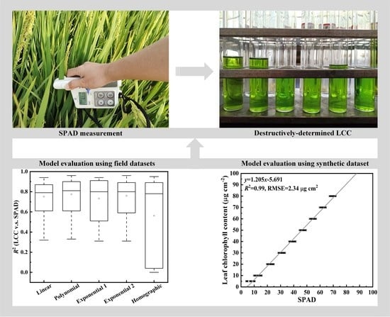
2. Materials and Methods

2.1. Datasets

2.1.1. Field Datasets

To study and assess the relationship between SPAD meter readings and LCC, we extracted three independent datasets published by Delegido et al. (2011) [8], Vuolo et al. (2012) [33], and Houborg et al. (2009) [34]. Hereafter, they are referred to as the Delegido’s, Vuolo’s, and Houborg’s datasets, respectively. All three datasets include LCC measured using a destructive method in the laboratory and output readings measured using a SPAD meter in the field. The LCC of Delegido’s dataset was measured by high-performance liquid chromatography (HPLC), and that of Houborg’s dataset was measured spectrophotometrically after extraction of chlorophyll with dimethyl sulfoxide (DMSO). Unlike Delegido’s and Houborg’s datasets, the LCC of Vuolo’s dataset was determined by the procedure described by De Michele et al. (2009) [35]. LCC in these datasets exhibits diverse ranges across various agricultural vegetation species (

Table 1. Statistics of leaf chlorophyll content in Delegido’s, Vuolo’s, and Houborg’s datasets. S.D. is the standard deviation, C.V. is the coefficient of variation, and n represents the number of observations.

Data Sources	Species	n	Minimum (μg cm−2)	Maximum (μg cm−2)	Mean (μg cm−2)	S.D. (μg cm−2)	C.V. (%)
Delegido et al. (2011)	Wheat	20	9.40	46.79	38.17	7.38	19.33
	Sugar beet	29	15.12	35.48	28.74	4.63	16.11
	Barley	20	23.10	54.88	35.46	9.05	25.53
	Corn	36	15.00	43.57	32.27	8.02	24.85
Vuolo et al. (2012)	Bean	32	1.86	43.26	25.54	11.68	46.00
	Grass	23	2.38	37.62	16.69	9.25	55.43
	Wheat	30	1.40	47.44	21.29	13.98	65.66
	Linseed	28	2.79	58.14	29.09	16.77	57.64
	Corn	28	3.26	34.42	16.73	10.36	61.94
	Oat	30	3.26	55.35	28.67	15.05	52.48
	Olive	26	9.30	58.14	30.25	11.95	39.49
	Orange	24	4.19	28.84	14.52	6.76	46.59
	Vine	25	9.77	28.84	18.40	6.07	32.96
Houborg et al. (2009)	Corn	48	12.20	86.34	50.82	18.92	37.23

).

Delegido’s dataset consists of LCC and SPAD values for four crops: wheat, sugar beet, barley, and corn. During field experiments, the selected samples considered discrepancies in LCC among individual leaves, single species, and different crop types. For each leaf sample, six measurements were made using a SPAD meter on selected parts of the leaf. Overall, the LCC of four crop species showed relative stability. The mean LCC of wheat was 38.17 μg cm⁻², with a minimum of 9.40 μg cm⁻² and a maximum of 46.79 μg cm⁻², and the LCC of sugar beet ranged between 15.12 μg cm⁻² and 35.48 μg cm⁻² with a mean value of 28.74 μg cm⁻². In comparison, the LCC of barley and corn had more substantial variation relative to wheat and sugar beet. The LCC of barley ranged from 23.10 μg cm⁻² to 54.88 μg cm⁻² with an average of 35.46 μg cm⁻², and that of corn varied from 15.00 μg cm⁻² to 43.57 μg cm⁻² with a mean value of 32.27 μg cm⁻². The four crops generally exhibited low-to-moderate LCC.

Vuolo’s dataset was collected in several field campaigns for nine agricultural species (i.e., bean, grass, wheat, linseed, maize, oat, olive, orange, and vine). Compared with Delegido’s dataset, the LCCs of these nine crops were more discrete and showed larger variation. In Vuolo’s dataset, the LCC of wheat changed most significantly among the nine species, varying between 1.40 μg cm⁻² to 47.44 μg cm⁻² with a mean value of 21.29 μg cm⁻² and C.V. of 65.66%. In contrast, the LCC of vine presented the smallest variation among these species, with a mean value of 18.40 μg cm⁻², a minimum of 9.77 μg cm⁻², and a maximum of 28.84 μg cm⁻². Similar to Delegido’s dataset, the LCC of the nine species ranged from low to medium.

Houborg’s dataset includes LCC and SPAD values for 48 corn samples. During field experiments, six measurements were conducted for each sample to properly characterize the variability of the LCC distribution across the leaves. LCC varied from 12.20 μg cm⁻² to 86.34 μg cm⁻², with a mean value of 50.82 μg cm⁻² and C.V. of 37.23%. The variation of LCC in Houborg’s dataset was between Delegido’s and Vuolo’s datasets. Moreover, Delegido’s, Vuolo’s, and Houborg’s datasets all possess the LCC of corn, whereas the variation of these three corn data is not fully identical. The LCC of corn in Vuolo’s dataset retained the most substantial variation, while that of Delegido’s dataset delivered the least variation among the three data. In addition, the LCC of corn in Delegido’s and Vuolo’s datasets ranged from low to moderate, while that in Houborg’s dataset exhibited a widely distributed LCC from low to high.

2.1.2. Simulated Dataset with the PROSPECT Model

In addition to the field datasets, we also generated a set of the simulated dataset using the PROSPECT model [36]. The PROSPECT model used in this study is PROSPECT-5, which is a physical model simulating leaf directional-hemispherical reflectance and transmittance using a suite of leaf biophysical and biochemical input parameters, namely leaf structure parameter (N), chlorophyll content ($C_{ab}$), carotenoid content ($C_{cx}$), brown pigments content ($C_{bp}$), equivalent water thickness ($C_w$), and dry matter content ($C_m$) [37]. A MATLAB version of the PROSPECT-5 model was downloaded from the following website: http://teledetection.ipgp.jussieu.fr/prosail/ (accessed on 17 May 2022). We obtained leaf transmittance spectra under various conditions by adjusting the input parameters and corresponding input values of the PROSPECT-5 model. In total, there were 2916 scenarios covering all the possible combinations in

Table 2. The input parameters and corresponding input values of the PROSPECT-5 model.

Parameter	Interpretation	Unit	Input Values
N	Leaf structure parameter	—	1.0, 2.0 or 3.0
$C_{ab}$	Chlorophyll a + b content	μg cm−2	5, 10, 20, 30, 40, 50, 60, 70 or 80
$C_{cx}$	Carotenoid content	μg cm−2	10, 20 or 30
$C_{bp}$	Brown pigments content	—	0.0, 0.5 or 1.0
$C_w$	Equivalent water thickness	cm	0.02, 0.04, 0.08 or 0.10
$C_m$	Dry matter content	g cm−2	0.005, 0.010 or 0.020

. The SPAD chlorophyll meter is developed based on spectral measurements of leaf transmittances at the wavelengths of 650 nm and 940 nm. Therefore, we converted the leaf transmittances generated for all synthetic scenarios into SPAD values according to the equation described by Raymond Hunt and Daughtry (2014) (i.e., Equation (1)). This equation can well express the relationship between the leaf transmittances and the SPAD values with a coefficient of determination (R²) of 0.998 across commonly used SPAD chlorophyll meters [38].

$$\mathrm{SPAD}=37\ast {\log }_{10}\left(\frac{T_{940}}{T_{650}}\right)-2.68$$

(1)

where SPAD is the SPAD value, and $T_{940}$ and $T_{650}$ are leaf transmittances at 940 nm and 650 nm, respectively.

2.2. Mathematical Functions for Relationships between SPAD Readings and LCC

We tested commonly used functional relationships between SPAD readings versus LCC in the literature, including linear, polynomial, exponential, and homographic functions. As shown in

Table 3. The commonly used functions for estimating leaf chlorophyll content (LCC in the unit of μg cm⁻²) from SPAD readings.

Model Forms	Equations	References
Linear	$\mathrm{LCC}=a\ast \mathrm{SPAD}+b$	Schaper and Chacko (1991)
Polynomial	$\mathrm{LCC}=a {\ast \mathrm{SPAD}}^2+b\ast \mathrm{SPAD}+c$	Monje and Bugbee (1992)
Exponential 1	$\mathrm{LCC}=a\ast e^{b\ast \mathrm{SPAD}}$	Uddling et al. (2007)
Exponential 2	$\mathrm{LCC}=0.0893\ast \left({10}^{{\mathrm{SPAD}}^{\alpha }}\right)$	Markwell et al. (1995)
Homographic	$\mathrm{LCC}=\frac{a \ast \mathrm{SPAD}}{b - \mathrm{SPAD}}$	Coste et al. (2010); Cerovic et al., (2012)

, the exponential functions have two different forms: one is $\mathrm{LCC}=a\ast e^{b\ast \mathrm{SPAD}}$ and the other is $\mathrm{LCC}=0.0893\ast \left({10}^{{\mathrm{SPAD}}^{\alpha }}\right)$. For the sake of distinction, they were named exponential 1 and exponential 2, respectively.

2.3. Accuracy Assessment

For the field datasets, the functional relationships between LCC and SPAD readings were evaluated for: (i) all datasets together, (ii) individual datasets from three different data sources, and (iii) individual vegetation species. For the synthetic dataset, we tested the relationships for different leaf structure parameters (i.e., N), each of which included 972 synthetic scenarios. We further investigated whether the choice of wavelengths could improve the relationships with LCC using 2916 scenarios of all possible combinations of the synthetic dataset in spite of differences in leaf structural parameters. To do this, we tested all possible combinations of wavelengths except those below 400 nm and above 1000 nm to check whether $T_{940}$ and $T_{650}$ are the best combinations for LCC estimation, since wavelengths outside this range were rarely used to estimate LCC and had large noise.

The coefficient of determination (R²) and root-mean-square error (RMSE) were registered as indicators of the strength of assessing each function. The R² is a measure of the degree of fitting between the independent and dependent variables, and the RMSE accounts for the difference between the estimated and observed values. The two metrics were used to comprehensively evaluate the accuracy of the functional relationships between LCC and SPAD values. The R² and RMSE can be calculated as follows:

$$R^2=1-\frac{{{\displaystyle \sum }}_{i=1}^n{\left({\widehat{y}}_i-y_i\right)}^2}{{{\displaystyle \sum }}_{i=1}^n{\left(y_i-\overline{y}\right)}^2}$$

(2)

$$\mathrm{RMSE}=\sqrt{\frac{1}{n}{\displaystyle \sum }_{i=1}^n{\left(y_i-{\widehat{y}}_i\right)}^2}$$

(3)

where $n$ is the number of observations, and $\overline{y}$ is the mean value of observations. ${\widehat{y}}_i$ and $y_i$ refer to the estimated and observed values for the i-th observation. The higher the R², the better the model fit, and the lower the RMSE, the closer the estimated value is to the observed value and the lower the estimated error.

3. Results

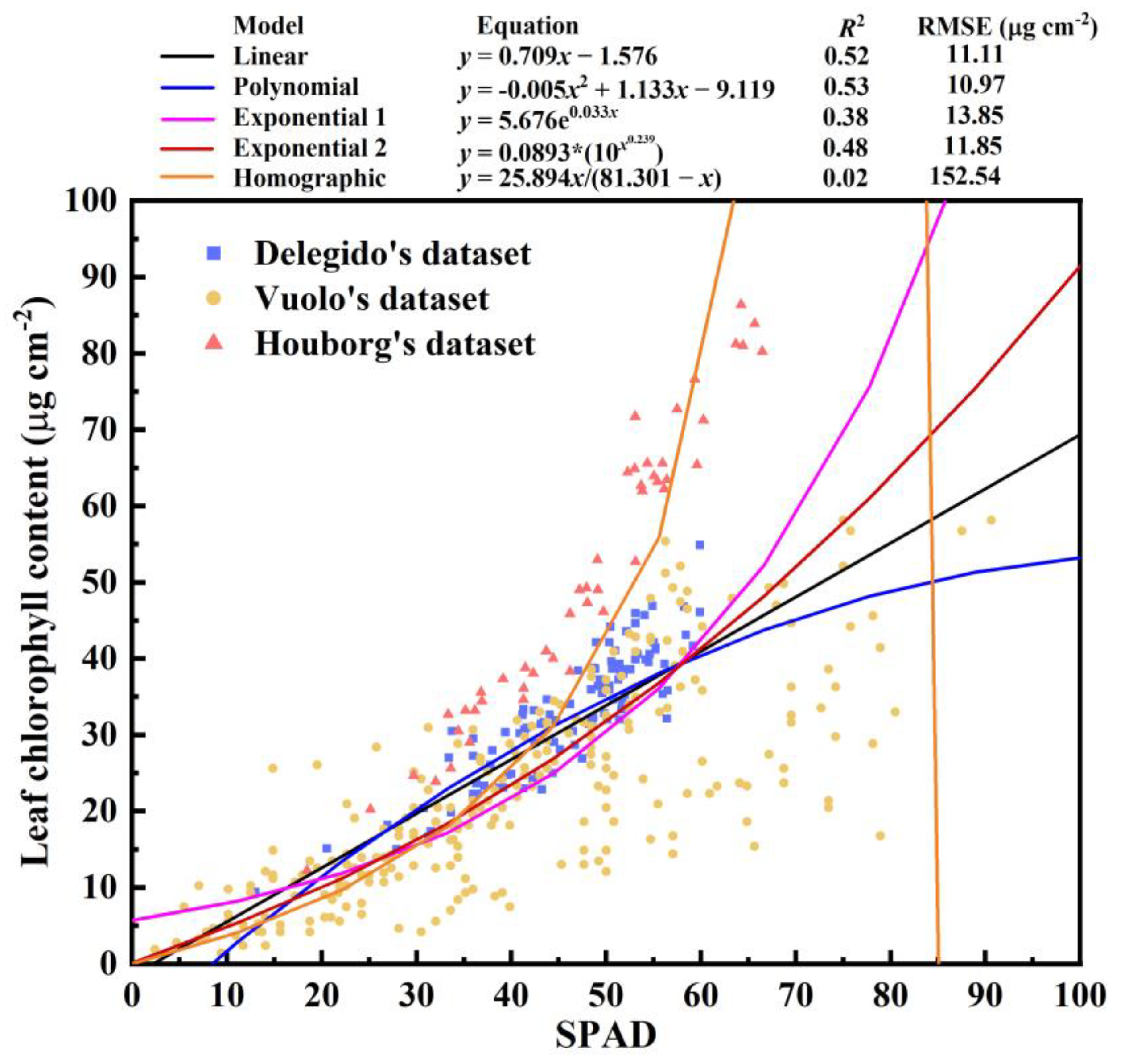
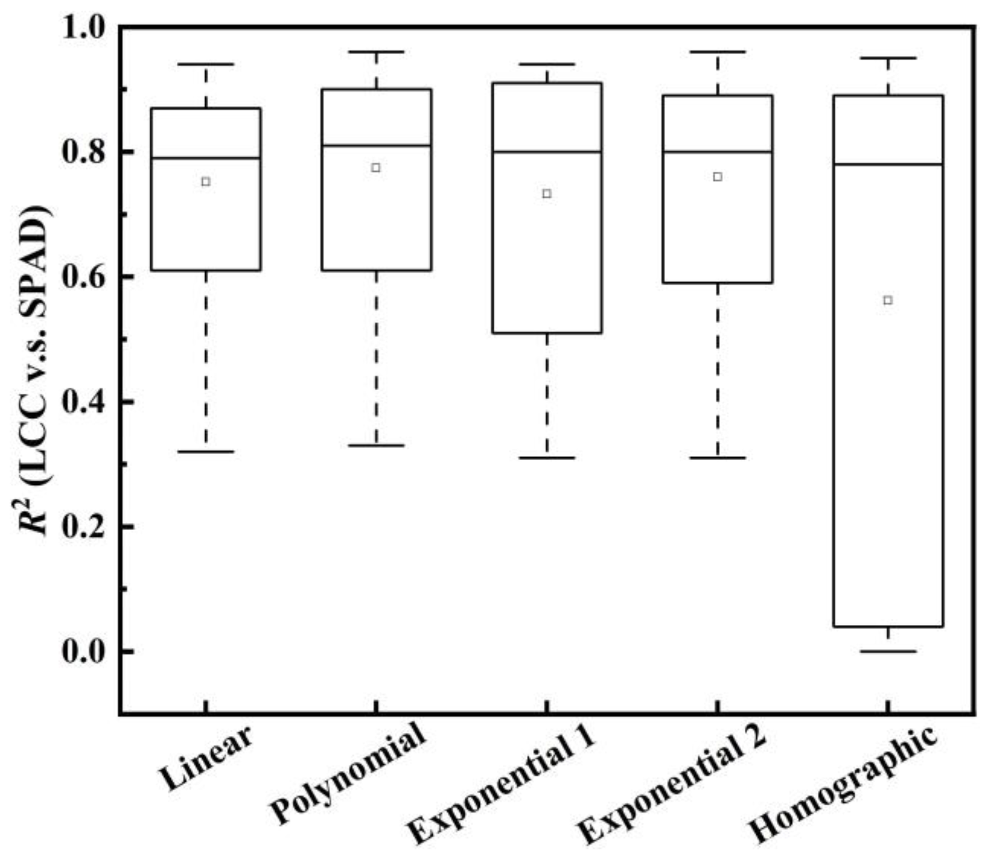
3.1. All the Field Datasets Together

We first established the linear, polynomial, exponential, and homographic functional relationships between LCC and SPAD readings for all three datasets together to evaluate their potential for estimating LCC without taking the differences in the datasets and species into consideration (Figure 1). The linear, polynomial, and exponential 2 ($\mathrm{LCC}=0.0893\ast \left({10}^{{\mathrm{SPAD}}^{\alpha }}\right))$ functional relationships between LCC and SPAD readings were promising with the R² as high as ~0.5, while the exponential 1 (i.e., $\mathrm{LCC}=a\ast e^{b\ast \mathrm{SPAD}}$) function performed slightly deficiently with an R² of 0.38, and the homographic function was the poorest with an R² of 0.02. The quadratic coefficient of the polynomial function was approximately zero, making it level off to the linear function. Therefore, regardless of the differences in the datasets and species, the linear, polynomial, and exponential functions were suited for estimating the LCC, whereas the homographic function was less suitable for the LCC estimation.

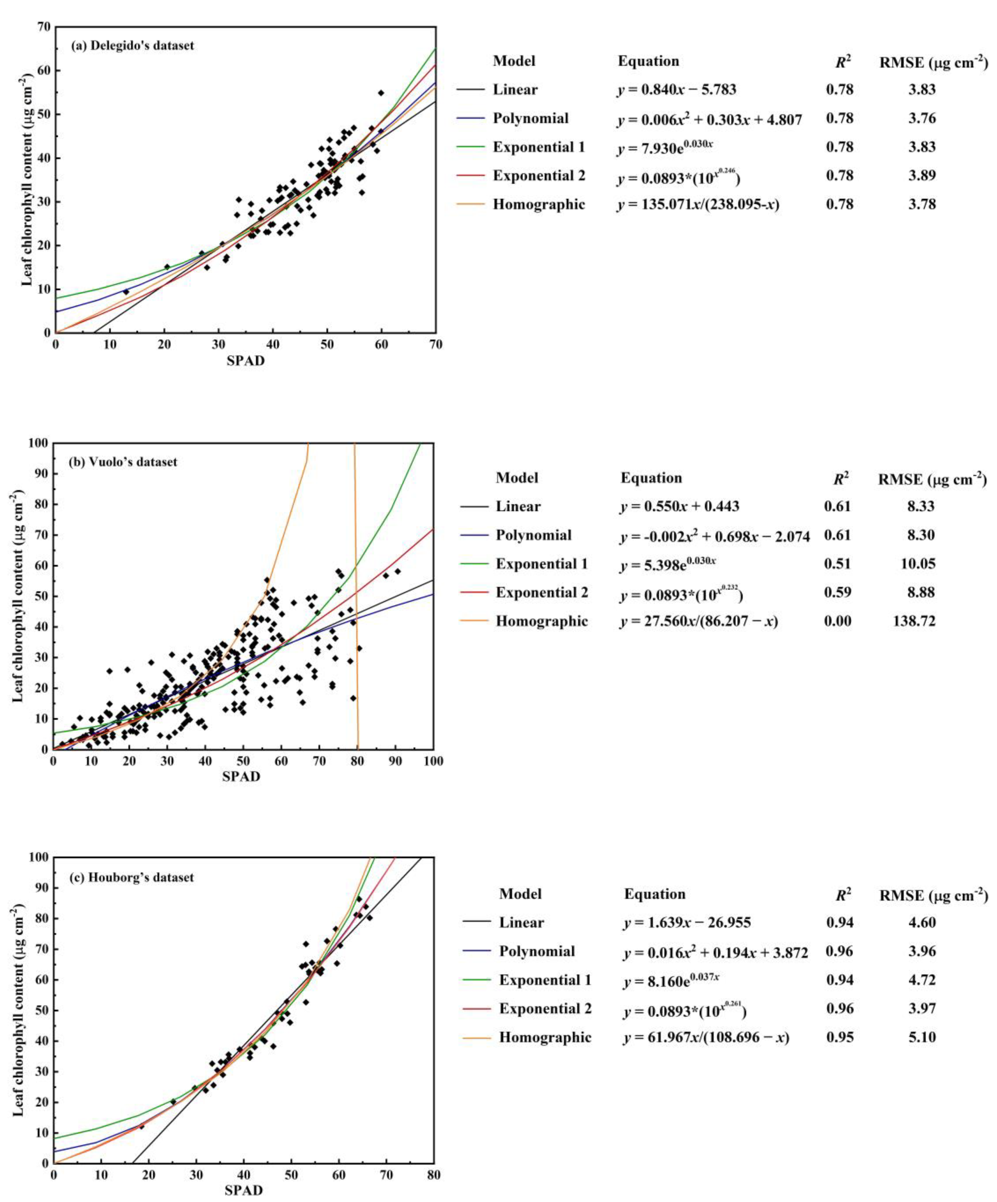
3.2. For Each Field Dataset

The linear, polynomial, exponential, and homographic functional relationships between LCC and SPAD readings were established for all species of each dataset to assess their performance in estimating the LCC (Figure 2). Compared with the performance of functional relationships across all three datasets together, the linkages between LCC and SPAD readings for the individual dataset were significantly improved. The five functions fitted comparably well the LCC and SPAD values for the four species in Delegido’s dataset with an R² of ~0.78, and their errors were small with an RMSE of ~3.82 μg cm⁻² (i.e., mean RMSE of the five functions). However, the homographic function was inferior to the other four functions for the nine species in Vuolo’s dataset with an R² of ~0.00 and RMSE of ~138.72 μg cm⁻². Especially at high SPAD values, similar to the results in Section 3.1, the homographic fitting curve shifted from monotonically increasing to sharply decreasing, even making the estimated LCC negative. Similar to Delegido’s dataset, the five SPAD–LCC functional relationships were comparable for the corn crop in Houborg’s dataset with an R² of ~0.95 and RMSE of ~4.47 μg cm⁻², whereas they generally excelled those expressed in Delegido’s dataset. In general, the linear, polynomial, and exponential functions could reasonably express associations between LCC and SPAD readings without considering differences in species, and the polynomial function could be approximated by the linear function because its quadratic coefficient was as small as zero. However, the exponential 1 function changed slightly, and the homographic function had significant variability across various vegetation species.

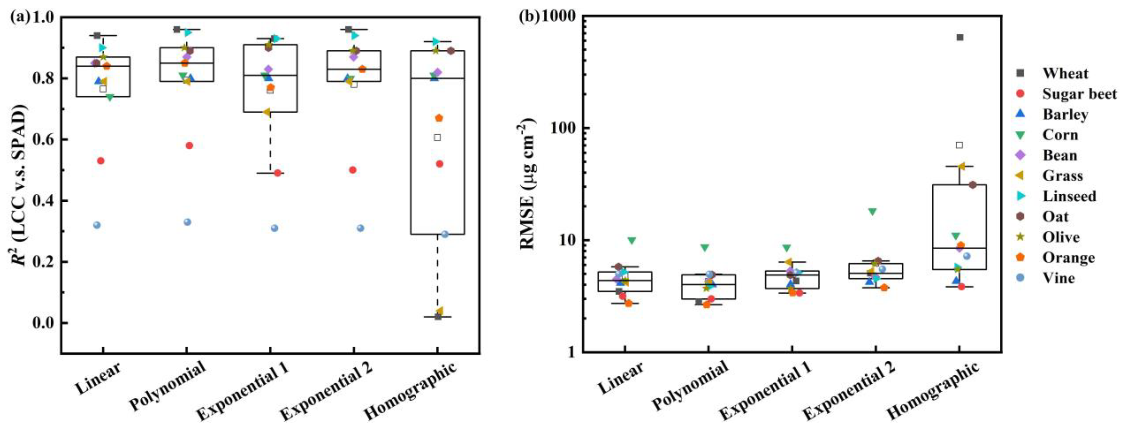
3.3. For Each Species

The linkages between the absolute measures of the LCC and the SPAD meter readings were recalibrated for the individual species within all the field datasets. The field datasets include absolute LCC and relative SPAD values for 11 species in total (i.e., wheat, sugar beet, barley, corn, bean, grass, linseed, oat, olive, orange, and vine). As with the model evaluations for the individual dataset in Section 3.2, the linear, polynomial, and exponential functional relationships between LCC and SPAD readings were satisfactory for most species (with an R² of not less than ~0.8 and RMSE less than 10 μg cm⁻²) (Figure 3). In comparison, the linear and polynomial functions were slightly better than the exponential functions. However, the performance of the homographic function exhibited substantial variation. In wheat and grass, it performed poorly with the R² of 0.02 and 0.04 and RMSE of up to 642.50 μg cm⁻² and 45.49 μg cm⁻², respectively. However, in other species, the homographic function had similar performance to the linear, polynomial, and exponential functions. Similar to the results in Section 3.2, linear, polynomial, and exponential 2 functions performed similarly promisingly. In contrast, the performance of the exponential 1 function varied little, and the homographic function changed significantly.

Combining the model evaluations of the above three aspects, we documented the distribution of R² and RMSE for the five functions in Figure 4. Similar to the results in Section 3.2 and Section 3.3, there was slight variability in the exponential 1 function, and the performance of the homographic function exhibited considerable variation and more caution was required when using this type of function for an unknown species. In comparison, the linear, polynomial, and exponential 2 functions were sufficiently accurate for most cases. Taking into account the fact that even though the variation range of α in the exponential 2 function is smaller than coefficients from other functions, small changes of α can lead to very large differences in LCC, such as corn in Figure 3b, and polynomial functions have quadratic coefficients close to zero according to the above results. Therefore, we recommended using a linear function to estimate LCC and listed the fitting coefficients of linear functions for specific vegetation species in

Table 4. Assessments of the linear function based on all datasets together, individual datasets, and each species per dataset in terms of three field datasets.

Data Sources	Species	a	b	R2	RMSE (μg cm−2)
All	All	0.709	−1.576	0.52	11.11
Delegido et al. (2011)	Wheat	0.788	−1.053	0.88	2.56
	Sugar beet	0.486	8.664	0.53	3.16
	Barley	1.174	−22.248	0.79	4.13
	Corn	0.879	−8.602	0.84	3.17
	All	0.840	−5.783	0.78	3.83
Vuolo et al. (2012)	Bean	0.770	−6.765	0.85	4.48
	Grass	0.797	−7.232	0.79	4.22
	Wheat	0.879	−9.350	0.94	3.28
	Linseed	0.776	−7.157	0.90	5.20
	Maize	0.664	−1.761	0.88	3.62
	Oat	0.828	−1.520	0.85	5.78
	Olive	0.875	−27.494	0.87	4.36
	Orange	0.388	−5.950	0.84	2.73
	Vine	0.495	4.376	0.32	5.00
	All	0.550	0.443	0.61	8.33
Houborg et al. (2009)	Corn/All	1.639	−26.955	0.94	4.60

for future usage.

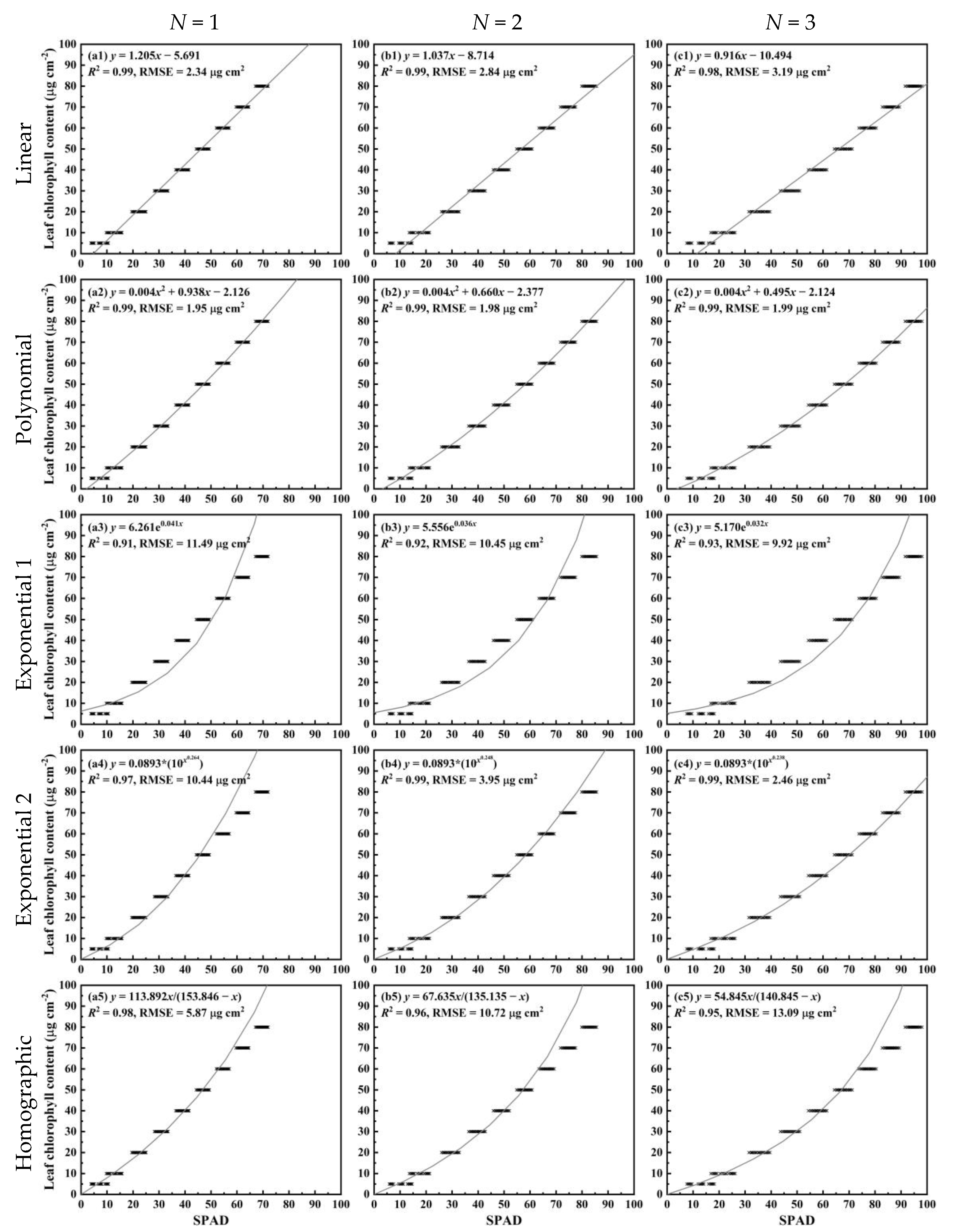
3.4. For the Simulated Dataset from the PROSPECT Model

In the simulated dataset, the linear, polynomial, exponential, and homographic functional relationships between LCC and SPAD values were established across various leaf structural parameters. For each type of leaf structure, a total of 972 LCC and SPAD values were fitted by five functions. Similar to the evaluation results of field datasets from three aspects, the linear, polynomial, and exponential 2 functions performed well with the R² of ~0.99 over different leaf structural parameters (Figure 5), while the estimation error of the exponential 2 function had a large variation from RMSE = 10.44 μg cm⁻² for N = 1 to RMSE = 2.46 μg cm⁻² for N = 3. In comparison, the exponential 1 function showed a slight change, and the homographic function varied significantly. The secondary coefficient of the polynomial function was approximately zero, making it close to the linear function, implying that when the leaf structure was determined, the SPAD reading had a significantly linear relationship with the LCC. Moreover, the performance of the linear, polynomial, and homographic functions decreased with increasing leaf structural parameters, whereas the behavior of the two exponential functions was reversed.

To test the relationship between different transmittance ratios and LCC and check whether $T_{940}$ and $T_{650}$ are the best combinations for LCC estimation, we further evaluated the relationships between the transmittance-based index (including ${\log }_{10}\left(T_{\lambda 1}/T_{\lambda 2}\right)$ and $T_{\lambda 1}/T_{\lambda 2}$) and LCC using all possible combinations of wavelengths. In the case of ${\log }_{10}\left(T_{\lambda 1}/T_{\lambda 2}\right)$, the transmittance-based index was strongly related with LCC provided that ${\lambda }_1$ was located in the near-infrared region (between 700 nm and 1000 nm) and ${\lambda }_2$ was located in the visible range (between 400 and 700 nm) and vice versa. The best combination of wavelengths was found in the red-edge region, especially when ${\lambda }_1=677\mathrm{nm}$ and ${\lambda }_2=679\mathrm{nm}$ (i.e., ${\log }_{10}\left(T_{677}/T_{679}\right)$), when the highest R² value achieved was as high as 1.00 (Figure 6a), providing some improvement over the SPAD meter (R² = 0.90 for ${\log }_{10}\left(T_{940}/T_{650}\right)$). Similar to ${\log }_{10}\left(T_{\lambda 1}/T_{\lambda 2}\right)$, the transmittance-based index $T_{\lambda 1}/T_{\lambda 2}$ had the highest R² at ${\lambda }_1=677\mathrm{nm}$ and ${\lambda }_2=679\mathrm{nm}$ (R² = 1.00) (Figure 6b), improving estimates of LCC over the SPAD meter. However, it had a generally lower relationship with LCC compared with ${\log }_{10}\left(T_{\lambda 1}/T_{\lambda 2}\right)$, which was in line with the logarithmic algorithm of the transmittance ratio designed by the SPAD meter. For the wavelengths used in the SPAD meter, the R² of the logarithm of the transmittance ratio (R² = 0.90 for ${\log }_{10}\left(T_{940}/T_{650}\right)$) was significantly higher than the simple transmittance ratio (R² = 0.50 for $T_{940}/T_{650}$).

4. Discussion

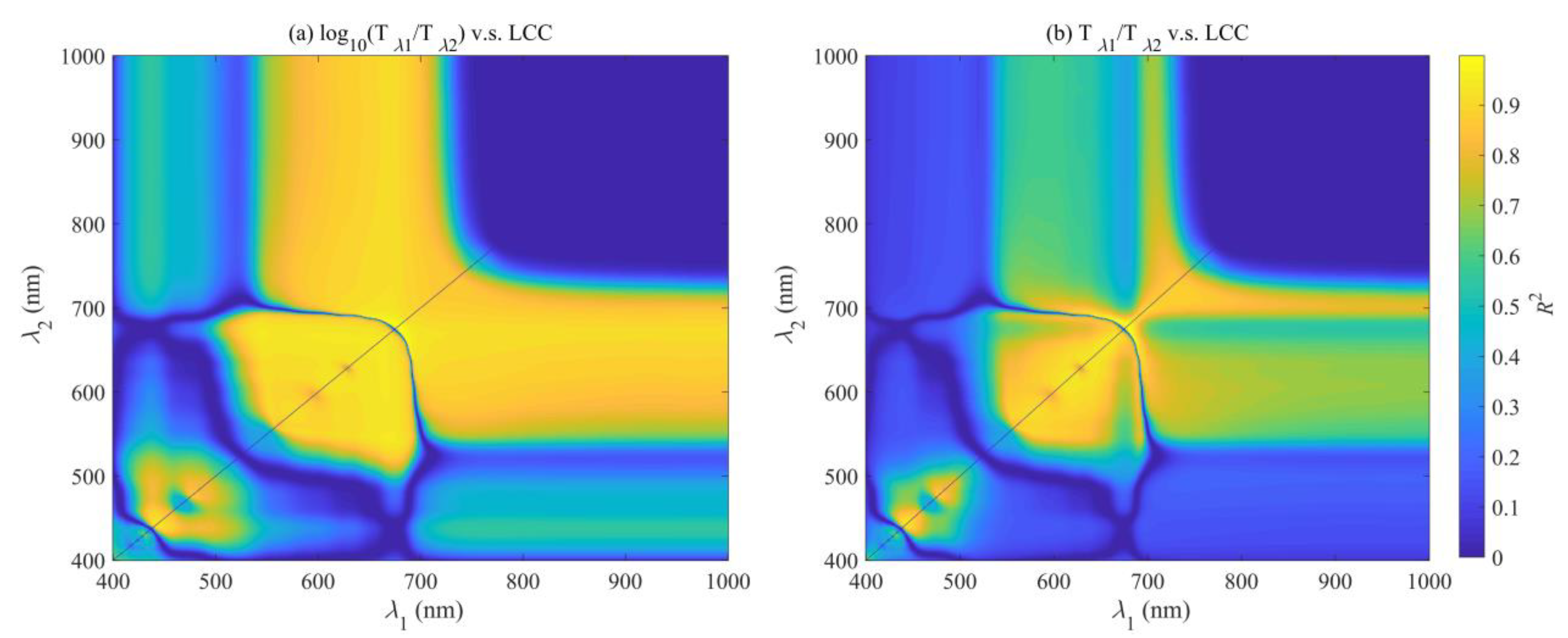
4.1. Relationship between LCC and SPAD Readings

The quantitative interpretation of the relationship between SPAD readings and LCC has been complicated by the fact that no algorithm is given in the SPAD manual to link meter output values with LCC. The relationship between LCC and SPAD readings is affected by multiple confounding factors such as leaf internal structure, leaf water content, and leaf pigment distribution [39,40,41]. Incident photons reaching the leaf surface are either absorbed, reflected, or transmitted, and their fates are significantly affected by the chlorophyll distribution inside the leaf. However, if we assume a leaf is a turbid medium and ignore the reflection in the air–leaf surface, the relationship between SPAD readings and the LCC of a leaf can be approximated by using Beer’s law. According to the designed algorithm of SPAD meters (Equation 1), the SPAD reading is proportional to the logarithm of the ratio of leaf transmittances at the wavelengths of 940 nm and 650 nm, i.e., $\mathrm{SPAD}\propto {\log }_{10}\left(T_{940}/T_{650}\right)$. In Beer’s law, the absorbance $A_{\lambda }$ and transmittance $T_{\lambda }$ of a leaf at a specific wavelength (λ) are related as $T_{\lambda }={10}^{-A_{\lambda }}$ [42]. Therefore, the SPAD value is proportional to the difference in leaf absorbances at 650 nm and 940 nm, which can be expressed as:

$$\mathrm{SPAD}\propto {\log }_{10}\left(\frac{T_{940}}{T_{650}}\right)={\log }_{10}\left(\frac{{10}^{-A_{940}}}{{10}^{-A_{650}}}\right)=A_{650}-A_{940}$$

(4)

The absorbance can be linked with the molar absorptivity $\epsilon$, content/concentration of the absorbing substance $C,$ and the length of the light path in the absorbing medium $b$, i.e., $A=\epsilon bC$. The absorbances at the wavelengths of 650 nm and 940 nm yield:

$$A_{650}=b\sum {\epsilon }_i^{650}{C}_i+b{\epsilon }_{chl}^{650}\mathrm{LCC}$$

(5)

$$A_{940}=b\sum {\epsilon }_i^{940}{C}_i+b{\epsilon }_{chl}^{940}\mathrm{LCC}$$

(6)

where $b$ is the length of the path that light travels in an absorbing medium, which is related to leaf structure. ${\epsilon }_i^{\lambda }$ and $C_i$ are the molar absorptivity at a specific wavelength and corresponding concentrations of other specific leaf constituents except for chlorophyll, respectively. ${\epsilon }_{chl}$ and $\mathrm{LCC}$ are the molar absorptivity of chlorophyll and leaf chlorophyll content, respectively.

Since chlorophyll has a strong absorption at 650 nm, and the absorbance at 940 nm is not sensitive to chlorophyll, it can be obtained that the absorption from chlorophyll at 940 nm (i.e., $b{\epsilon }_{chl}^{940}\mathrm{LCC}$) is negligible and the difference between the absorbances at 650 nm and 940 nm is:

$$A_{650}-A_{940}=b\sum \left({\epsilon }_i^{650}-{\epsilon }_i^{940}\right)C_i+b{\epsilon }_{chl}^{650}\mathrm{LCC}$$

(7)

The molar absorptivity $\epsilon$ is a constant for a specific constituent. Therefore, for leaves that vary only in LCC, SPAD readings should theoretically be linearly proportional to LCC: $\mathrm{SPAD}\propto b{\epsilon }_{chl}^{650}\mathrm{LCC}$. The simulations from the PROSPECT-5 model in Figure 5 confirm the linear relationship between SPAD readings and LCC when the length of the path traveled by light in the absorbing medium or leaf structure is constant. In most cases, even though the polynomial function is slightly better than the linear functions, its secondary coefficient is approaching zero, making it close to linear functions. Furthermore, in the small range of LCC, the exponential function can be approximated by the linear function.

However, in reality, the content/concentration of other constituents $C_i$ and the optical length $b$ usually vary among leaves due to the sieve effect and the detour effect caused by spatial heterogeneity of chlorophyll distribution within leaves. The so-called sieve effect occurs when light passes through leaf tissue without encountering an absorber, which leads to an increase in the transmittance, and thus the SPAD reading is lower than that of a leaf with uniform chlorophyll distribution [21,30]. The detour effect increases the optical path length through the leaf and reduces light transmission in the visible spectral region, resulting in higher SPAD readings compared to leaf samples with uniform chlorophyll distribution [43,44]. As a result, the linear relationship between SPAD readings and LCC is less reliable, and a universally applicable and analytical relationship is difficult to establish. Nonetheless, the linear functions are still promising for most cases, since LCC usually shows the largest variability compared with other leaf pigments. For different species, leaf structure can be different. In this case, one linear function for several species might not be sufficient (Figure 1). One solution to reduce the impact of leaf structure and other constituents on LCC estimation would be to establish one linear function for each species (Figure 3).

Alternatively, polynomial, exponential, and homographic functions are developed to account for the effects of variation in other leaf constituents and optical lengths. The increasing leaf structural parameters (i.e., N) may lead to the increased heterogeneity of chlorophyll distribution inside the leaf, which in turn results in the relationship between SPAD readings and LCC deviating more from linearity and enhancing the exponential functional relationship (Figure 5). As in the field datasets, the leaf cannot simply be treated as a turbid medium, and by extension, Beer’s law is not fully valid. Therefore, the different functions show different estimation accuracy in the field datasets.

In addition to the above ways of improving the estimates of LCC with the SPAD meter, a backup solution is to update/improve the algorithm designed by the SPAD meter using the optimal combination of wavelengths. The band combination ${\log }_{10}\left(T_{677}/T_{679}\right)$ based on the synthetic dataset provides the best relationship with LCC, significantly improving the estimation accuracy of LCC compared to the original algorithm designed by the SPAD meter (Figure 6). This is similar to the results presented by Brown et al. (2022), who reported that transmittance spectroscopy could provide improved performance over the SPAD meter using a range of field-measured datasets [45]. The fact that the optimal bands are related to wavelengths not measured by the SPAD meter suggests that it may not utilize all relevant spectral information, such as that contained at the red-edge wavelengths. Indeed, Gitelson et al. (2003) demonstrated that information from the red-edge region has previously been used to improve the estimation of LCC using reflectance-based indices [46]. Given the significant chlorophyll absorption characteristics in the red-edge region (around 680 nm) of the spectrum [47,48], the use of red-edge wavelengths has a clear physical basis.

4.2. Comparison of Different Functions

We evaluated the linear, polynomial, exponential, and homographic functional relationships between LCC and SPAD readings using three field datasets and one synthetic dataset. For the field datasets, we compared the performance of these five functions from three different aspects (i.e., all datasets together, individual datasets, and individual vegetation species). Model evaluations based on all datasets together showed that linear, polynomial, and exponential functions were able to reasonably estimate LCC, similar to the results revealed by Schaper and Chacko (1991), Monje and Bugbee (1992), and Uddling et al. (2007). In contrast, the homographic functions were less reliable for several cases, indicating this type of function is sensitive to the dataset and/or species. The nature of the leaves in the field datasets does not fulfill the turbid medium assumption underlying the designed algorithm of the SPAD meters. Hence, the linear relationship between LCC and SPAD readings was relatively weak for all field datasets since various vegetation types of leaves were examined together.

We further evaluated the performance of the five functions for estimating LCC for the single dataset and species of three field datasets. For a single species in the field datasets, the relationships between SPAD readings and LCC significantly improved compared to all datasets together. The result supports the hypothesis that differently distributed data sources decrease the association between LCC and SPAD readings. In most cases, the accuracy of the polynomial function is overall slightly higher than that of the linear function, partly due to the different variations in LCC and SPAD values for some species. However, the quadratic coefficient of the polynomial function is close to zero, causing it to approach a linear function, and it has higher degrees of freedom than the linear function, making it inappropriate when the amount of data for calibration is insufficient. Therefore, linear and exponential functions are recommended for a small amount of data, and polynomial functions are suitable for sufficient data. The homographic functions have significant variability, especially as the SPAD value approaches the calibration coefficient b, and numerical singularity will occur in this function since the denominator gradually approaches zero. All three field datasets include corn data, and the three corn data show different variations, perhaps because leaf samples of the corn collected in the three datasets were in diverse growth conditions. The different growth vigor may alter the relationship between LCC and SPAD readings in plant species, resulting in different functions for the same species in different datasets (Table 4). This is similar to the results delivered by Jiang et al. (2017), who demonstrated the mathematical model used to estimate LCC with SPAD readings is different for leaves at different growth stages [49]. The differences in growth conditions of vegetation species should be taken into account as much as possible when using SPAD meters to accurately estimate LCC.

As for the synthetic dataset, the linear functions perform better than other functions across various leaf structure parameters, probably because of the turbid medium assumption of the PROSPECT-5 leaf radiative transfer model. Synthesizing model evaluation results and analysis of the field and simulated datasets, we summarized the strengths and deficiencies of these five functions in

Table 5. Comparison of five functions for estimating the LCC with SPAD readings.

Models	Deficiencies
$\mathrm{LCC}=a\ast \mathrm{SPAD}+b$	Relatively lower accuracy compared to a polynomial model
$\mathrm{LCC}=a {\ast \mathrm{SPAD}}^2+b\ast \mathrm{SPAD}+c$	Unsuitable for limited data
$\mathrm{LCC}=a\ast e^{b\ast \mathrm{SPAD}}$	Moderate dependence on dataset and species Slightly lower accuracy than the linear and polynomial models
$\mathrm{LCC}=0.0893\ast \left({10}^{{\mathrm{SPAD}}^{\alpha }}\right)$	Slightly lower accuracy than the linear and polynomial models
$\mathrm{LCC}=\frac{a \ast \mathrm{SPAD}}{b - \mathrm{SPAD}}$	Strong dependence on dataset and species Significant variability Numerical singularity

to help select the appropriate function for absolute LCC estimation using SPAD meters in the field.

4.3. Limitations

We explored the potential of linear, polynomial, exponential, and homographic functions for LCC estimation using three field datasets and one synthetic dataset, but model evaluations based on field and simulated datasets also have several limitations. In the field datasets, the data we used are mostly agricultural vegetation types. Nevertheless, the study is still indicative and can be extended to forest leaves. The difference between agricultural species and forests is primarily reflected in the leaf structure, and the performance of estimating the LCC of forest leaves may be different for different functions. For example, the linear, polynomial, and homographic functions could effectively estimate the LCC of 13 neotropical trees with an R² of >0.80 [32], and the exponential function $\mathrm{LCC}=a\ast e^{b\ast \mathrm{SPAD}}$ showed promising results for the LCC estimation of six Amazonian tree species with an R² of 0.79 overall [50]. However, whether the exponential function $\mathrm{LCC}=0.0893\ast \left({10}^{{\mathrm{SPAD}}^{\alpha }}\right)$ is applicable to forest leaves and the variation of leaves in different woody types remains to be further investigated.

The model assessment from the synthetic dataset that we carried out is limited to the simple leaf radiative transfer model, PROSPECT-5. The synthetic dataset only covers the scenarios of homogenous leaves. In the PROSPECT-5 model, the leaves are treated as a turbid medium, which does not consider the spatial heterogeneity of chlorophyll distribution inside the leaves. Investigation of the radiative transfer model for more complex leaf conditions is required. Stuckens et al. (2009) have developed a dorsiventral leaf model (DLM) to simulate the radiative transfer of photons within the leaves by considering the influence of the leaf asymmetry caused by the non-uniform distribution of pigments, water, and dry matter, and by mimicking light scattering for adaxial and abaxial leaf surfaces [51]. In future studies, a specially designed experiment integrated with DLM or other similar models may lead to an improved understanding of the mechanical relationship between SPAD readings and LCC. Despite the limitations, the results presented in this study are similar to previous studies, and the use of simulated datasets and theoretical analysis can help to further understand the relationship between SPAD readings and LCC.

5. Conclusions

In this study, we used three field datasets from existing research and one synthetic dataset from the leaf transfer model PROSPECT-5 to assess the commonly used functions that convert SPAD readings into absolute LCC values. The linear function outperforms other functions in the simulated dataset, in which leaves show a relatively simple structure due to the assumption of a turbid medium in the PROSPECT-5 model. The linear relationship between SPAD readings and LCC revealed by the synthetic dataset is in line with the algorithm designed by the SPAD meter, which assumes leaf samples to be a turbid medium. Compared with the synthetic dataset, the leaves in the field datasets are more complex in terms of leaf structure and present more confounding factors. Thus, more complex functions (i.e., polynomial, exponential, and homographic functions) have been developed to link SPAD readings to LCC. We found that the functions do not work well for all three datasets together, while their performance is promising for a single dataset or species. The linear, polynomial, and exponential functions work similarly for various datasets and species with an R² of >0.8 and RMSE of <10 μg cm⁻² overall in the field datasets. In contrast, the homographic function has considerable dependence on datasets and species and is prone to numerical singularities due to the idiosyncrasies of the function per se. Therefore, more caution is needed when using this functional relationship to estimate LCC for an unknown species. The polynomial functions provide more freedom since one more fitting parameter is included, and they are approximated by linear models due to quadratic coefficients approaching zero. The study recommends the use of linear and exponential functions when calibration data for the conversion of SPAD readings into absolute LCC values are insufficient, and a polynomial function when the amount of calibration data is sufficient. The evaluation presented in this study is expected to assist in more accurately estimating absolute LCC using SPAD meters in the field.

References

1. Porcar-Castell, A.; Tyystjärvi, E.; Atherton, J.; Van Der Tol, C.; Flexas, J.; Pfündel, E.E.; Moreno, J.; Frankenberg, C.; Berry, J.A. Linking Chlorophyll a Fluorescence to Photosynthesis for Remote Sensing Applications: Mechanisms and Challenges. J. Exp. Bot. 2014, 65, 4065–4095. [Google Scholar] [CrossRef] [Green Version]
2. Croft, H.; Chen, J.M.; Luo, X.; Bartlett, P.; Chen, B.; Staebler, R.M. Leaf Chlorophyll Content as a Proxy for Leaf Photosynthetic Capacity. Glob. Chang. Biol. 2017, 23, 3513–3524. [Google Scholar] [CrossRef] [PubMed] [Green Version]
3. Palta, J.P. Leaf Chlorophyll Content. Remote Sens. Rev. 1990, 5, 207–213. [Google Scholar] [CrossRef]
4. Wang, S.; Li, Y.; Ju, W.; Chen, B.; Chen, J.; Croft, H.; Mickler, R.A.; Yang, F. Estimation of Leaf Photosynthetic Capacity from Leaf Chlorophyll Content and Leaf Age in a Subtropical Evergreen Coniferous Plantation. J. Geophys. Res. Biogeosciences 2020, 125, e2019JG005020. [Google Scholar] [CrossRef]
5. Zhang, J.; Blackmer, A.M.; Ellsworth, J.W.; Koehler, K.J. Sensitivity of Chlorophyll Meters for Diagnosing Nitrogen Deficiencies of Corn in Production Agriculture. Agron. J. 2008, 100, 543–550. [Google Scholar] [CrossRef]
6. Eitel, J.U.H.; Long, D.S.; Gessler, P.E.; Hunt, E.R. Combined Spectral Index to Improve Ground-Based Estimates of Nitrogen Status in Dryland Wheat. Agron. J. 2008, 100, 1694–1702. [Google Scholar] [CrossRef] [Green Version]
7. Lichtenthaler, H.K. Chlorophylls and Carotenoids: Pigments of Photosynthetic Biomembranes. Methods Enzymol. 1987, 148, 350–382. [Google Scholar] [CrossRef]
8. Delegido, J.; Vergara, C.; Verrelst, J.; Gandía, S.; Moreno, J. Remote Estimation of Crop Chlorophyll Content by Means of High-Spectral-Resolution Reflectance Techniques. Agron. J. 2011, 103, 1834–1842. [Google Scholar] [CrossRef]
9. Nishio, J.N. Why Are Higher Plants Green? Evolution of the Higher Plant Photosynthetic Pigment Complement. Plant Cell Environ. 2000, 23, 539–548. [Google Scholar] [CrossRef]
10. Sims, D.A.; Gamon, J.A. Relationships between Leaf Pigment Content and Spectral Reflectance across a Wide Range of Species, Leaf Structures and Developmental Stages. Remote Sens. Environ. 2002, 81, 337–354. [Google Scholar] [CrossRef]
11. Demmig-Adams, B.; Adams, W.W. The Role of Xanthophyll Cycle Carotenoids in the Protection of Photosynthesis. Trends Plant Sci. 1996, 1, 21–26. [Google Scholar] [CrossRef]
12. Barker, D.H.; Seaton, G.G.R.; Robinson, S.A. Internal and External Photoprotection in Developing Leaves of the CAM Plant Cotyledon Orbiculata. Plant Cell Environ. 1997, 20, 617–624. [Google Scholar] [CrossRef]
13. Castelli, F.; Contillo, R.; Miceli, F. Non-Destructive Determination of Leaf Chlorophyll Content in Four Crop Species. J. Agron. Crop Sci. 1996, 177, 275–283. [Google Scholar] [CrossRef]
14. Dong, T.; Shang, J.; Chen, J.M.; Liu, J.; Qian, B.; Ma, B.; Morrison, M.J.; Zhang, C.; Liu, Y.; Shi, Y.; et al. Assessment of Portable Chlorophyll Meters for Measuring Crop Leaf Chlorophyll Concentration. Remote Sens. 2019, 11, 2706. [Google Scholar] [CrossRef] [Green Version]
15. Lichtenthaler, H.K.; Wellburn, A.R. Determinations of Total Carotenoids and Chlorophylls a and b of Leaf Extracts in Different Solvents. Biochem. Soc. Trans. 1983, 11, 591–592. [Google Scholar] [CrossRef] [Green Version]
16. Shoaf, W.T.; Lium, B.W. Improved Extraction of Chlorophyll a and b from Algae Using Dimethyl Sulfoxide. Limnol. Oceanogr. 1976, 21, 926–928. [Google Scholar] [CrossRef]
17. Barnes, J.D.; Balaguer, L.; Manrique, E.; Elvira, S.; Davison, A.W. A Reappraisal of the Use of DMSO for the Extraction and Determination of Chlorophylls a and b in Lichens and Higher Plants. Environ. Exp. Bot. 1992, 32, 85–100. [Google Scholar] [CrossRef]
18. Shinano, T.; Lei, T.T.; Kawamukai, T.; Inoue, M.T.; Koike, T.; Tadano, T. Dimethylsulfoxide Method for the Extraction of Chlorophylls a and b from the Leaves of Wheat, Field Bean, Dwarf Bamboo, and Oak. Photosynthetica 1996, 32, 409–415. [Google Scholar]
19. Dugo, P.; Cacciola, F.; Kumm, T.; Dugo, G.; Mondello, L. Comprehensive Multidimensional Liquid Chromatography: Theory and Applications. J. Chromatogr. A 2008, 1184, 353–368. [Google Scholar] [CrossRef]
20. Ritchie, R.J. Consistent Sets of Spectrophotometric Chlorophyll Equations for Acetone, Methanol and Ethanol Solvents. Photosynth. Res. 2006, 89, 27–41. [Google Scholar] [CrossRef]
21. Richardson, A.D.; Duigan, S.P.; Berlyn, G.P. An Evaluation of Noninvasive Methods to Estimate Foliar Chlorophyll Content. New Phytol. 2002, 153, 185–194. [Google Scholar] [CrossRef]
22. Cerovic, Z.G.; Masdoumier, G.; Ghozlen, N.B.; Latouche, G. A New Optical Leaf-Clip Meter for Simultaneous Non-Destructive Assessment of Leaf Chlorophyll and Epidermal Flavonoids. Physiol. Plant. 2012, 146, 251–260. [Google Scholar] [CrossRef] [PubMed]
23. Hawkins, T.S.; Gardiner, E.S.; Comer, G.S. Modeling the Relationship between Extractable Chlorophyll and SPAD-502 Readings for Endangered Plant Species Research. J. Nat. Conserv. 2009, 17, 123–127. [Google Scholar] [CrossRef]
24. Shibaeva, T.G.; Mamaev, A.V.; Sherudilo, E.G. Evaluation of a SPAD-502 Plus Chlorophyll Meter to Estimate Chlorophyll Content in Leaves with Interveinal Chlorosis. Russ. J. Plant Physiol. 2020, 67, 690–696. [Google Scholar] [CrossRef]
25. Steele, M.R.; Gitelson, A.A.; Rundquist, D.C. A Comparison of Two Techniques for Nondestructive Measurement of Chlorophyll Content in Grapevine Leaves. Agron. J. 2008, 100, 779–782. [Google Scholar] [CrossRef] [Green Version]
26. Casa, R.; Castaldi, F.; Pascucci, S.; Pignatti, S. Chlorophyll Estimation in Field Crops: An Assessment of Handheld Leaf Meters and Spectral Reflectance Measurements. J. Agric. Sci. 2015, 153, 876–890. [Google Scholar] [CrossRef]
27. Botha, E.J.; Leblon, B.; Zebarth, B.J.; Watmough, J. Non-Destructive Estimation of Wheat Leaf Chlorophyll Content from Hyperspectral Measurements through Analytical Model Inversion. Int. J. Remote Sens. 2010, 31, 1679–1697. [Google Scholar] [CrossRef]
28. Schaper, H.; Chacko, E.K. Relation between Extractable Chlorophyll and Portable Chlorophyll Meter Readings in Leaves of Eight Tropical and Subtropical Fruit-Tree Species. J. Plant Physiol. 1991, 138, 674–677. [Google Scholar] [CrossRef]
29. Monje, O.A.; Bugbee, B. Inherent Limitations of Nondestructive Chlorophyll Meters: A Comparison of Two Types of Meters. HortScience 1992, 27, 69–71. [Google Scholar] [CrossRef] [Green Version]
30. Uddling, J.; Gelang-Alfredsson, J.; Piikki, K.; Pleijel, H. Evaluating the Relationship between Leaf Chlorophyll Concentration and SPAD-502 Chlorophyll Meter Readings. Photosynth. Res. 2007, 91, 37–46. [Google Scholar] [CrossRef]
31. Markwell, J.; Osterman, J.C.; Mitchell, J.L. Calibration of the Minolta SPAD-502 Leaf Chlorophyll Meter. Photosynth. Res. 1995, 46, 467–472. [Google Scholar] [CrossRef] [PubMed]
32. Coste, S.; Baraloto, C.; Leroy, C.; Marcon, É.; Renaud, A.; Richardson, A.D.; Roggy, J.-C.; Schimann, H.; Uddling, J.; Hérault, B. Assessing Foliar Chlorophyll Contents with the SPAD-502 Chlorophyll Meter: A Calibration Test with Thirteen Tree Species of Tropical Rainforest in French Guiana. Ann. For. Sci. 2010, 67, 607. [Google Scholar] [CrossRef] [Green Version]
33. Vuolo, F.; Dash, J.; Curran, P.J.; Lajas, D.; Kwiatkowska, E. Methodologies and Uncertainties in the Use of the Terrestrial Chlorophyll Index for the Sentinel-3 Mission. Remote Sens. 2012, 4, 1112–1133. [Google Scholar] [CrossRef] [Green Version]
34. Houborg, R.; Anderson, M.; Daughtry, C. Utility of an Image-Based Canopy Reflectance Modeling Tool for Remote Estimation of LAI and Leaf Chlorophyll Content at the Field Scale. Remote Sens. Environ. 2009, 113, 259–274. [Google Scholar] [CrossRef]
35. De Michele, C.; Vuolo, F.; D’Urso, G.; Marotta, L.; Richter, K. The Irrigation Advisory Program of Campania Region: From Research to Operational Support for the Water Directive in Agriculture. In Proceedings of the 33rd International Symposium on Remote Sensing of Environment, Stresa, Italy, 4–8 May 2009; Volume II, pp. 965–968. [Google Scholar]
36. Jacquemoud, S.; Baret, F. PROSPECT: A Model of Leaf Optical Properties Spectra. Remote Sens. Environ. 1990, 34, 75–91. [Google Scholar] [CrossRef]
37. Feret, J.-B.; François, C.; Asner, G.P.; Gitelson, A.A.; Martin, R.E.; Bidel, L.P.R.; Ustin, S.L.; le Maire, G.; Jacquemoud, S. PROSPECT-4 and 5: Advances in the Leaf Optical Properties Model Separating Photosynthetic Pigments. Remote Sens. Environ. 2008, 112, 3030–3043. [Google Scholar] [CrossRef]
38. Raymond Hunt, E.; Daughtry, C.S.T. Chlorophyll Meter Calibrations for Chlorophyll Content Using Measured and Simulated Leaf Transmittances. Agron. J. 2014, 106, 931–939. [Google Scholar] [CrossRef] [Green Version]
39. Padilla, F.M.; Gallardo, M.; Peña-Fleitas, M.T.; De Souza, R.; Thompson, R.B. Proximal Optical Sensors for Nitrogen Management of Vegetable Crops: A Review. Sensors 2018, 18, 2083. [Google Scholar] [CrossRef] [Green Version]
40. Fukshansky, L.; Remisowsky, A.M.V.; McClendon, J.; Ritterbusch, A.; Richter, T.; Mohr, H. Absorption Spectra of Leaves Corrected for Scattering and Distributional Error: A Radiative Transfer and Absorption Statistics Treatment. Photochem. Photobiol. 1993, 57, 538–555. [Google Scholar] [CrossRef]
41. Manetas, Y.; Grammatikopoulos, G.; Kyparissis, A. The Use of the Portable, Non-Destructive, SPAD-502 (Minolta) Chlorophyll Meter with Leaves of Varying Trichome Density and Anthocyanin Content. J. Plant Physiol. 1998, 153, 513–516. [Google Scholar] [CrossRef]
42. Swinehart, D.F. The Beer-Lambert Law. J. Chem. Educ. 1962, 39, 333. [Google Scholar] [CrossRef]
43. Parry, C.; Blonquist, J.M.; Bugbee, B. In Situ Measurement of Leaf Chlorophyll Concentration: Analysis of the Optical/Absolute Relationship. Plant Cell Environ. 2014, 37, 2508–2520. [Google Scholar] [CrossRef] [PubMed]
44. Nauš, J.; Prokopová, J.; Řebíček, J.; Špundová, M. SPAD Chlorophyll Meter Reading Can Be Pronouncedly Affected by Chloroplast Movement. Photosynth. Res. 2010, 105, 265–271. [Google Scholar] [CrossRef] [PubMed]
45. Brown, L.A.; Williams, O.; Dash, J. Calibration and Characterisation of Four Chlorophyll Meters and Transmittance Spectroscopy for Non-Destructive Estimation of Forest Leaf Chlorophyll Concentration. Agric. For. Meteorol. 2022, 323, 109059. [Google Scholar] [CrossRef]
46. Gitelson, A.A.; Gritz, Y.; Merzlyak, M.N. Relationships between Leaf Chlorophyll Content and Spectral Reflectance and Algorithms for Non-Destructive Chlorophyll Assessment in Higher Plant Leaves. J. Plant Physiol. 2003, 160, 271–282. [Google Scholar] [CrossRef]
47. Ustin, S.L.; Gitelson, A.A.; Jacquemoud, S.; Schaepman, M.; Asner, G.P.; Gamon, J.A.; Zarco-Tejada, P. Retrieval of Foliar Information about Plant Pigment Systems from High Resolution Spectroscopy. Remote Sens. Environ. 2009, 113, S67–S77. [Google Scholar] [CrossRef] [Green Version]
48. Clevers, J.G.P.W.; De Jong, S.M.; Epema, G.F.; Van Der Meer, F.; Bakker, W.H.; Skidmore, A.K.; Addink, E.A. MERIS and the Red-Edge Position. Int. J. Appl. Earth Obs. Geoinf. 2001, 3, 313–320. [Google Scholar] [CrossRef]
49. Jiang, C.; Johkan, M.; Hohjo, M.; Tsukagoshi, S.; Maruo, T. A Correlation Analysis on Chlorophyll Content and SPAD Value in Tomato Leaves. HortResearch 2017, 71, 37–42. [Google Scholar] [CrossRef]
50. Marenco, R.A.; Antezana-Vera, S.A.; Nascimento, H.C.S. Relationship between Specific Leaf Area, Leaf Thickness, Leaf Water Content and SPAD-502 Readings in Six Amazonian Tree Species. Photosynthetica 2009, 47, 184–190. [Google Scholar] [CrossRef]
51. Stuckens, J.; Verstraeten, W.W.; Delalieux, S.; Swennen, R.; Coppin, P. A Dorsiventral Leaf Radiative Transfer Model: Development, Validation and Improved Model Inversion Techniques. Remote Sens. Environ. 2009, 113, 2560–2573. [Google Scholar] [CrossRef]
Figure 1. The assessment of five functions (i.e., linear, polynomial, exponential 1, exponential 2, and homographic models) for the estimation of the LCC using all three field datasets together. Blue squares, pale-yellow dots, and red triangles represent Delegido’s, Vuolo’s, and Houborg’s datasets, respectively. Exponential 1 is the exponential function LCC = a e b SPAD , and Exponential 2 is the exponential function LCC = 0.0893 10 SPAD α . Note that the part of the homographic fitting curve is not shown because its value goes from incremental to negative infinity as the denominator of the function progressively approaches zero.
Remotesensing 14 05144 g001
Figure 2. The assessments of five functions for the estimation of the LCC of all species in Delegido’s (a), Vuolo’s (b), and Houborg’s dataset (c). The right panel corresponds to the statistics of the five function evaluations for each dataset in the left panel.
Remotesensing 14 05144 g002
Figure 3. The assessments of five functions for the estimation of the LCC of each species across all field datasets with the R2 (a) and RMSE (b). Exponential 1 is the exponential function LCC = a e b SPAD , and Exponential 2 is the exponential function LCC = 0.0893 10 SPAD α . Central lines represent the medians, boxes represent 50% of the data, squares represent mean values, whiskers represent minimum and maximum values, and symbols outside the whiskers represent outliers.
Remotesensing 14 05144 g003
Figure 4. Boxplots for the coefficients of determination of five functions for the relationships between LCC and SPAD readings based on the model assessments of field datasets from three aspects: (i) all datasets together, (ii) individual datasets from three different data sources, and (iii) individual vegetation species. Central lines represent the medians, boxes represent 50% of the data, squares represent mean values, and whiskers represent minimum and maximum values.
Remotesensing 14 05144 g004
Figure 5. The evaluations of five functions for estimating the LCC based on the simulated dataset from the PROSPECT-5 model. The left, middle, and right panels represent model evaluations for N = 1, N = 2, and N = 3, respectively. Exponential 1 is the exponential function LCC = a e b SPAD , and Exponential 2 is the exponential function LCC = 0.0893 10 SPAD α . N is the leaf structure parameter.
Remotesensing 14 05144 g005
Figure 6. Variation in R2 of relationships between the transmittance-based index and LCC, as a function of incorporated wavelengths, for log 10 T λ 1 / T λ 2 (a), and T λ 1 / T λ 2 (b).
Remotesensing 14 05144 g006