Article

Nonlinear Unmixing via Deep Autoencoder Networks for Generalized Bilinear Model

1
School of Artificial Intelligence, Xidian University, Xi’an 710071, China
2
School of Mathematics and Statistics, Xidian University, Xi’an 710071, China
*
Author to whom correspondence should be addressed.
Remote Sens. 2022, 14(20), 5167; https://doi.org/10.3390/rs14205167
Submission received: 29 August 2022 / Revised: 27 September 2022 / Accepted: 12 October 2022 / Published: 15 October 2022
(This article belongs to the Special Issue Deep Learning for the Analysis of Multi-/Hyperspectral Images)

Abstract

:
Hyperspectral unmixing decomposes the observed mixed spectra into a collection of constituent pure material signatures and the associated fractional abundances. Because of the universal modeling ability of neural networks, deep learning (DL) techniques are gaining prominence in solving hyperspectral analysis tasks. The autoencoder (AE) network has been extensively investigated in linear blind source unmixing. However, the linear mixing model (LMM) may fail to provide good unmixing performance when the nonlinear mixing effects are nonnegligible in complex scenarios. Considering the limitations of LMM, we propose an unsupervised nonlinear spectral unmixing method, based on autoencoder architecture. Firstly, a deep neural network is employed as the encoder to extract the low-dimension feature of the mixed pixel. Then, the generalized bilinear model (GBM) is used to design the decoder, which has a linear mixing part and a nonlinear mixing one. The coefficient of the bilinear mixing part can be adjusted by a set of learnable parameters, which makes the method perform well on both nonlinear and linear data. Finally, some regular terms are imposed on the loss function and an alternating update strategy is utilized to train the network. Experimental results on synthetic and real datasets verify the effectiveness of the proposed model and show very competitive performance compared with several existing algorithms.

1. Introduction

Hyperspectral images (HSIs), containing spatial and spectral information, are generated by imaging spectrometers mounted on various space platforms [1]. With the development of hyperspectral imaging technology, modern hyperspectral sensors can obtain hundreds of continuous spectral bands and reach nanometer-level spectral resolution [2,3]. The hyperspectral image is widely used in the areas of target detection and recognition, forest mapping, mineral exploitation, and other applications, due to its high spectral resolution. However, due to the limited spatial resolution of HSIs, several materials may appear simultaneously in the area covered by a single pixel, known as ‘‘mixed pixel’’ [1,4]. Mixed pixels have a significant impact on hyperspectral classification [5,6,7,8], target detection [9,10,11], and matching [12,13,14]. Therefore, hyperspectral unmixing (HU) is a hot research topic, which aims to address the decomposition problem of “mixed pixels” in hyperspectral images [15].
Hyperspectral data usually assumes that the spectrum of each pixel is a combination of a set of pure materials called endmembers and the corresponding proportion of each endmember, called abundances [16]. The purpose of HU is to estimate the endmember spectral signatures and the value of fractional abundances [3]. The mixture model associated with HU can be linear or nonlinear, depending on the hyperspectral image under study. Due to simplicity and physical interpretability, the linear mixing model (LMM) is the most widely used model in HU. LMM assumes that each observed pixel is a linear combination of endmember spectral signatures [17,18]. For the linear spectral unmixing, numerous classical algorithms have been proposed, such as minimum volume constrained nonnegative matrix factorization (MVCNMF) [19], vertex component analysis (VCA) [20], variable splitting and augmented Lagrangian sparse unmixing (SUnSAL) [21,22], and fully constrained least squares (FCLS) [23].
Although the linear mixing model (LMM) has shown excellent properties for macroscopic mixtures, LMM may lose its applicability in some natural scenes where there are small scale distributions of ground targets, large topographical fluctuations, and intimate mixing of specific materials. In response to the intractability of the nonlinear mixing effects, many nonlinear mixing models (NMM) have been developed. The kernel-based method is commonly used in nonlinear unmixing tasks. In [24,25], the radial basis kernel function is used to realize the unmixing of nonlinear mixed pixels. With the help of this technique, nonlinear data can be mapped onto a high-dimensional space where the relationship between the data can be stated linearly. In addition, some nonlinear unmixing methods are based on physical mixture models, such as the Hapke model [26,27] and geometric optics model [28]. The Hapke model, a mixing model based on specific ground materials, is the most prevalent and significant nonlinear model. However, the Hapke model needs lots of prior knowledge of ground materials, which limits its effective applications in practice. To simplify the nonlinear mixture effects, the bilinear mixing model (BMM) only considers the second-order scattering of the spectrum, and ignores the effect of high-order scattering [29]. The classic BMMs include the Nascimento model (NM) [30], the Fan model (FM) [31], and the generalized bilinear mixing model (GBM) [32]. The NM considers the second-order interactions between various endmembers, and the bilinear interaction terms can be regarded as extra endmembers. The FM assumes that the magnitude of the second-order products is related only to the abundances. In [32], the GBM, a generalization of the LMM and FM, was proposed, and different algorithms were studied to estimate the parameters of this bilinear model. Thereafter, different improved methods have been proposed for the GBM unmixing of hyperspectral images. Halimi et al. proposed a constrained projection optimal gradient method [33] and Yokoya et al. adopted semi-nonnegative matrix factorization as an optimization method for the GBM unmixing [34].
With the advent of deep learning, learning-based methods have many applications in hyperspectral unmixing. In [35], the nonlinear mixture model based on support vector machines and neural network-based techniques was used to estimate the fraction of abundances. In [36], the authors implemented a model-free unmixing method based on an auto-associative neural network to realize the mapping from the input pixel to the abundance percentages. In [37], the authors designed an end-to-end network for unmixing, and the convolutional neural network was used for extracting spatial information to improve the accuracy of unmixing. However, these methods require known ground truth abundance that is usually generated by other time-consuming labeling methods. The quality of the ground truth label drastically influences the performance of unmixing.
To overcome the limitation of supervised methods, unsupervised blind unmixing methods based on an autoencoder network have developed rapidly. An autoencoder consists of the encoder and the decoder. The encoder can map the input to low-dimensional embedding, and the decoder tries to restore the original input from low-dimensional embedding. Generally, since abundances can be considered as a low-dimensional representation of hyperspectral data, autoencoder networks are ideal for spectral unmixing. In [38], a stacked autoencoder and a variational autoencoder were implemented for unmixing. The stacked autoencoder, which can mitigate the effects of outliers, extracted endmember spectral signatures to generate a good initialization for the variational autoencoder. In [39], Palsson et al. used a full convolutional autoencoder to extract spatial features of pixels in a hyperspectral image, to estimate endmembers and abundance. In [40], the authors combined a shallow autoencoder with generative adversarial network (GAN) for spectral unmixing, and GAN was employed to improve the quality of reconstructed pixels. However, these methods were all used to solve the linear unmixing problem. Few researchers have focused on the application of autoencoder networks for nonlinear unmixing. In [41], the authors regarded hyperspectral data as a combination of the linear mixing part and nonlinear fluctuations. A pre-training technique was utilized to realize the mapping of nonlinear fluctuations. However, it was not convincing to use the same pixels as input and output in the process of pretraining to achieve a mapping of nonlinear fluctuations. Moreover, most papers consider the nonlinear model as the addition of the linear part and the nonlinear part. In [42], two deep autoencoders were employed to model the linear mixture and the second-order scattering interactions, respectively. In addition, the multi-task learning strategy was used to optimize two autoencoders jointly. In [43], the authors imposed a specific component on both the encoder and decoder, and considered the mixing model as a nonlinear fluctuation over a linear mixture. The nonlinear part of these models is learned by neural networks. In our paper, we seek a reconstruction network that integrates a linear part and a nonlinear one. Considering the simplicity and effectiveness of the GBM, we propose a blind source unmixing model based on a specially designed autoencoder network (GBM_AE), which divides the decoder into the linear decoder and the nonlinear one based on the GBM, and utilizes a deep encoder to extract features. The amplitude of the nonlinear mixing part is obtained by network feedforward. The main parts of the work are as follows:
  • Inspired by the widely used autoencoder network, we design a new deep autoencoder network structure based on the GBM, to achieve nonlinear unmixing. The deep encoder of the autoencoder is utilized to extract features. In the decoder part, the GBM is used to divide the decoder into a linear part and a nonlinear part. For the linear part of the decoder, we design a specific network layer to meet the constraints of ASC and ANC. For the nonlinear part of the decoder, the coefficients of nonlinear mixing terms are determined by a set of parameters, which can be learned during network training.
  • To avoid overfitting, some regular constraint terms based on prior knowledge are added to the loss function. At the same time, we borrow some ideas from BCD’s (block-coordinate decent) method, and regard the optimization of nonlinear unmixing as two sub-problems. During the training process, the learnable parameters in the nonlinear decoder and the other part of the network are alternately trained. When training the linear decoder part, the parameters of the nonlinear decoder are fixed. The training for the nonlinear decoder is the same.
  • Since the coefficients of the nonlinear parts are learned, the network can learn useful parameters adaptively for linear mixing data in HSI. To demonstrate the efficiency and superior performance of the proposed model, we conduct experiments on both linear and nonlinear synthetic data. In addition, we further verify the efficiency by using typical real HSIs.
The remaining sections of this paper are structured as follows: Section 2 introduces the generalized bilinear mixing model; Section 3 elaborates on the proposed network structure and implementation details; in Section 4, experiments on both simulated datasets and real HSIs are conducted, to demonstrate the performance of the proposed network; subsequently, a discussion is presented in Section 5; finally, the conclusion is presented in Section 6.

2. Generalized Bilinear Mixing Model

Notation: Scalars are represented by italic letters. Matrices and vectors are denoted by boldface uppercase and lowercase letters, respectively. Assume that HSI is a collection of D mixed pixels. Let vector y R L × 1 represent an observed pixel with L spectral bands, and E = [ e 1 , e 2 , , e m ] R L × M denote the endmember matrix with each column e i R L × 1 being the i th endmember spectral signature, where M is the number of endmembers. a = [ a 1 , a 2 , , a m ] T R M × 1 is the abundance vector associated with the corresponding pixel. This section provides a quick overview of their general forms, as well as the connection between the LMM and the GBM.
The LMM’s basic assumption is that the incident light only interacts with one material of the earth’s surface once before reaching the sensors [3]. In this case, each observed pixel y R L × 1 in HSI can be simply expressed as a linear combination of the endmembers, weighted by their associated abundances:
y = E a + n
where n R L × 1 denotes the additive noise in HSI. Since abundance has practical physical meaning, it has to meet two constraints, i.e., sum-to-one constraint (ASC) and nonnegativity constraint (ANC):
i = 1 M a i = 1 ,
a i > 0 ,   i 1 , , M
The LMM may not be adequate in some real-world scenes where the nonlinear mixture effects cannot be ignored. In these scenes, a nonlinear mixing model would be more reasonable than LMM [44]. Numerous nonlinear mixing models have been proposed for modeling the additional interactions among different materials. The bilinear mixing model (BMM) generalizes the linear mixing model by introducing second-order interaction terms, and successfully handles scattering effects occurring in the multilayered scene [15]. In this work, we consider the GBM as a foundation, which can be written as:
y = E a + i = 1 M 1 j = i + 1 M γ i j a i a j e i e j + n
where is the Hadamard product operation, e i denotes the i th endmember in matrix E R L × M and a i denotes the fractional abundance of the i th endmember. γ i j [ 0 , 1 ] is a nonlinear factor that quantifies the interactions between i th endmember and j th endmember, which makes the GBM more flexible than other BMMs. When γ i j = 0 , the GBM degenerates into the linear mixing model, and when γ i j = 1, the GBM is the same as the form of the Fan model.
For simplicity of expression, the GBM for HSI with D pixels can be mathematically expressed as follows:
Y = E A + F B + N
where Y R L × D is the HSI data matrix; A R M × D is the abundance matrix, which can be denoted as [ a ( 1 ) , a ( 2 ) , , a ( D ) ] or [ a 1 T , a 2 T , , a M T ] , and a ( i ) R M × 1 , a i R D × 1 are the abundance vector of the i t h pixel and the fractional abundances of all pixels regarding the i t h endmember; F = [ e 1 e 2 , , e M 1 e M ] R L × M ( M 1 ) 2 denotes the bilinear endmember matrix, B = [ γ 1 , 2 a 1 a 2 , , γ M 1 , M a M 1 a M ] R M ( M 1 ) 2 × D denotes the bilinear coefficient matrix, and N R L × D is the noise matrix. The constraints imposed on the GBM can be written as follows:
A 0 ,
0 B ( i , j ) , k A i , k A j , k ,
j = 1 M A i j = 1 , i [ 1 , D ]

3. Proposed Model

In this section, we put forth a GBM-based autoencoder network, which introduces a nonlinear branch in the decoder by unfolding the nonlinear part of the GBM. The framework of the AE consists of two parts, namely the encoder and the decoder. The encoder f E is utilized for learning low-dimensional representation z of the mixed pixel y . Then, the decoder f D uses the low-dimensional representation z to reconstruct the original mixed pixel. We carefully designed the decoder, which has a linear part and a nonlinear part like the GBM. More details will be provided in the following subsection. Figure 1 shows the structure of the proposed autoencoder network based on the GBM.

3.1. Encoder

The deep encoder is utilized for compressing the high-dimensional input y into low-dimensional feature z :
z = f E ( y )
where f E : R L × 1 R M × 1 represents a transformation. Table 1 contains the deep encoder’s structural information. The encoder has four hidden layers, each of which has fewer neurons than the one before it. The dimension of the last hidden layer is the number of endmembers, M. In the hidden layer, either Sigmoid, ReLU, or Leaky ReLU can be chosen as the activation function g . Currently, Leaky ReLU is employed in the model. The majority of autoencoders favor using no bias in spectral unmixing problem. We follow the no bias setting, since the experiment demonstrates that the bias has no influence on the outcome. The transformation in the hidden layer can be expressed as:
h ( l ) = g ( W ( l ) h ( l 1 ) )
where h ( l ) denotes the output of the l t h layer, W ( l ) is the learnable parameter in the l t h layer.
At the end of the encoder, we perform Batch Normalization (BN) on the low-dimension representation. BN is a special neural network layer. In addition to accelerating the model’s rate of convergence, it can also alleviate “gradient dispersion”, making the training of neural network more stable [45]. Assume that B = { h i } i = 1 | B | is the batch data input for BN and | B | is the batch size. The output z i of BN can be represented as follows:
z i = B N γ , β ( h i ) = α h ^ i + β
μ B = 1 | B | i = 1 | B | h i ,
σ B 2 = 1 | B | i = 1 | B | ( h i μ B ) 2 ,
h ^ i = h i μ B σ B 2 + ϵ
where μ B and σ B 2 are the mean and variance of the batch data B , respectively. h ^ i is the normalized data. ϵ is a small positive value, used to avoid division error. To avoid simply whitening the data, BN introduces the learnable parameters α and β to scale and shift the normalized data. To sum up, through the forward computation of the encoder, the mixed pixel y is compressed into a feature z , with the same dimension as the abundance vector.

3.2. Decoder

The work of data reconstruction in blind unmixing is handled by the decoder. Since what we are considering is the generalized linear model (GBM), the reconstruction process can be divided into a linear part and a nonlinear part.

3.2.1. Linear Decoder

The linear part of the decoder, which aims to simulate linear mixture, has two layers. Abundances have to meet the ANC and ASC constraints, so we utilize an ANC-ASC layer to implement the two constraints imposed on abundances. Assuming that the input vector of this layer is z R M × 1 and the output is a R M × 1 , the operations implemented in this layer are as follows:
z ^ i = m a x ( 0 , z i )
a i = z ^ i j = 1 M z ^ j
The ANC-ASC layer makes the output vector meet the two constraints of ANC and ASC, so the output a can be treated as the abundance vector. We define the operation of this layer as , and so this layer can be expressed as:
a = ( z )
The second layer of the linear decoder is a fully connected layer without bias, and the weight W D is equivalent to the endmember matrix E in the GBM. The output of this layer can be expressed as:
y l i n = W D a
where y l i n is the output of the linear decoder, which can be regarded as the linear mixing component in the GBM. Therefore, the reconstruction of the linear part can be written as:
y l i n = W D ( z )
where z denotes the output of the encoder.

3.2.2. Nonlinear Decoder

The nonlinear decoder consists of three layers: a hidden layer, a custom layer, and a nonlinear output layer. The role of the hidden layer is to learn the nonlinear factor γ in the GBM. Therefore, the output of this layer has M ( M 1 ) / 2 neurons. The activation function ϕ can be expressed as:
ϕ ( x ) = m i n ( 1 , m a x ( 0 , x ) )
Supposing that the weight of the hidden layer is W h and bias is b h , then the output of the hidden layer can be written as:
γ = ϕ ( W h z + b h )
The custom layer in the nonlinear part requires the help of the output a of the ANC-ASC layer in the linear part. The operations we implement in this layer are as follows:
B = γ . Β ^
Β ^ = [ a 1 a 2 , a 1 a 3 , , a 1 a M , a 2 a 3 , , a M 1 a M ]
where Β ^ R M ( M 1 ) 2 × 1 is the bilinear abundance matrix, calculated by the output a of the ANC-ASC layer in the linear decoder. The output of the nonlinear hidden layer γ performs the dot product operation with B ^ . The output B can be considered as the bilinear coefficient matrix in GBM. Let g denote the operation of the nonlinear custom layer, then this layer can be expressed as:
B = g ( γ )
The weight of the nonlinear output layer is not trainable, and is determined by the weight of the linear output layer in the linear part. This layer uses no bias, and the weight matrix W l is given by:
W l = [ W D , 1 W D , 2 , W D , 1 W D , 3 , , W D , 1 W D , M , , W D , M 1 W D , M ]
where W D , i denotes the i th endmember’s spectra, and W l can be treated as the bilinear endmember matrix in GBM. The output y n o n l i n of this layer can be expressed as:
y n o n l i n = W l B
In general, the nonlinear decoder can now be written as:
y n o n l i n = W l g (   ϕ ( W h z + b h ) )
Finally, the output of the decoder is the sum of the linear and nonlinear components. The reconstructed pixel y ^ can be written as:
y ^ = y l i n + y n o n l i n

3.3. Loss Function

The traditional autoencoder in DL aims to restore the input data as much as possible, of which the loss function only considers the reconstruction error measured by the mean square error (MSE) of the input and output. However, this does not apply to the hyperspectral unmixing issue. It is well known that a complex nonlinear mixing model is very likely to yield regression overfitting, and obtain the wrong estimated endmembers and abundance. To avoid this, some regular constraint terms based on prior knowledge are imposed in the work. Therefore, we combine MSE with spectral angular distance (SAD) and L 1 / 2 sparse regularization terms as the loss function. The MSE and SAD function is given by:
J MSE ( Y , Y ^ ) = 1 2 Y Y ^ 2 2
J SAD ( Y , Y ^ ) = 1 D i = 1 D arccos ( y i , y ^ i y i 2 y ^ i 2 )
where Y R L × D denotes original mixed pixels, and Y ^ R L × D denotes reconstructed pixels. Prior knowledge indicates that the abundance of HSI is sparse, since the majority of pixels only contain one or two materials. The use of L 1 sparse regularization has become so widespread that it could arguably be considered the “modern least squares”. However, for many applications, the solutions of the L 1 regularization are often less sparse than expected. Therefore, we use a more powerful alternative approach L 1 / 2 regularization [4]. L 1 / 2 sparse regularization is used in the loss function, to constrain the output of the ANC-ASC layer in the linear decoder and guide the sparsity of abundance vectors. L 1 / 2 sparse regularization is given by:
J L 1 2 ( A ) = 1 M i = 1 M | a i | 1 2
Now, we can provide the loss function formula as follows:
L o s s ( θ e , θ l d , θ n l d ) = J MSE ( Y ,   Y ^ ) + α · J SAD ( Y ,   Y ^ ) + β · J L 1 2 ( A )
where α , β are the hyperparameters, which can balance the relationship between reconstruction error and the regular constraint. θ e , θ l d , θ n l d are the learnable parameters in the encoder part, linear decoder part, and nonlinear decoder part, respectively.
As for the training of the network, the parameter W D in the linear output layer is initialized with the estimates for VCA methods instead of a random initialization. During training, we utilize BCD’s strategy, which solves the optimization problem by updating just one or a few blocks of variables at a time, rather than updating all the blocks together. Firstly, we fix the learnable weight W D in the first few epochs. With this technique, we can quickly obtain a somewhat decent abundance a from the network, and begin the optimization process from a more trustworthy initialization. The parameters in the encoder and the nonlinear decoder are then trained alternately. We adopt an alternate update strategy, which can be express as follows:
θ n l d k + 1 = arg L o s s ( θ e k , θ l d k , θ n l d )
θ e k + 1 , θ l d k + 1 = arg L o s s ( θ e , θ l d , θ n l d k + 1 )
When updating the parameters of the hidden layer in nonlinear decoder, the parameters of the other part are fixed. When optimizing the parameters of the linear decoder and the encoder, the parameters of the hidden layer in the nonlinear decoder part are fixed. The update applied to each block can be one or a few batch gradient descent steps. With the help of parameter freezing technology, this strategy can be easily realized.
Batch size is a crucial hyperparameter for neural network optimization. In practice, a large batch size can produce a training error equal to that of a small batch size, but the generalization error on the test set is worse [46]. This means that a smaller batch size can lead to a relatively better model. Meanwhile, the smaller the batch size, the fewer the epochs when the model converges to the minima [47]. From [48], Palsson et al. verified that too large a batch size usually resulted in a poor solution for the least represented endmember. Therefore, a relatively small batch size is chosen and tuned in different datasets for better performance. At the same time, the network is trained using the Adam optimizer.

4. Experiments

In this section, to verify the efficacy of the proposed approach, experiments are conducted on both synthetic data and real HSIs. The proposed approach, named GBM_AE, is compared with five typical and state-of-the-art unmixing algorithms. The comparison methods include: (1) a typical blind source unmixing algorithm with minimum volume constraint (MVCNMF) [19]; (2) endmembers extracted by VCA, and abundances estimated by the SUnSAL (VCA + SUnSAL); (3) a deep autoencoder network based on a linear mixing model (LinearAE) [48]; (4) initialization with VCA, a nonlinear mixing method based on a multilinear mixing model (VCA + MLM) [49]; (5) a deep autoencoder network based on a free model for nonlinear unmixing (FMAE) [41].
Four well known metrics are employed to evaluate the unmixing performance. For abundance, MSE (the mean square error of abundance) and AAD (the abundance angle distance) are selected as the evaluation metrics. MSE aims to evaluate the errors between all the element of the reference abundance vector a i and the estimated abundance vector a ^ i , and AAD is used to measure the structural similarity between a i and a ^ i . For endmembers, SAD (spectral angle distance) is utilized to evaluate the performance of extracted endmembers. In addition, the RE (reconstruction error) aims to perform reconstruction, which calculates the errors between observed and reconstructed spectra. These metrics are defined as:
MSE = 1 D M i = 1 D a i a ^ i 2
AAD = 1 D i = 1 D cos 1 ( a i T a ^ i a i a ^ i )
SAD = 1 M i = 1 M cos 1 ( e i T e ^ i e i e ^ i )
RE = 1 D M i = 1 D y i y ^ i 2

4.1. Experiments on Synthetic Data

In this subsection, two experiments are conducted on the synthetic data, to verify the effectiveness of the proposed GBM_AE. In order to make the synthetic data closer to the real HSIs, the synthetic data is generated by the following steps:
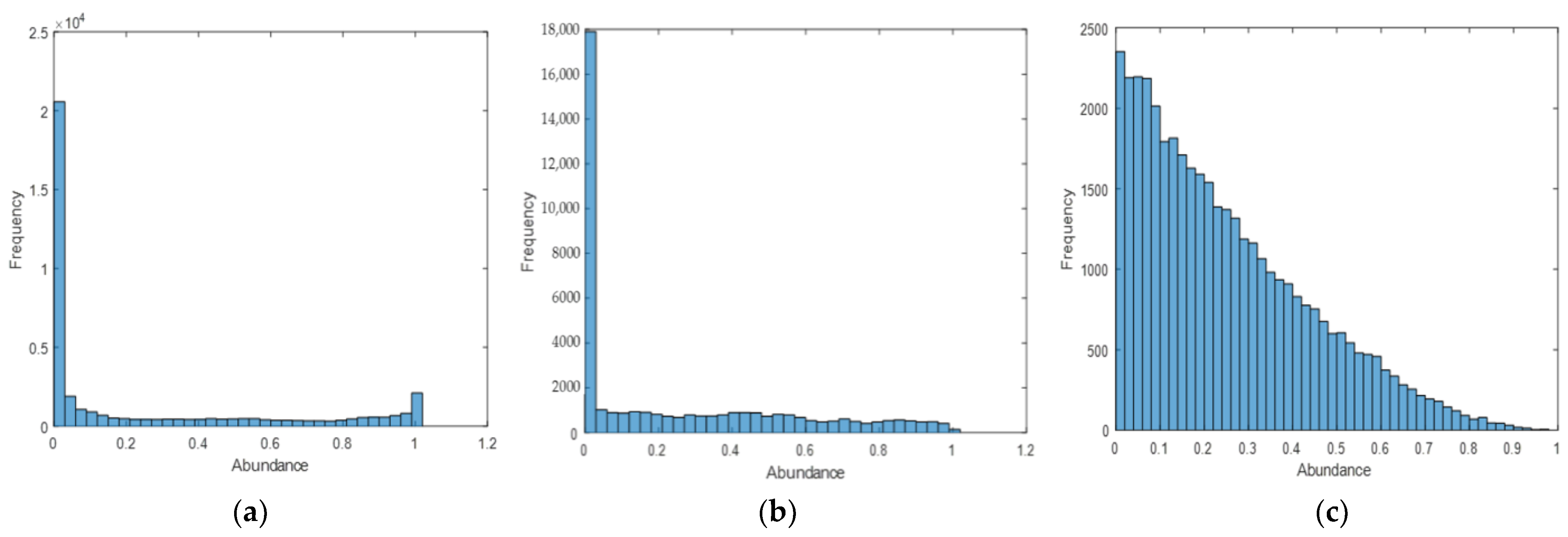
Firstly, a certain number of endmembers from the United States Geological Survey (USGS) digital spectrum library (Available here: http://speclab.cr.usgs.gov/spectral-lib.html (accessed on 1 February 2022)) are utilized to construct the endmember matrix E of the synthetic data. Each endmember contains 224 spectral bands, which are distributed between 0.38 and 2.5 μm. Since we already know the endmember matrix E , the bilinear endmember matrix F can be obtained easily. To generate the abundance matrix A , the method provided in the paper [50] is used, instead of using the Dirichlet distribution. From Figure 2, it can be found that the abundance produced by the method we use (Code is Available at: https://github.com/Growingg/Generate_data (accessed on 20 March 2022)) is sparser, and more similar to the abundance distribution of real HSI than that produced by the Dirichlet distribution. More specifically, we partition a known hyperspectral image into block regions, using super-pixel segmentation, and then randomly generate an abundance matrix that satisfies the ANC and ASC requirements for each block. The abundance matrix rank ranges from 1 to 4. Next, by setting the nonlinear coefficient γ between 0 and 1, the bilinear coefficient matrix B can be created. Finally, two kinds of noise are utilized to simulate the gaussian noise and impulse noise of real HSI:
  • Additive white Gaussian noise: Add Gaussian noise with a signal-to-noise ratio (SNR) of 30 dB for all bands;
  • Impulse noise: Add 20% Impulse noise to a 10% band, randomly selected.

4.1.1. Experiment on Synthetic Nonlinear Data and Linear Data

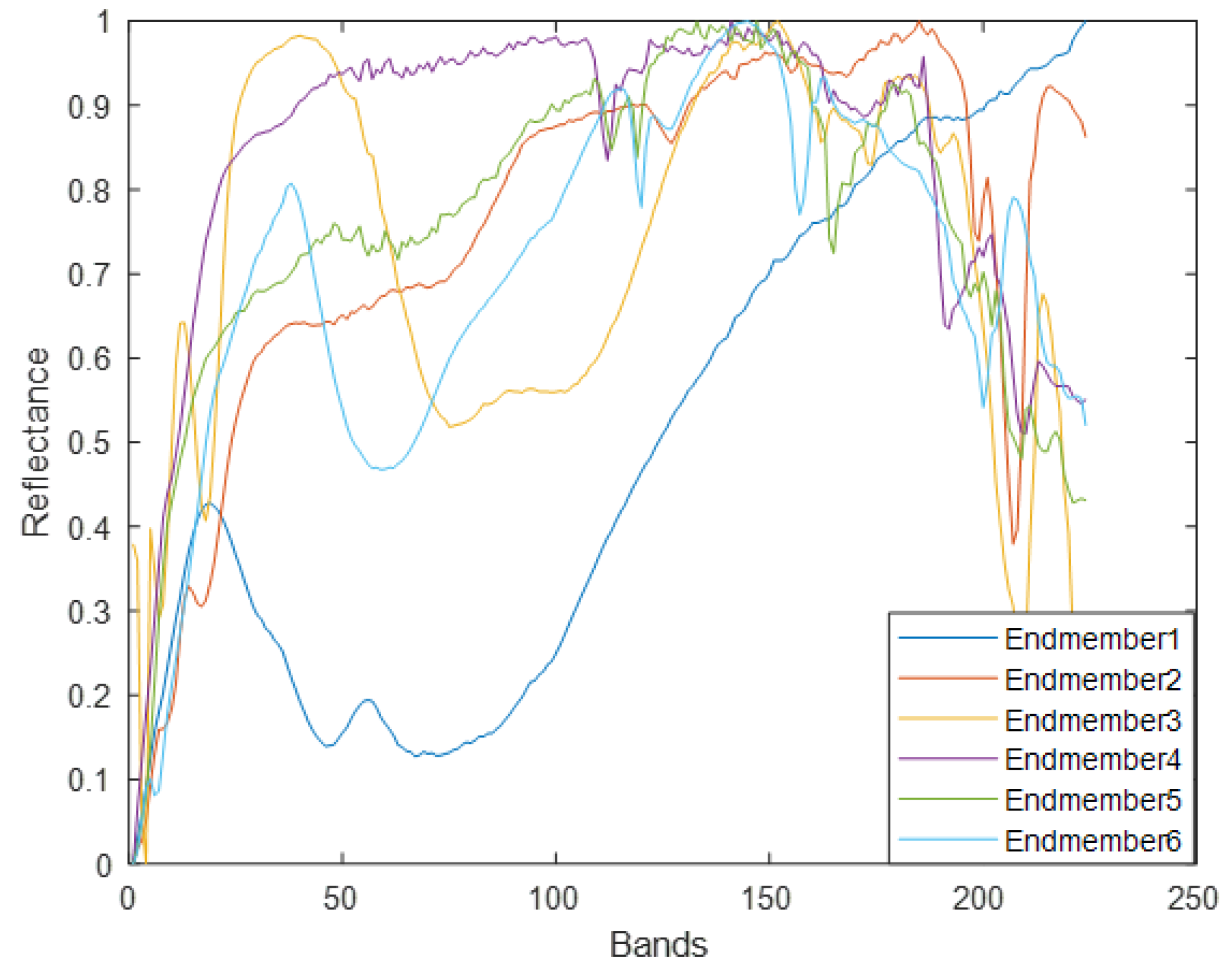
In this experiment, we synthesize both linear and nonlinear data with 6 endmembers using LMM and GBM under identical conditions. Figure 3 displays the six selected endmember spectral curves. For each synthetic image, a total of 10,000 pixels are generated. Both the rows and columns are 100. The parameters of the experiment are as follows: the input unit L is 224 and the encoder output unit M is 6. The learning rate is set to 10 4 and the batch size is 16.
Table 2 reports the performance of different methods on nonlinear mixed data. It can be seen that the nonlinear unmixing methods, i.e., MLM, FMAE, and GBM_AE, are superior to other linear unmixing methods. The proposed GBM_AE produces better results on all metrics than the other five approaches. Figure 4 shows the comparison of the six endmember spectra extracted by GBM_AE with the ground-truth endmembers spectra. The endmember spectra extracted by GMB_AE are very similar to the ground truth, indicating that GBM_AE performs well in endmember extraction. For the abundance estimation, our method obtains the lowest MSE and AAD. Figure 5 provides the visual comparison of the abundance maps obtained by all considered methods and ground-truth abundance maps. It can be noted that GBM_AE’s abundance maps are sparser than those obtained by other unmixing methods. In addition, the smallest RE demonstrates that GBM_AE can accurately reconstruct pixels in this nonlinear dataset.
The proposed GBM_AE also performs well on linear mixed data. From Table 3, we observe that, except for GBM_AE, the linear unmixing methods, i.e., MVCNMF, SUnSAL, and LinearAE, outperform other nonlinear unmixing methods. The proposed GBM_AE achieves the smallest MSE and SAD. In addition, the RE of GBM_AE is also relatively small, compared with other nonlinear methods. The nonlinear part of GBM_AE can be adjusted by the coefficient γ , and a small γ would be learned after training by linear data. This makes our method more flexible than other nonlinear unmixing methods and still achieves competitive performance on linear data. MVCNMF obtain the second smallest SAD, illustrating that the minimum volume constraint is beneficial for endmember extraction in the linear mixture scene.

4.1.2. Effect of the Endmember Number

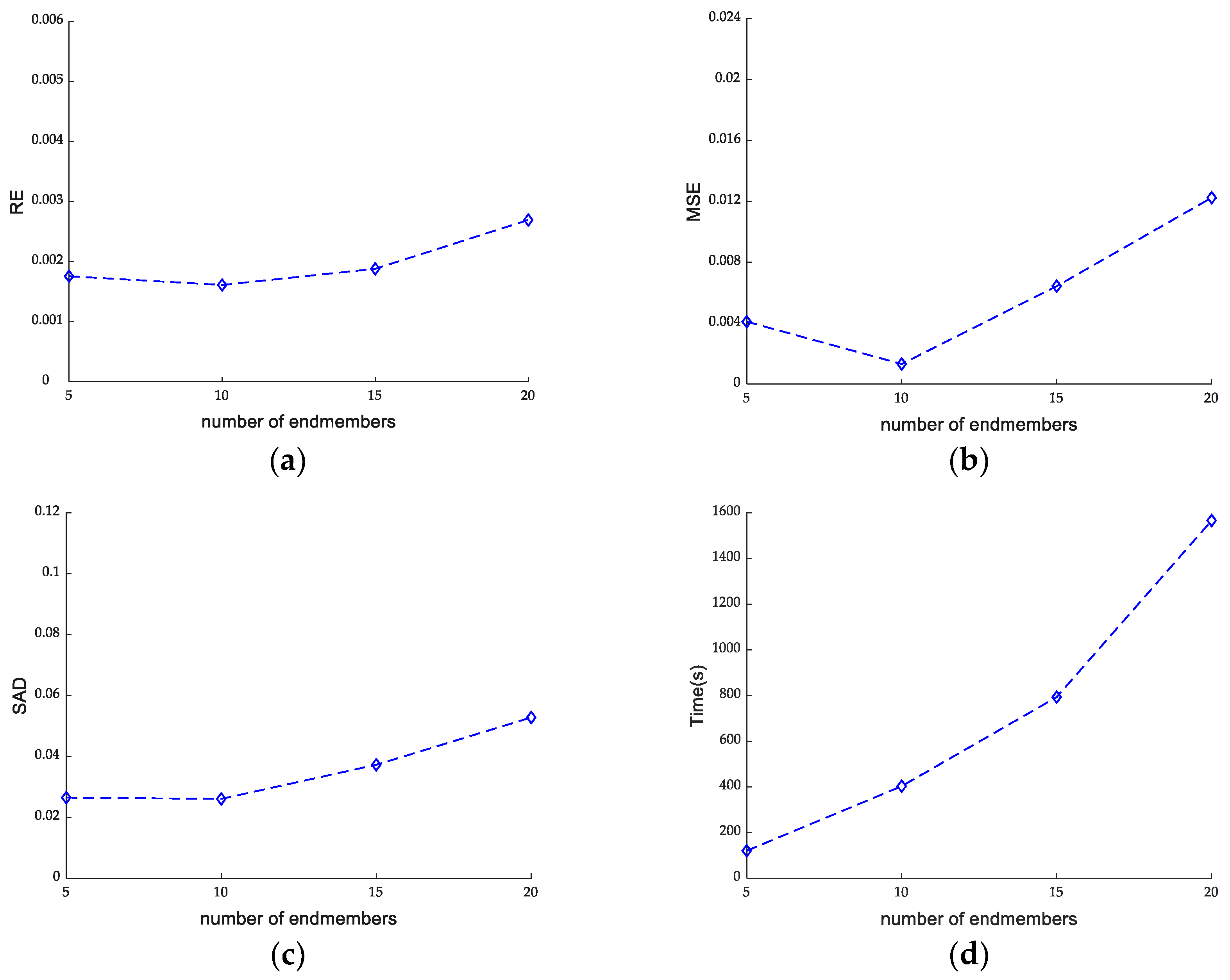
In this subsection, we conduct a study to assess the effect of the endmember number on the unmixing performance. In the experiment, the number of endmembers in nonlinear synthetic data varies from 5 to 20. Figure 6 shows the performance of GBM_AE as a function of the number of endmembers. In terms of RE, as the number of endmembers ( M ) increases, the reconstruction error does not change much. In terms of MSE and SAD, it can be observed that when the number of endmembers is relatively large, the value of MSE and SAD just decreases slightly. This means that the unmixing performance of the proposed GBM_AE is not fatally affected. Regarding running time, it exhibits an approximate quadratic relationship with M . To sum up, the number of endmembers alone has little effect on the performance of GBM_AE, but the computational cost of GBM_AE is greatly affected by the number of endmembers.

4.2. Experiments on Real Data

4.2.1. Jasper Ridge

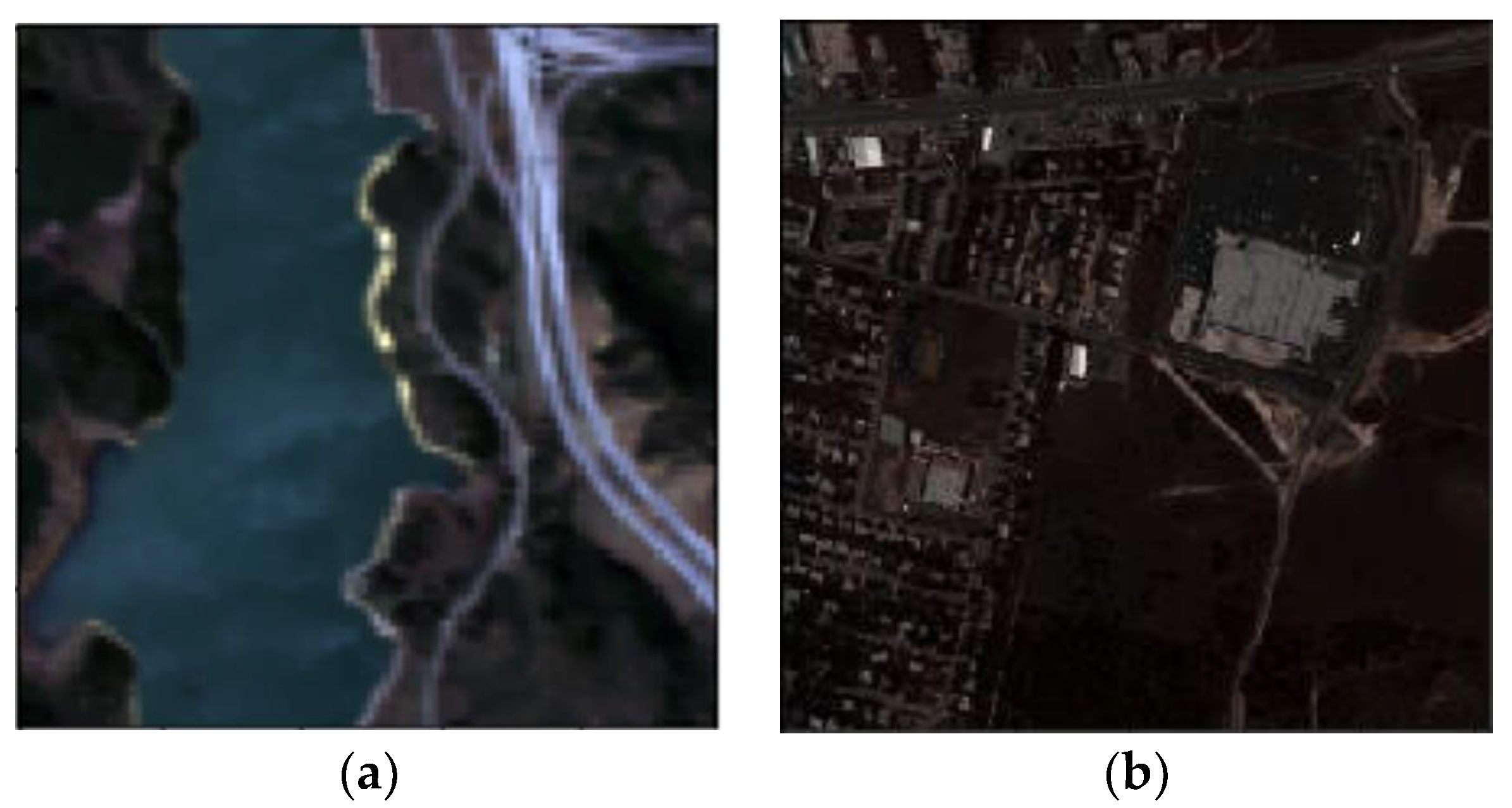
Jasper Ridge, a common hyperspectral data with 512 × 614 pixels, is widely used for hyperspectral processing. Each pixel is recorded at 224 channels with a spectral resolution of up to 10 nm, ranging from 400 nm to 2500 nm. In this experiment, a sub-image of 100 × 100 pixels with ground truth labeling is considered. The false color image of the chosen Jasper Ridge can be seen in Figure 7a. Removing the noisy bands that are contaminated with water vapor density and atmosphere, 198 channels are kept. There are four endmembers in this dataset: road, soil, water, and tree. The parameters of the experiment are as follows: the input unit L is 198 and the encoder output unit M is 4. The learning rate is set to 10 4 and the batch size is 20.
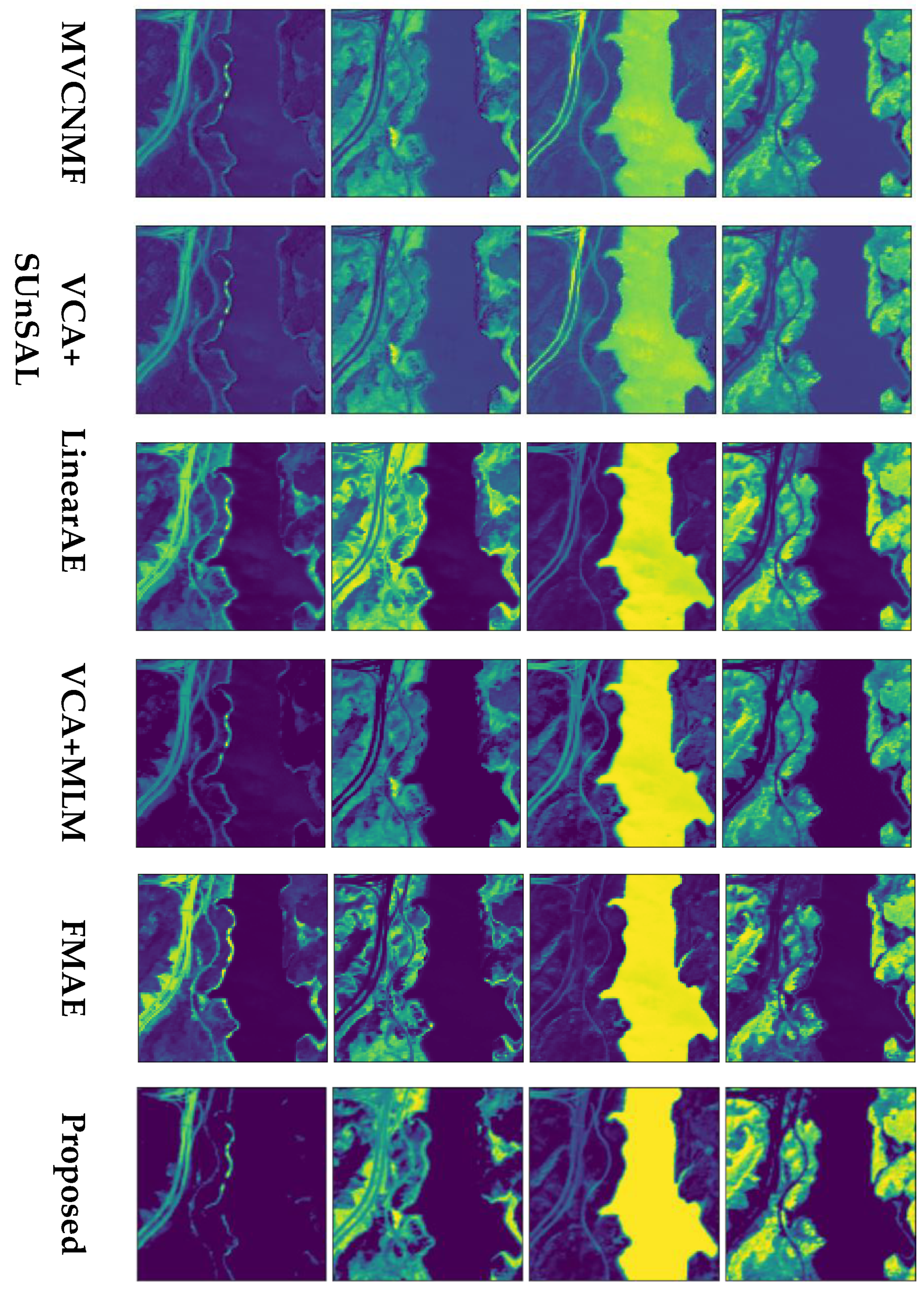
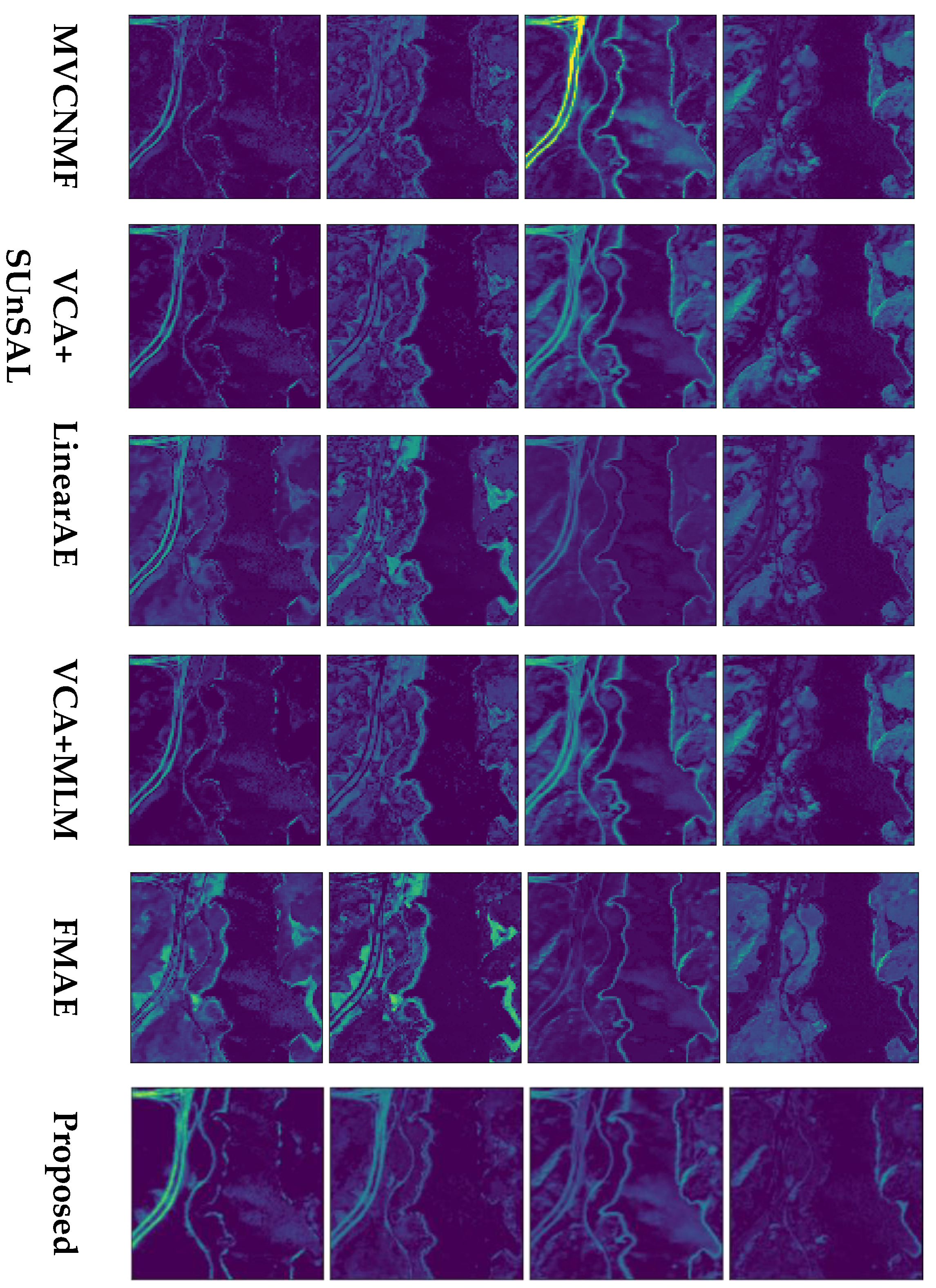
In the real HSIs, there is no doubt that the linear mixing and nonlinear mixing pixels exist at the same time. From Table 4, it can be observed that the performances of other linear or nonlinear methods are very similar, while the proposed GBM_AE shows obvious improvement. For SAD, GBM_AE is significantly better than other methods, indicating the superior performance of GBM_AE in endmember extraction. Figure 8 shows the comparison of endmember spectra extracted by GBM_AE with the reference one. As can be seen, the road has a somewhat worse spectral signature than the tree, water, and dirt. The reason may be that the road material is underrepresented in the Jasper Ridge dataset. For abundance estimation, GBM_AE achieves the lowest MSE and AAD, reflecting the fact that abundance maps estimated by GBM_AE are closest to the references. To make a visual assessment, Figure 9 depicts the abundance maps estimated by different methods and the reference abundance maps. We observe that the abundance maps estimated by MVCNMF and SUnSAL are not sparse enough. In addition, the soil and tree maps of GBM_AE contain more edge and detailed information, and are closer to the references than other compared methods. For further observation, we also show the difference maps between the abundance maps estimated by different methods and the reference abundance maps in Figure 10. It is evident that the difference is mainly concentrated at the boundary, and GBM_AE has a small value in difference maps of tree and soil. For the road map, it can be seen that our method has sharper lines and textures than other methods. Additionally, GBM_AE and other methods work equally on water, and the road may be misidentified as water. Figure 11 depicts the maps of the nonlinear factor γ ; the value of γ differs in different areas because it is obtained according to the forward propagation of the pixel itself. Nonlinear interactions are more likely to occur in the zone of contact between distinct components [33], and in maps of γ , i.e., a road-tree map, road-soil map and water-soil map, the value is relatively larger in the boundary areas between distinct materials. This shows that adaptive gamma values can be learned from GBM_AE. In summary, GBM_AE has significant potential for the unmixing of real HSI where both linear and nonlinear mixtures exist simultaneously.

4.2.2. Urban

The Urban dataset has been extensively studied in hyperspectral unmixing. The original dataset consists of 307 × 307 pixels, with each pixel corresponding to a 2 × 2 m2 ground area. There are 210 bands, ranging from 400 nm to 2500 nm, in each pixel. Because of the steam and air pollution, 162 bands are kept after removing the corrupted band. The false color image of Urban can be seen in Figure 7b. There are five materials in the observed scene: asphalt road, grass, tree, roof, and dirt. The experimental parameters are as follows: the input unit L is 162 and the encoder output unit M is 5. The learning rate is set to 10 4 and the batch size is 6.
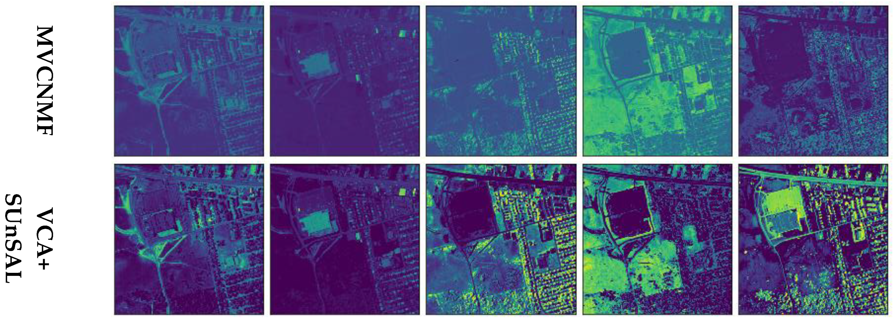
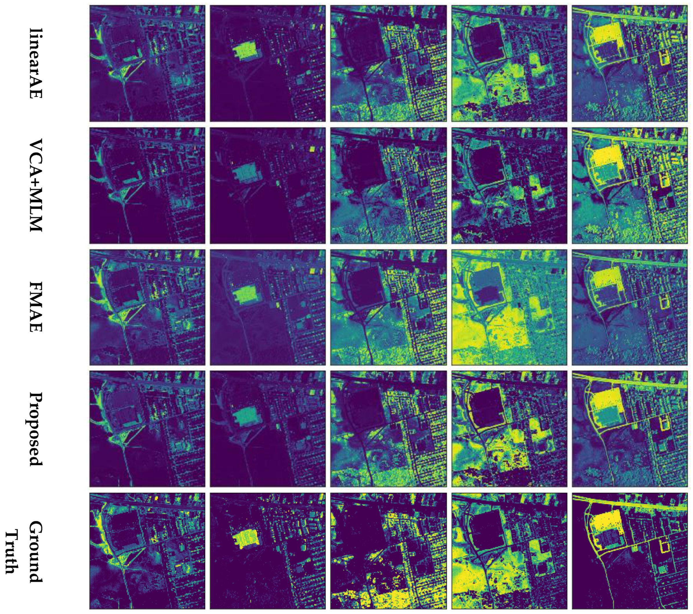
Table 5 shows the performance of all the considered methods on Urban. It can be seen that learning-based methods, i.e., LinearAE, FAE, and GBM_AE, are significantly better than traditional methods in general. For the quality of extracted endmember, GBM_AE has the lowest SAD, and Figure 12 shows that the endmember spectra extracted by GBM_AE are very similar to the references. In the terms of MSE and AAD, the proposed GBM_AE outperforms other compared approaches, which reflects the fact that GBM_AE has great advantages in estimating abundance. Figure 13 presents the abundance maps estimated by all methods. For reconstruction, both FMAE and GBM_AE have the smallest RE, and the MLM also obtain smaller RE than the other linear methods. These results indicate that it may be more competitive to consider nonlinear mixing effects on Urban dataset.

4.2.3. AVIRIS Cuprite

The hyperspectral image used in this subsection is the Cuprite dataset of Nevada, which is obtained by the well-known Airborne Visible Infrared Imaging Spectrometer (AVIRIS). Due to high similarity in materials spectra, Cuprite is the most widely used and challenging benchmark for HU research [51]. It has 400 × 350 pixels and 224 wavelength bands, ranging from 0.36 to 2.48 μm. Because of the effects of water absorption and low SNR, a total of 188 spectral bands are left after removing bands 1–2, 105–115, 150–170, and 223–224. In the experiment, a subset of 250 × 191 × 188 is considered, as shown in Figure 14. Regarding the endmembers in this subset, the researchers have their own thoughts, resulting in different versions of ground truths. Here, the version of 12 endmembers are chosen as the reference endmember, as in some previous studies [1,52]. The materials in cuprite include alunite, andradite, buddingtonite, dumortierite, kaolinite1, kaolinite2, muscovite, montmorillonite, nontronite, pyrope, sphene, and chalcedony. The experimental parameters are as follows: the input unit L is 188 and the encoder output unit M is 12. The learning rate is set to 10 4 and the batch size is 30.
Since the reference abundance of cuprite is unavailable, Table 6 only shows the obtained SAD and RE results from different methods. It can be seen that GBM_AE outperforms other methods on both SAD and RE. Figure 15 shows the 12 endmember spectral signatures extracted by GBM_AE compared with the references. In general, the endmember spectral signatures obtained by GBM_AE match well with the references. The number of abundance maps obtained by algorithms is 12, but some materials have very little distribution on the HSI, and the corresponding abundance map is difficult to observe with the naked eye. For observation and analysis, we show only the abundance maps of four materials with relatively clear images in Figure 16. The corresponding materials from left to right are sphere, dumortierite, buddingtonite, and nontronite. The proposed GBM_AE provides clearer maps of several specific emphasis positions. In summary, these results show the effectiveness of GBM_AE in complex scenarios.

4.3. Computational Complexity

In this subsection, we discuss the running time of all the considered methods. The experiments are performed on the same computer configuration having an eight-core CPU (Intel Core i5 8300H) and 16 GB of memory. Table 7 reports the average running time over 5 runs carried out on each dataset. It can be noted that deep-learning-based methods generally take more time than traditional methods. The FMAE has to consider the time of pretraining for the nonlinear part, so it takes the most time. The LinearAE and GBM_AE perform with the same epoch and batch sizes, and it can be found that the time cost of GBM_AE relative to LinearAE increases with the number of endmembers.

5. Discussion

It is generally known that the decoder of the autoencoder represents the spectral mixing process in HU tasks. Most of the autoencoder networks for blind unmixing are proposed for LMM without considering the nonlinearity of HSI, which will affect the unmixing accuracy in the real scene. In our work, we carefully designed a decoder based on the GBM, and promote the performance of unmixing.
Through experiments on synthetic nonlinear data, the proposed model outperforms comparison methods, which verifies the effectiveness of the proposed model. On synthetic linear data, even if not optimal on all metrics, the proposed method still shows competitive performance, because relatively small coefficient of the nonlinear part can be learned adaptively on linear mixing pixels to reduce the impact of nonlinear mixing part on spectral unmixing. This mean that it is an efficient extension of the linear model. In fact, not all materials have approximately linear reflective properties in real HSIs. Therefore, nonlinear and linear mixtures exist at the same time. In the experiments on real datasets, compared with traditional methods, GBM_AE borrows the powerful fitting ability and feature extraction ability of deep learning, and this helps to achieve a better performance. Compared with other nonlinear AEs, the proposed model considers only the second-order interaction, thus it is a relatively inexpensive nonlinear unmixing model. In addition, to avoid overfitting and obtaining the wrong estimated abundance and endmember, some regular constraint terms based on prior knowledge are constructed and added to the loss function of the network, e.g., SAD, and L 1 / 2 . In addition, the decoder of the proposed model is completely constructed according to the GBM, and the nonlinear factors γ of second-order interaction terms are obtained by forward propagation of pixels, which means that interpretable γ can be learned according to the feature of the input pixel after training, which greatly improves the adaptation of the proposed model.
Additionally, the method still has the following problems to be solved: (1) the unmixing accuracy and computational efficiency can still be further optimized and improved; (2) the interpretability of the network needs to be explored further; (3) it can be extended by introducing effective constraints such as noise reduction and spatial information.
All in all, we have effectively combined a traditional nonlinear mixing model GBM with deep learning techniques for nonlinear unmixing. This type of unmixing method may be a trend towards solving the mixed pixel issue in the future.

6. Conclusions

In this paper, an autoencoder network based on GBM is proposed for unmixing problems. This method is applied to a general mixing model composed of a linear mixed component and a nonlinear mixed component, and the endmembers and abundance are obtained simultaneously. We implement two custom layers to meet the requirements of abundance constraints and bilinear interactions, respectively. In order to improve the performance of unmixing, SAD and L 1 / 2 sparse regularization terms are introduced into the loss function. In particular, compared with other nonlinear approaches, the nonlinear mixing component in the proposed model can be adjusted by a set of learnable parameters, which enables the method to perform well on linear data, too. The comparative study on synthetic data and real hyperspectral images verifies the superiority of the proposed method.
This proposed method still has space for improvement. For instance, the autoencoder’s feature extraction only takes a single pixel into account, and ignores the spatial structure of the hyperspectral image. Spatial information may positively promote the learning of nonlinear parts. To further improve performance, we may combine spectral-spatial information with unmixing techniques in the future.

Author Contributions

Conceptualization, J.Z.; methodology, J.Z.; software, J.Z. and C.S.; validation, X.Z., H.M. and L.W.; formal analysis, J.Z. and L.W.; investigation, X.Z. and H.M.; resources, J.Z.; data curation, J.Z. and C.S.; writing—original draft preparation, J.Z.; writing—review and editing, X.Z. and H.M.; visualization, J.Z.; supervision, X.Z., H.M. and X.C.; project administration, J.Z. and X.Z.; funding acquisition, X.Z. and X.C. All authors have read and agreed to the published version of the manuscript.

Funding

This work was supported in part by the National Natural Science Foundation of China under Grant 61877066, Aero-Science Fund under Grant 20175181013 and Science and technology plan project of Xi’an under Grant 21RGZN0010.

Data Availability Statement

The data presented in this study are available in this article.

Conflicts of Interest

The authors declare no conflict of interest.

References

  1. Bioucas-Dias, J.M.; Plaza, A.; Camps-Valls, G.; Scheunders, P.; Nasrabadi, N.; Chanussot, J. Hyperspectral Remote Sensing Data Analysis and Future Challenges. IEEE Geosci. Remote Sens. Mag. 2013, 1, 6–36. [Google Scholar] [CrossRef] [Green Version]
  2. Bioucas-Dias, J.M.; Plaza, A. An overview on hyperspectral unmixing: Geometrical, statistical, and sparse regression based approaches. In Proceedings of the 2011 IEEE International Geoscience and Remote Sensing Symposium, Vancouver, BC, Canada, 24–29 July 2011; pp. 1135–1138. [Google Scholar]
  3. Keshava, N.; Mustard, J.F. Spectral unmixing. IEEE Signal Process. Mag. 2002, 19, 44–57. [Google Scholar] [CrossRef]
  4. Iordache, M.-D.; Bioucas-Dias, J.M.; Plaza, A. Sparse Unmixing of Hyperspectral Data. IEEE Trans. Geosci. Remote Sens. 2011, 49, 2014–2039. [Google Scholar] [CrossRef] [Green Version]
  5. Dópido, I.; Gamba, P.; Plaza, A. Spectral unmixing-based post-processing for hyperspectral image classification. In Proceedings of the 2013 5th Workshop on Hyperspectral Image and Signal Processing: Evolution in Remote Sensing (WHISPERS), Gainesville, FL, USA, 26–28 June 2013; pp. 1–4. [Google Scholar]
  6. Andrejchenko, V.; Heylen, R.; Scheunders, P.; Philips, W.; Liao, W. Classification of hyperspectral images with very small training size using sparse unmixing. In Proceedings of the 2016 IEEE International Geoscience and Remote Sensing Symposium (IGARSS), Beijing, China, 10–15 July 2016; pp. 5115–5117. [Google Scholar]
  7. Ibarrola-Ulzurrun, E.; Drumetz, L.; Chanussot, J.; Marcello, J.; Gonzalo-Martin, C. Classification Using Unmixing Models in Areas With Substantial Endmember Variability. In Proceedings of the 2018 9th Workshop on Hyperspectral Image and Signal Processing: Evolution in Remote Sensing (WHISPERS), Amsterdam, The Netherlands, 23–26 September 2018; pp. 1–4. [Google Scholar]
  8. Hou, S.; Shi, H.; Cao, X.; Zhang, X.; Jiao, L. Hyperspectral Imagery Classification Based on Contrastive Learning. IEEE Trans. Geosci. Remote Sens. 2022, 60, 1–13. [Google Scholar] [CrossRef]
  9. Yokoya, N.; Iwasaki, A. Effect of unmixing-based hyperspectral super-resolution on target detection. In Proceedings of the 2014 6th Workshop on Hyperspectral Image and Signal Processing: Evolution in Remote Sensing (WHISPERS), Lausanne, Switzerland, 24–27 June 2014; pp. 1–4. [Google Scholar]
  10. Ziemann, A.K. Local spectral unmixing for target detection. In Proceedings of the 2016 IEEE Southwest Symposium on Image Analysis and Interpretation (SSIAI), Santa Fe, NM, USA, 6–8 March 2016; pp. 77–80. [Google Scholar]
  11. Glenn, T.; Dranishnikov, D.; Gader, P.; Zare, A. Subpixel target detection in hyperspectral imagery using piece-wise convex spatial-spectral unmixing, possibilistic and fuzzy clustering, and co-registered LiDAR. In Proceedings of the 2013 IEEE International Geoscience and Remote Sensing Symposium-IGARSS, Melbourne, Australia, 21–26 July 2013; pp. 1063–1066. [Google Scholar]
  12. Ma, J.; Zhou, H.; Zhao, J.; Gao, Y.; Jiang, J.; Tian, J. Robust Feature Matching for Remote Sensing Image Registration via Locally Linear Transforming. IEEE Trans. Geosci. Remote Sens. 2015, 53, 6469–6481. [Google Scholar] [CrossRef]
  13. Cui, S.; Zhong, Y.; Ma, A.; Zhang, L. A novel robust feature descriptor for multi-source remote sensing image registration. In Proceedings of the IGARSS 2019—2019 IEEE International Geoscience and Remote Sensing Symposium, Yokohama, Japan, 28 July–2 August 2019; pp. 919–922. [Google Scholar]
  14. Guo, Q.; He, M.; Li, A. High-Resolution Remote-Sensing Image Registration Based on Angle Matching of Edge Point Features. IEEE J. Sel. Top. Appl. Earth Obs. Remote Sens. 2018, 11, 2881–2895. [Google Scholar] [CrossRef]
  15. Bioucas-Dias, J.M.; Plaza, A.; Dobigeon, N.; Parente, M.; Du, Q.; Gader, P.; Chanussot, J. Hyperspectral Unmixing Overview: Geometrical, Statistical, and Sparse Regression-Based Approaches. IEEE J. Sel. Top. Appl. Earth Obs. Remote Sens. 2012, 5, 354–379. [Google Scholar] [CrossRef] [Green Version]
  16. Veganzones, M.A.; Drumetz, L.; Tochon, G.; Dalla Mura, M.; Plaza, A.; Bioucas-Dias, J.; Chanussot, J. A new extended linear mixing model to address spectral variability. In Proceedings of the 2014 6th Workshop on Hyperspectral Image and Signal Processing: Evolution in Remote Sensing (WHISPERS), Lausanne, Switzerland, 24–27 June 2014; pp. 1–4. [Google Scholar]
  17. Drumetz, L.; Veganzones, M.A.; Henrot, S.; Phlypo, R.; Chanussot, J.; Jutten, C. Blind Hyperspectral Unmixing Using an Extended Linear Mixing Model to Address Spectral Variability. IEEE Trans. Image Process. 2016, 25, 3890–3905. [Google Scholar] [CrossRef] [PubMed] [Green Version]
  18. Xu, M.; Zhang, L.; Du, B.; Zhang, L. The linear mixed model constrained particle swarm optimization for hyperspectral endmember extraction from highly mixed data. In Proceedings of the 2016 8th Workshop on Hyperspectral Image and Signal Processing: Evolution in Remote Sensing (WHISPERS), Los Angeles, CA, USA, 21–24 August 2016; pp. 1–4. [Google Scholar]
  19. Miao, L.; Qi, H. Endmember Extraction From Highly Mixed Data Using Minimum Volume Constrained Nonnegative Matrix Factorization. IEEE Trans. Geosci. Remote Sens. 2007, 45, 765–777. [Google Scholar] [CrossRef]
  20. Nascimento, J.M.P.; Dias, J.M.B. Vertex component analysis: A fast algorithm to unmix hyperspectral data. IEEE Trans. Geosci. Remote Sens. 2005, 43, 898–910. [Google Scholar] [CrossRef]
  21. Afonso, M.V.; Bioucas-Dias, J.M.; Figueiredo, M.A. An augmented Lagrangian approach to the constrained optimization formulation of imaging inverse problems. IEEE Trans. Image Process. 2011, 20, 681–695. [Google Scholar] [CrossRef] [PubMed] [Green Version]
  22. Bioucas-Dias, J.M.; Figueiredo, M.A. Alternating direction algorithms for constrained sparse regression: Application to hyperspectral unmixing. In Proceedings of the 2010 2nd Workshop on Hyperspectral Image and Signal Processing: Evolution in Remote Sensing, Reykjavik, Iceland, 14–16 June 2010; pp. 1–4. [Google Scholar]
  23. Heinz, D.C.; Chein, I.C. Fully constrained least squares linear spectral mixture analysis method for material quantification in hyperspectral imagery. IEEE Trans. Geosci. Remote Sens. 2001, 39, 529–545. [Google Scholar] [CrossRef] [Green Version]
  24. Izquierdo-Verdiguier, E.; Gomez-Chova, L.; Bruzzone, L.; Camps-Valls, G. Semisupervised Kernel Feature Extraction for Remote Sensing Image Analysis. IEEE Trans. Geosci. Remote Sens. 2014, 52, 5567–5578. [Google Scholar] [CrossRef]
  25. Mateo-García, G.; Laparra, V.; Gómez-Chova, L. Optimizing Kernel Ridge Regression for Remote Sensing Problems. In Proceedings of the IGARSS 2018—2018 IEEE International Geoscience and Remote Sensing Symposium, Valencia, Spain, 22–27 July 2018; pp. 4007–4010. [Google Scholar]
  26. Hapke, B. Bidirectional reflectance spectroscopy: 1. Theory. J. Geophys. Res. Solid Earth 1981, 86, 3039–3054. [Google Scholar] [CrossRef] [Green Version]
  27. Hapke, B.; Wells, E. Bidirectional reflectance spectroscopy: 2. Experiments and observations. J. Geophys. Res. Solid Earth 1981, 86, 3055–3060. [Google Scholar] [CrossRef]
  28. Chen, W.; Cao, C.; Zhang, H.; Jia, H.; Ji, W.; Xu, M.; Gao, M.; Ni, X.; Zhao, J.; Zheng, S. Estimation of shrub canopy cover based on a geometric-optical model using HJ-1 data. In Proceedings of the 2011 IEEE International Geoscience and Remote Sensing Symposium, Vancouver, BC, Canada, 24–29 July 2011; pp. 1922–1925. [Google Scholar]
  29. Altmann, Y.; Dobigeon, N.; Tourneret, J.-Y. Bilinear models for nonlinear unmixing of hyperspectral images. In Proceedings of the 2011 3rd Workshop on Hyperspectral Image and Signal Processing: Evolution in Remote Sensing (WHISPERS), Lisbon, Portugal, 6–9 June 2011; pp. 1–4. [Google Scholar]
  30. Nascimento, J.M.; Bioucas-Dias, J.M. Nonlinear mixture model for hyperspectral unmixing. In Proceedings of the Image and Signal Processing for Remote Sensing XV, Berlin, Germany, 31 August–3 September 2009; pp. 157–164. [Google Scholar]
  31. Fan, W.; Hu, B.; Miller, J.; Li, M. Comparative study between a new nonlinear model and common linear model for analysing laboratory simulated-forest hyperspectral data. Int. J. Remote Sens. 2009, 30, 2951–2962. [Google Scholar] [CrossRef]
  32. Halimi, A.; Altmann, Y.; Dobigeon, N.; Tourneret, J.-Y. Nonlinear Unmixing of Hyperspectral Images Using a Generalized Bilinear Model. IEEE Trans. Geosci. Remote Sens. 2011, 49, 4153–4162. [Google Scholar] [CrossRef] [Green Version]
  33. Halimi, A.; Altmann, Y.; Dobigeon, N.; Tourneret, J.-Y. Unmixing hyperspectral images using the generalized bilinear model. In Proceedings of the 2011 IEEE International Geoscience and Remote Sensing Symposium, Vancouver, BC, Canada, 24–29 July 2011; pp. 1886–1889. [Google Scholar]
  34. Yokoya, N.; Chanussot, J.; Iwasaki, A. Nonlinear Unmixing of Hyperspectral Data Using Semi-Nonnegative Matrix Factorization. IEEE Trans. Geosci. Remote Sens. 2014, 52, 1430–1437. [Google Scholar] [CrossRef] [Green Version]
  35. Plaza, J.; Plaza, A.J.; Martinez, P.; Perez, R.M. Nonlinear mixture models for analyzing laboratory simulated-forest hyperspectral data. In Proceedings of the Image and Signal Processing for Remote Sensing IX, Barcelona, Spain, 9–12 September 2003; pp. 480–487. [Google Scholar]
  36. Licciardi, G.A.; Del Frate, F. Pixel Unmixing in Hyperspectral Data by Means of Neural Networks. IEEE Trans. Geosci. Remote Sens. 2011, 49, 4163–4172. [Google Scholar] [CrossRef]
  37. Zhang, X.; Sun, Y.; Zhang, J.; Wu, P.; Jiao, L. Hyperspectral Unmixing via Deep Convolutional Neural Networks. IEEE Geosci. Remote Sens. Lett. 2018, 15, 1755–1759. [Google Scholar] [CrossRef]
  38. Su, Y.; Li, J.; Plaza, A.; Marinoni, A.; Gamba, P.; Chakravortty, S. DAEN: Deep Autoencoder Networks for Hyperspectral Unmixing. IEEE Trans. Geosci. Remote Sens. 2019, 57, 4309–4321. [Google Scholar] [CrossRef]
  39. Palsson, B.; Ulfarsson, M.O.; Sveinsson, J.R. Convolutional autoencoder for spatial-spectral hyperspectral unmixing. In Proceedings of the IGARSS 2019—2019 IEEE International Geoscience and Remote Sensing Symposium, Yokohama, Japan, 28 July–2 August 2019; pp. 357–360. [Google Scholar]
  40. Min, A.; Guo, Z.; Li, H.; Peng, J. JMnet: Joint Metric Neural Network for Hyperspectral Unmixing. IEEE Trans. Geosci. Remote Sens. 2022, 60, 5505412. [Google Scholar] [CrossRef]
  41. Wang, M.; Zhao, M.; Chen, J.; Rahardja, S. Nonlinear Unmixing of Hyperspectral Data via Deep Autoencoder Networks. IEEE Geosci. Remote Sens. Lett. 2019, 16, 1467–1471. [Google Scholar] [CrossRef]
  42. Su, Y.; Xu, X.; Li, J.; Qi, H.; Gamba, P.; Plaza, A. Deep Autoencoders With Multitask Learning for Bilinear Hyperspectral Unmixing. IEEE Trans. Geosci. Remote Sens. 2021, 59, 8615–8629. [Google Scholar] [CrossRef]
  43. Li, H.; Borsoi, R.A.; Imbiriba, T.; Closas, P.; Bermudez, J.C.M.; Erdogmus, D. Model-Based Deep Autoencoder Networks for Nonlinear Hyperspectral Unmixing. IEEE Geosci. Remote Sens. Lett. 2022, 19, 5506105. [Google Scholar] [CrossRef]
  44. Dobigeon, N.; Tourneret, J.-Y.; Richard, C.; Bermudez, J.C.M.; McLaughlin, S.; Hero, A.O. Nonlinear Unmixing of Hyperspectral Images: Models and Algorithms. IEEE Signal Process. Mag. 2014, 31, 82–94. [Google Scholar] [CrossRef] [Green Version]
  45. Ioffe, S.; Szegedy, C. Batch Normalization: Accelerating Deep Network Training by Reducing Internal Covariate Shift. In Proceedings of the 32nd International Conference on Machine Learning, Lille, France, 6–11 July 2015; pp. 448–456. [Google Scholar]
  46. Keskar, N.S.; Mudigere, D.; Nocedal, J.; Smelyanskiy, M.; Tang, P.T.P. On large-batch training for deep learning: Generalization gap and sharp minima. arXiv 2016, arXiv:1609.04836. [Google Scholar]
  47. Masters, D.; Luschi, C. Revisiting small batch training for deep neural networks. arXiv 2018, arXiv:1804.07612. [Google Scholar]
  48. Palsson, B.; Sigurdsson, J.; Sveinsson, J.R.; Ulfarsson, M.O. Hyperspectral Unmixing Using a Neural Network Autoencoder. IEEE Access 2018, 6, 25646–25656. [Google Scholar] [CrossRef]
  49. Wei, Q.; Chen, M.; Tourneret, J.-Y.; Godsill, S. Unsupervised Nonlinear Spectral Unmixing Based on a Multilinear Mixing Model. IEEE Trans. Geosci. Remote Sens. 2017, 55, 4534–4544. [Google Scholar] [CrossRef] [Green Version]
  50. Mei, X.; Ma, Y.; Li, C.; Fan, F.; Huang, J.; Ma, J. Robust GBM hyperspectral image unmixing with superpixel segmentation based low rank and sparse representation. Neurocomputing 2018, 275, 2783–2797. [Google Scholar] [CrossRef]
  51. Zhu, F. Hyperspectral unmixing: Ground truth labeling, datasets, benchmark performances and survey. arXiv 2017, arXiv:1708.05125. [Google Scholar]
  52. Wang, X.; Zhong, Y.; Zhang, L.; Xu, Y. Blind Hyperspectral Unmixing Considering the Adjacency Effect. IEEE Trans. Geosci. Remote Sens. 2019, 57, 6633–6649. [Google Scholar] [CrossRef]
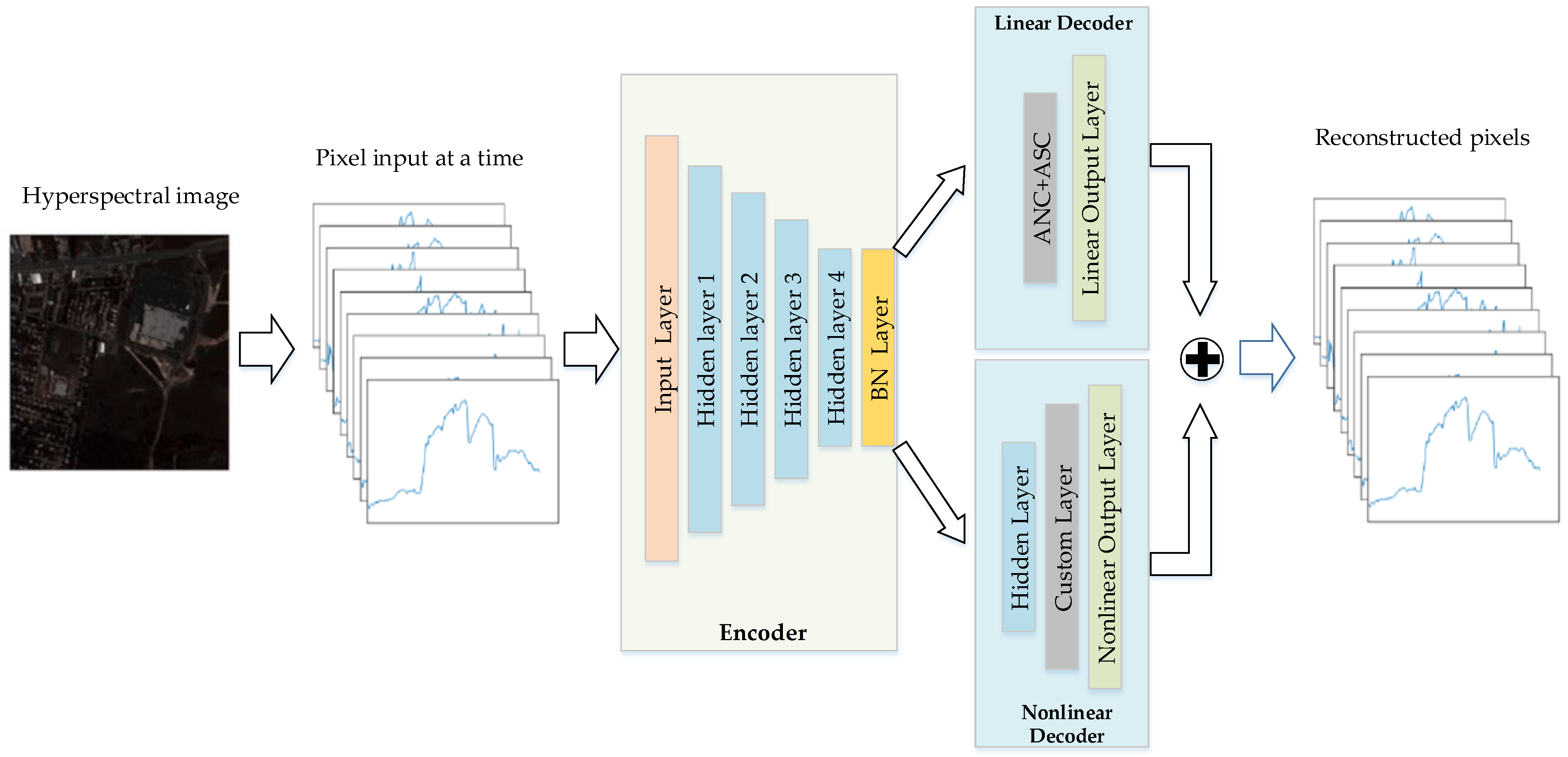
Figure 1. Structure of the Proposed Autoencoder Network based on GBM.
Remotesensing 14 05167 g001
Figure 2. Histogram distribution of abundance of (a) Jasper Ridge; (b) data generated by the method we use; (c) data generated by Dirichlet distribution.
Remotesensing 14 05167 g002
Figure 3. Six selected endmember spectral signatures in USGS.
Remotesensing 14 05167 g003
Figure 4. Comparison of the reference endmember (red line) with the endmember extracted by GBM_AE (blue line) on Nonlinear Mixed Data.
Remotesensing 14 05167 g004
Figure 5. Estimated abundance maps for Nonlinear Mixed Image. From left to right for different endmembers. From top to bottom for different methods.
Remotesensing 14 05167 g005
Figure 6. Performance of GBM_AE model as a function of the number of endmembers. (a) RE; (b) MSE for abundance; (c) SAD for endmember; (d) running time.
Remotesensing 14 05167 g006
Figure 7. False-color image of (a) Jasper Ridge, (b) Urban.
Remotesensing 14 05167 g007
Figure 8. Comparison of the reference endmember (red line) with the endmember extracted by GBM_AE (blue line) on Jasper Ridge. From left to right for different endmembers: tree, water, soil and road.
Remotesensing 14 05167 g008
Figure 9. Estimated abundance maps for Jasper Ridge. From left to right for different endmembers: road, soil, water and tree. From top to bottom for different methods.
Remotesensing 14 05167 g009aRemotesensing 14 05167 g009b
Figure 10. Abundance difference maps for Jasper Ridge. From left to right for different endmembers: road, soil, water and tree. From top to bottom for different methods.
Remotesensing 14 05167 g010
Figure 11. The maps of the gamma γ inferenced by GBM_AE on Jasper Ridge. From left to right for different second-order interaction terms: road-water, road-tree, road-soil, water-tree, water-soil and tree-soil.
Remotesensing 14 05167 g011
Figure 12. Comparison of the reference endmember (red line) with the endmember extracted by GBM_AE (blue line) on Urban. From left to right for different endmembers: asphalt, grass, tree, roof, and dirt.
Remotesensing 14 05167 g012
Figure 13. Estimated abundance maps for Urban. From left to right for different endmembers: dirt, roof, tree, grass and asphalt road. From top to bottom for different methods.
Remotesensing 14 05167 g013aRemotesensing 14 05167 g013b
Figure 14. False-color image of cuprite.
Remotesensing 14 05167 g014
Figure 15. Comparison of the reference endmember (red line) with the endmember extracted by GBM_AE (blue line) on cuprite. From left to right on the first row: alunite, andradite, buddingtonite, dumortierite, kaolinite1, kaolinite2; from left to right on the second row: muscovite, montmorillonite, nontronite, pyrope, sphene, and chalcedony.
Remotesensing 14 05167 g015
Figure 16. Estimated abundance maps for cuprite. The corresponding materials from left to right are: sphere, dumortierite, buddingtonite and nontronite. From top to bottom for different methods.
Remotesensing 14 05167 g016
Table 1. Structure of the Proposed Autoencoder Network for GBM.
LayersActivationUnitsBias
EncoderInput layer-LNo
Hidden layer 1Leaky ReLU9∗MNo
Hidden layer 2Leaky ReLU6∗MNo
Hidden layer 3Leaky ReLU3∗MNo
Hidden layer 4Leaky ReLUMNo
Batch Normalization-M-
DecoderLinear partANC + ASC-M-
Linear output layer-LNo
Nonlinear partHidden layer Ø M(M − 1)/2No
Custom layer-M(M − 1)/2No
Nonlinear output layer-LNo
Table 2. Comparison of different methods on Nonlinear Mixed Data. Best results are reported in bold.
MVCNMFVCA + SUnSALLinearAEVCA + MLMFMAEProposed
MSE0.01150.01470.01420.01100.01110.0030
AAD0.27640.29590.35110.26760.32110.1486
SAD0.07210.08010.07310.06720.09180.0377
RE0.00420.00310.00410.00680.00230.0019
Table 3. Comparison of different methods on Linear Mixed Data. Best results are reported in bold.
MVCNMFVCA + SUnSALLinearAEVCA + MLMFMAEProposed
MSE0.01120.01110.01070.01580.01200.0092
AAD0.27360.27310.29560.30350.31370.2921
SAD0.05870.08010.06430.08170.09110.0322
RE0.00030.00120.00540.00350.00590.0018
Table 4. Comparison of different methods on Jasper Ridge. Best results are reported in bold.
MVCNMFVCA + SUnSALLinearAEVCA + MLMFMAEProposed
MSE0.02640.02410.02160.02340.02600.0185
AAD0.46170.43000.42740.32460.43630.2134
SAD0.17730.17260.31610.24130.12750.0869
RE0.00290.00280.00300.00280.00220.0005
Table 5. Comparison of different methods on Urban. Best results are reported in bold.
MVCNMFVCA + SUnSALLinearAEVCA + MLMFMAEProposed
MSE0.07390.05730.04520.08640.05110.0336
AAD0.84520.67020.61040.75250.57510.4951
SAD0.30320.36410.20310.26670.19580.1908
RE0.00610.00580.00500.00470.00150.0015
Table 6. Comparison of different methods on cuprite. Best results are reported in bold.
MVCNMFVCA + SUnSALLinearAEVCA + MLMFMAEProposed
SAD0.11720.12120.13930.10520.10380.0937
RE3.41 ×   10 3 4.01 ×   10 3 1.54 ×   10 3 1.07 ×   10 3 7.56 ×   10 4 3.05 ×   10 4
Table 7. The average running time in second (s) for all methods on each dataset.
Syn
Linear
Syn
Nonlinear
Jasper RidgeUrban Cuprite
MVCNMF103439631559
VCA + SUnSAL11615
LinearAE686623028181
VCA + MLM128984873754
FMAE2032111175176774
GBM_AE14215455850689
Publisher’s Note: MDPI stays neutral with regard to jurisdictional claims in published maps and institutional affiliations.