Abstract
Accurate and error-free digital elevation model (DEM) data are a basic guarantee for the safe flight of unmanned aerial vehicles (UAVs) during surveys in the wild, especially in moun-tainous areas with large topographic undulations. Existing free and open-source DEM data gen-erally cover large areas, with relatively high spatial resolutions (~90, 30, and even 12.5 m), but they do not have the advantage of timeliness and cannot accurately reflect current and up-to-date topographical information in the survey area. UAV pre-scanning missions can provide highly accurate and recent terrain data as a reference for UAV route planning and ensure security for subsequent aerial survey missions; however, they are time consuming. In addition, being limited to the electric charge of the UAV, pre-scanning increases the human, financial, and time consumption of field missions, and it is not applicable for field aerial survey missions in reality, unless otherwise specified, especially in harsh environments. In this paper, we used interferometric synthetic aper-ture radar (InSAR) technology to process Sentinel-1a data to obtain the DEMs of the survey area, which were used for route planning, and other free and open-source DEMs were also used for flightline plans. The digital surface models (DSMs) were obtained from the structure of the UAV pre-scan mission images, applying structure for motion (SfM) technology as the elevation reference. Comparing the errors between the InSAR-derived DEMs and the four open-source DEMs based on the reference DSM to analyze the practicability of flight route planning, the results showed that among the four DEMs, the SRTM DEM with a spatial resolution of 30 m performed best, which was considered as the first reference for UAV route plans when the survey area in complex mountainous regions is covered with a poor or inoperative network. The InSAR-derived DEMs from the Sentinel-1 images have great potential value for UAV flight planning, with a large perpendicular baseline and short temporal baseline. This work quantitatively analyzed the errors among the different DEMs and provided a discussion regarding UAV flightline plans based on external DEMs. This can not only effectively reduce the manpower, materials, and time consumption of field operations, improving the efficiency of UAV survey tasks, but it also broadens the use of InSAR technology. Furthermore, with the launch of high-resolution SAR satellites, InSAR-derived DEMs with high spatial and temporal resolutions provide an optimistic and credible strategy for UAV route planning with small errors.
1. Introduction
As a new surveying and mapping technology, unmanned aerial vehicles (UAVs) loaded with a small camera have the advantages of being easy to carry and having high-resolution data acquisition (with spatial resolutions at the centimeter scale) [1,2,3]. Because of their unique “God perspective”, they capture scenes and characters that humans, owing to their ground-based line of sight, cannot, often resulting in exciting and shocking images and spectacles [4,5]. In addition, based upon the analysis of these images, they can dynamically look for ground surface features that were previously unknown or difficult to find. Due to the fact of these advantages and unique photographic visual properties, drones are widely used in the fields of ecological investigation and biomass estimation [6,7,8], basic surveying [9,10], agricultural subjects [11,12], scientific research and investigation [10,13], and rescue and emergency [14,15,16,17], and are increasingly more popular not only in scientific research but also in daily life (e.g., film and television shooting, and outdoor activities videoing).
In recent years, thanks to the steady development of UAV flight control technology and the continuous improvement of UAV battery capacity [6,18,19], an increasing number of industries have started to take advantage of UAVs as an alternative to traditional manual, high-risk operations, e.g., power line and steel tower inspections [20,21,22,23] and field surveys in harsh environments (e.g., complex mountainous terrains, polar environments, and very high- or extremely low-temperature surroundings) [24,25,26,27,28]. Powerful theoretical knowledge regarding the UAV and proficient operating skills are necessary for good UAV survey performance. Considering the complexity of unfamiliar environments and the natural features of mountains (e.g., meteorology, electromagnetic fields, light and reflection, topographic relief, distribution of ground structures, and environmental management) [29], pre-scanning flying work is needed. To obtain an accurate terrain dataset, which is then used as a reference for the subsequent aerial survey route planning for the drone to ensure operational safety, an advanced scanning flying mission is recommended, particularly in a high gradient topography region, Generally, UAV pre-scanning is based on free and open-source digital elevation model (DEM) data, which are usually packaged into the operation control system (OCS), similar to a “black box”, and we do not usually know what it contains. The data are auto-downloaded when the UAV operator is planning the flight routes if the OCS is online. If the survey areas are not covered (or poorly covered) by the internet communication, importing the external DEMs as a reference for UAV flightline planning is necessary and recommended. Hence, accurate and useful DEMs are fundamental in UAV route planning.
A digital elevation model (DEM) is the vertical distance between the ground surface and a reference datum, not including trees (i.e., forest canopy), buildings, etc., and it contains abundant information on landforms and terrain features [30], widely used for hydrology analysis and river extraction [31,32]. Another terrain representation referring to the uppermost surface of both topography and features is called a digital surface model (DSM), including buildings, tree canopy, and vegetation, which is usually what is seen on an aerial/satellite image or first-return pulse from a laser scanner [30]. With a high-altitude flight path and carrying a visible light lens, a UAV takes aerial photographs for surveying areas from the air to obtain coarse terrain data (DSM) and a ground features map (orthographic imagery). The main purpose of a pre-scanning task is to gain the exact DSM of the survey area, which is used in the following aerial survey mission to obtain higher-resolution UAV images. Therefore, DEM or DSM data are most critical for drone aerial surveys in complex mountainous surroundings.
Compared with existing open-source DEM datasets, the elevation information obtained by pre-scanning has great advantages in spatial resolution and timeliness [33,34]. In addition, a pre-scan is tantamount to familiarizing yourself with the new environment (since the flight altitude set during pre-scan is usually much higher than the difference in altitude between the takeoff point of the UAV and the highest point in the measured area, and there is little risk to the UAV hitting an obstacle during the flight). At the same time, the elevation data obtained are also an important basis for future flight path planning [29,35], especially in ground-level flight operations or areas without network coverage. However, an advance sweep usually requires a great deal of manpower, materials, and time and is not appropriate for field aerial surveys. How to obtain the latest and relatively accurate elevation data for current ground conditions is an urgent and fundamental problem [33,34,36].
InSAR has been developed for more than 40 years since its introduction [37], and it is one of the state-of-the-art technologies for elevation generation. With the successful launch of a growing number of SAR satellites, advances in computer hardware and software, and algorithms, InSAR has been successfully applied to monitor surface deformation caused by natural disasters, such as earthquakes, volcanic eruptions, glacier drift, and geological hazards, associated with human activities, e.g., landslides and ground subsidence [15,38,39,40,41,42,43,44,45]. In addition, InSAR technology can also be used for topographic mapping, and many researchers have conducted numerous studies on this topic with good results [34,36,37,46,47,48]. SAR imagery is highly capable of extracting surface topographic information due to its low impact on weather, the inclusion of phase information of features at the time of acquisition, and the short cycle of revisit period (e.g., 24 days for a single Sentinel-1 and 12 days for the double-constellation Sentinel-1a/b). The short revisit interval ensures that the surface deformation of the area covered by the two acquisitions closes to zero infinitely, thus ensuring that the phase difference is caused by the terrain itself, which is the base to DEM calculating. The opportunity to have up-to-date elevation data due to the continuous monitoring and activity of Sentinel-1.
Founded on the above description, a precise and recently created or produced terrain dataset is required for high-resolution images of the UAV survey. The DSM obtained from unmanned drone pre-scanning missions are usually good, but this task is time consuming and laborious, which are not appropriate for large survey areas, especially in harsh environments. To solve this issue, we analyzed the practicability of UAV route planning based on different DEMs. Concretely, recent elevation information, obtained from InSAR processing of Sentinel-1 data, has been used for UAV field surveys, which is intended as an alternative to pre-scanning. In this paper, terrain data of a complex mountain region were obtained from the Sentinel-1a InSAR processing and, at the same time, the DSM was also obtained from the UAV pre-scanning task. In addition, several open-source elevation products were collected. The DSM was regarded as the reference for the error analysis of the other elevation values, and the elevation data were used for the UAV route planning to select which one was best. We focused on validating the practicability of the UAV survey based on the elevation data obtained from the Sentinel-1 InSAR processing. This study not only expands the potential usage range of InSAR-derived elevation data obtained from Sentinel-1, but also has important implications for replacing pre-scanning efforts in complex mountain regions.
This paper is organized as follows: Section 2 provides an overview of the survey area: Zheduoshan Mountains, China. Section 3 introduces the data and methods used in this paper in detail. Section 4 presents the results including an analysis and visualization of the characteristics of the elevation errors and a feasibility analysis of the UAV route plans. In Section 5, we discuss the influencing factors of the InSAR-derived DEM processing and UAV flightline plans prior to presenting the concluding remarks in Section 6. In addition, to decrease misunderstandings regarding the elevation, in this paper, we addressed the elevation generated from UAV images only using the terminology “DSM”, and all other descriptions of elevation information were classified as “DEM”. Namely, we did not distinguish the connotations regarding DSM and DEM, and DSM was used just to indicate that it was produced from UAV images.
2. Overview of the Study Area
The survey area is located near the 318 National Highway by the Zheduoshan Mountains, Southwest China, with the geographical coordinates of 30°02′51.03″-30°06′32.74″N and 101°48′32.58″–101°52′36.84″E (Figure 1). Covering an area of 22.6 km2 and with a large rolling topography, one large WN–ES trending mountain range (Figure 1, the magenta rectangle) and two small WS–EN trending mountain ranges (Figure 1a, the magenta ellipse) are dominant. As a result of tectonic activity and Quaternary glacial drift, rocks have been subjected to severe weathering, and rockfalls and break stones are ubiquitous. In addition, the ground surface covers sparse vegetation [49], there are no trees, and existing transmission line towers are standing (Figure 1b and Figure 2c).
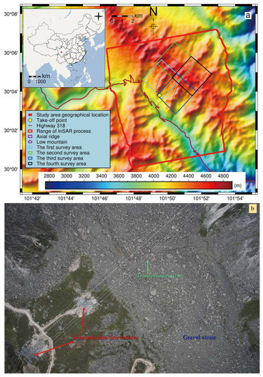
Figure 1.
A geographical overview of the study area: (a) the topography of the study area, based on the TerraSAR-X add-on for digital elevation measurement (TanDEM) and the study area within a larger map of China (Zheduoshan Mountain in Sichuan Province, China); and (b) a photo of the standing transmission line towers, mainly covered with gravel stone.
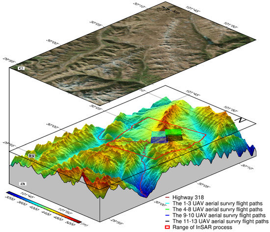
Figure 2.
Enlarged view of the study area: (a) a three-dimensional topographic view of the survey area based on the AOLS PALSAR DEM (12.5 m); (b) the InSAR processing area (polygon marked red) and the flight paths corresponding to the four subareas (the cyan, green, blue, and black lines represent block one, two, three, and four, respectively); and (c) the ground surface cover based on Google Map satellite images of the study area. All maps are at the 135/25 (azimuth/angle of pitch) view, differing in altitude.
The survey area is located in a subtropical monsoon climate region, with a rainy summer and snowy winter. The annual average temperature is approximately 9 °C, the extreme maximum temperature is 19.4 °C, and the extreme minimum temperature is −14.1 °C [50]. There are obvious seasonal repeated freezing and thawing phenomena at the ground surface due to the large thermal excursion between day and night, which happens in the winter period from November to March [51,52]. The frost action accelerates the natural weathering effect, which induces the bare rocky debris everywhere. The deformation velocity of this region is serious, ranging from −136.59 to 112. 86 mm per year [53].
In addition, due to the installation of transmission line towers, a large number of excavations have been conducted at the site (Figure 1b), which may aggravate the regional collapse of the mountain. The smoothness of the roads is a basic guarantee that ensures the stable operation of the circuit maintenance and other work at a later stage, and the large amounts of debris rolling down may induce an impact on the smoothness of the road, which needs more attention. Hence, it is necessary to conduct a large-scale aerial UAV survey in this region.
The pre-scanning aerial survey mission was carried out using an FeiMa Robotics D200 (sometimes called a D200s) multirotor UAV (https://www.feimarobotics.com/en/productDetailD200 (accessed on 28 August 2022)), equipped with a SONY ILCE-6000 camera and positioning with a single-base station and post-processed kinematic (PPK) mode technology. Figure 2 shows the UAV flight path of the area of interest including topography and land covering features. The flight routes were set at a fixed altitude of 510 m based on the ground sample distance (GSD) of 10 cm/pixel. The direction overlaps and side were 80% and 60%, respectively. Because of the large area of the aerial survey range, the UAV Butler flight management control system automatically divided the large survey area into four small blocks (Figure 1a, the four rectangular boxes colored cyan, green, blue, and black represent the black first, second, third, and fourth, respectively) with the corresponding four routes (Figure 2b, the color is the same as block boundary). Further, as the surface elevation of the survey area varied greatly (Figure 2a), the four tiles had different average elevation values, which induced the various absolute flight height of each block. Concretely, the absolute survey route heights of subregions 1st—4th were 4932, 5025, 4942, and 5057 m, respectively (Figure 2b). The sortie number per block varied from two to five, and a total of 13 flight sorties were conducted in the whole survey area (i.e., four blocks), capturing 1283 images (Table 1, Section 3). A high-precision DSM and orthographic map with a spatial resolution of 0.1 m can be obtained after the UAV image processing.

Table 1.
Detailed information on aerial photographs taken by drones in the survey area.
3. Data sources and Methodologies
3.1. Data Source
The UAV data collection dated from 25 to 26 August 2020 from the pre-scanning mission, with an equal flight height of 510 m; see Table 1 for details. This pre-scanning UAV aerial survey was carried out with a geographical positioning based on a single base station. The large survey area (22.6 km2) and the high-altitude flight paths of the pre-scanning efforts increased the consumption of time, which is not appropriate because of the intrinsic limited endurance of the UAV. It took two days to finish the pre-scanning mission, and a total of 13 aerial flights were conducted, obtaining 1283 images.
Sentinel-1a image data were downloaded from the European Space Agency (ESA, https://scihub.copernicus.eu/dhus/#/home (accessed on 1 July 2022)), and the corresponding precise orbit data were obtained from the Earth Data (https://s1qc.asf.alaska.edu (accessed on 1 July 2022)). Based on the acquisition date between the Sentinel-1a (no Sentinel-1b imagery was obtained) and UAV pre-scanning photographs and the location of the survey area, the optimal results of the two pairs of Sentinel-1a imageries (ascending and descending) were selected with the smaller temporal baseline (TB) and larger perpendicular baseline (PB) (Table 2). The PB was 84.54 and 31.87 m for the ascending and descending pair, respectively, and both TBs for them were the smallest interval at 12 days.
Table 2.
Information on the Sentinel-1a images.
The free and open-source DEM data used in this paper, including the ALOS PALSAR DEM, generated from the L-band SAR images (with a ground surface spatial resolution of 12.5 m, downloaded from: https://search.asf.alaska.edu (accessed on 1 July 2022)); SRTM 1-Arc DEM_V3 (Shuttle Radar Topography Mission, with a spatial resolution of 1Arc-Sec, approximately ~30 m, 3rd version, downloaded from: https://earthexplorer.usgs.gov (accessed on 1 July 2022)); ASTER GDEM_V003 (the ASTER Global Digital Elevation Model, with a spatial resolution of 1 arc second, approximate ~30 m, version 3, downloaded from: https://search.earthdata.nasa.gov (accessed on 1 July 2022)); and TanDEM (TanDEM-X-Digital Elevation Model, with the global earth’s landmasses from pole to pole, which had a reduced pixel spacing of 3 arcseconds, approximately 90 m at the equator, downloaded from: https://download.geoservice.dlr.de/TDM90 (accessed on 1 July 2022)), were collected. Above all, DEMs are usually generated from aerial surveys and satellite images with InSAR [54] and stereo pair measurement, but they are not representative of the most recent topography, because the land morphology is constantly changing due to the natural and human activities.
3.2. Methodologies
Data processing mainly includes three parts: the production of DEM products applying InSAR technology; the production of high-precision products (i.e., orthophoto and DSM) based on the UAV pre-scanning photographs; and the results of the analysis based on the elevation errors and flight heights. These three parts are detailed in Figure 3.
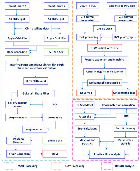
Figure 3.
Method flow chart including InSAR processing, UAV image processing, and subsequent data analysis. The tripartite auxiliary data as input are shown in green, and the resulting products are marked with red rectangular boxes. TOPS, terrain observation with progressive scan; SRTM 1 Sec, Shuttle Radar Topography Mission 1-arc Second V3.0 DEM; ROI, region of interest; DEM, digital elevation model; UAV, unmanned aerial vehicle; RTK, real-time kinematic; POS, position and orientation system; PPK, post-processed kinematic; GPS, global positioning system; EXIF, exchangeable image file format; DSM, digital surface model.
3.2.1. Sentinel-1 InSAR Processing for DEM Generation
Based on the phase recorded of the ground surface from SAR satellite images, the DEM can be obtained from InSAR technology [34,46,55]. InSAR processing with Sentinel-1a imagery for DEM generation was conducted using ESA SNAP (Sentinel Application Platform, version 8.0) software, which is a powerful platform for InSAR processing, and most of the process parameters were set to the default. The main steps included Sentinel-1a imagery import, interferogram generation, coherence calculation, flat-earth subtraction, phase filtering, phase unwrapping, phase to elevation, and geocoding (detailed information is shown in Figure 3). The interferogram was formatted with the phase difference, which included some other phases (i.e., flatland effect, deformation, and noises), except the elevation. For DEM extraction, we did not consider that there was deformation between the small interval time, eliminating the ground flatland from the external elevation dataset and applying the Goldstein filter to remove the noise effects. The coherence calculated from the interferometric SAR pair is usually used for assessing the result’s optimality, with the large values having good results [56,57]. In addition, further information regarding InSAR processing of Sentinel-1a data to obtain DEM data can be found in [34,47].
As for our processing, most of the parameters for the Sentinel-1a InSAR processing were used in the default mode, and the SRTM V3 1-Sec data were selected for all processes where the elevation data were needed as an imported material (the earth flat removal and geocoding steps). In light of the small area of the processing range (larger than the survey area, Figure 1a), the interferogram after the Goldstein phase filter and subset did not need to be divided into small tiles after Snaphu export to the phase unwrapping process [58,59,60,61] (setting the number of tile rows and columns to 1 × 1 and the other parameters as default). When all the processes were finished, two kinds of DEM data from ascending and descending Sentinel-1a image pairs were obtained, both with a spatial resolution of 13.96 m, and both were used for error analysis and UAV route planning.
3.2.2. UAV Pre-Scanning Images Processing for DSM Generation
The UAV image processing was conducted using two software packages: FeiMa Robotics UAV Manager (version 2022) and Pix4Dmapper (version 4.5.6). The UAV Manager processed the raw PPK data to obtain more accurate position and orientation system (POS) data, which were used to write inside the UAV photographs to obtain exchangeable image file format (EXIF) images with complete metadata. These EXIF images data were fed into the Pix4Dmapper software for initial processing, point cloud densification, and DSM and orthomosaic generation processing. The main steps are shown in the top right of Figure 3 including the GPS calculation, aerial triangulation reconstruction, and products generation. All the processing steps for the Pxi4D, which is a friendly and powerful program, were completed automatically, without any parameters changing. The processing results contained the point clouds (.las), DSM (.tif), and orthomosaic map (.tif). Considering the processing time, we refused to generate the point clouds result. The DSM and orthophoto maps were generated when all of the above processing was finished, and the DSM was used as the reference for quantifying error analysis and as the import for flight line planning.
3.2.3. Error Analysis and Practicability Analysis
In the analysis of the processing results (Figure 3, bottom right), ArcGIS Pro (version 2.5.0) was primarily used for coordinate conversion, subset, raster subtracting, and error statistics. The generic mapping tools (GMT, version 6.1, https://www.generic-mapping-tools.org (accessed on 5 July 2022)) software was mainly used for error map drawing, and the UAV Butler system (control system) was used for the flight route planning and parameter statistics (Figure 4).
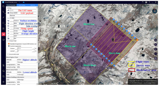
Figure 4.
Flight route planning and parameter statistics from the UAV Butler system (picture shows the route and parameters based on the pre-scanning mission of the fourth block).
The error analysis was based on the reference DSM and a comparison of the various DEM data. The differences between the DEMs and the DSM can easily be calculated from Equation (1), and it could be completed using ArcGIS Pro software:
where represents the errors; and are the elevation data from the free and open-source products and InSAR-derived results from the Sentinel-1a images and the result obtained from the UAV pre-scanning photos. All units were in m.
After the calculation of the errors, all the DEMs and DSM were then used for flight route planning based on the UAV Butler system, and the parameters were recorded, which included the ground surface resolution, flight height, average elevation, highest altitude, and the lowest altitude for each small survey area. The parameters gained from planning based on the DSM were the reference, which were compared with the other statistics from the six DEMs (i.e., ascending InSAR-derived DEM, descending InSAR-derived DEM, and four open-source DEMs). Furthermore, to clearly show the spatial distribution characteristics of the elevation errors, we drew error distribution maps and calculated the normalized error index [34], which can be computed as per Equation (2). Based on the index, it is easy to see the region where the elevation was with the largest difference:
where represents the normalized error index; , and are the error values of each pixel, the maximum value and the minimum value of the error raster data maps obtained from Equation (1), respectively.
According to the planning principle of UAV flight routes, the ground surface resolution, the average elevation, and the highest elevation are considered [62,63]. For the same camera with a higher flight altitude, the ground surface distance (GSD) becomes larger, and the ground surface resolution of the products obtained from UVA images becomes lower [64,65]. Counting the smallest flight altitude of the four black lines, compared with the maximal value of the absolute error obtained from the other DEMs and the DSM, the availability and safety of the DEMs used for UAV flight route planning can be known.
Concretely, in this paper, we took the flight height and acquired surface resolution of the UAV pre-scan mission as the optimal result and also as a comparison criterion, which was used to compare the performances of the route planning based on different DEMs with the same parameters setting in mountainous surroundings. If the ground surface is smaller than the reference (route planning based on the DSM), there may be some dangers in this route planning. On the other hand, the availability and safety depend on the relationship between the maximal absolute error value and the minimal lowest route altitude. Namely, if the maximum absolute value is smaller than the minimum route altitude, this route plan is feasible and safe, with the lower flight altitude the more excellent way.
4. Results and Analysis
4.1. Results of Pre-Scanning Aerial Drone Images
The DSM and orthophoto products with a surface resolution of 0.1 m could be obtained by processing the pre-scanning UAV aerial photos with high-accuracy POS by the Pix4Dmapper. The results are shown in Figure 5.
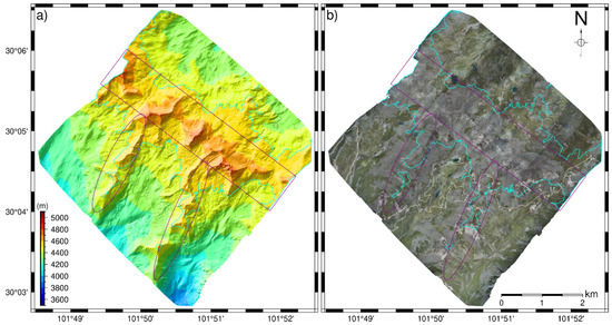
Figure 5.
Pre-scan results of the drone: (a) surface DSM map; (b) orthophoto map. The winding, white line features on the orthophoto map are the roads built for the installation of the transmission line towers. The dark magenta rectangle box is located in the area of the main mountain range, and the two dark magenta ellipses are the areas of the two lower mountains. The polygon area indicated by cyan is the area with an elevation greater than or equal to 4500 m.
From Figure 5, it can be seen that the DSM (Figure 5a) with a surface resolution of 0.1 m obtained by unmanned pre-scanning work can meticulously portray the topographic features of the covered area in great detail, and it can reflect the topographical characteristics of ridges, valleys, and slopes clearly. The statistics shows that the elevation ranges from 3929.24 to 4785.08 m, with an average value of 4426.24 m, and the standard deviation (SD) was 137.29 m, and it was a complex mountainous surrounding. The orthophoto (Figure 5b) shows that the area was mainly covered with gravel stone, less grass, and no trees. Especially at the mountain ridges (dark magenta rectangle box and ellipses in Figure 5), where the elevation was equal to or greater than 4500 m (cyan polygon in Figure 5), breakstones were everywhere, and no vegetation or water bodies existed. The landcover features were coincident with the Google satellite images (Figure 2c, Section 2). In addition, with the natural physicochemical weathering effect, there was a large amount of rubble that had accumulated near the roads (Figure 5b), which needs more attention.
4.2. DEM Acquired by InSAR Processing Based on Sentinel-1 Images
The two DEMs of the study area were obtained from InSAR processing with the ascending and descending SAR images, and the results are shown in Figure 6.
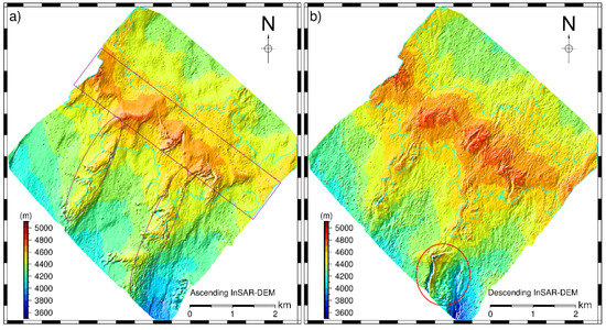
Figure 6.
DEMs obtained from Sentinel-1a InSAR processing: (a) generated from Sentinel-1a ascending data and (b) descending data. The location of the main mountain range is marked by the dark magenta rectangle, the two dark magenta ellipses represent the location of the two lower mountains, and the area inside and outside the irregular-shaped cyan polygon is the area with an elevation greater than or equal to 4500 m. The red circle in (b) indicates the region with large differences in DEM.
The DEMs’ statistics show that the ascending InSAR-derived DEM ranged from 3858.56 to 4827.54 m, with a mean and STD of 4416.50 and 148.70 m, respectively. The descending InSAR-derived DEM varied from 3533.30 to 5018.02 m, and the average and STD were 4460.15 and 161.07 m. Compared with the reference DSM statistics, it can be found that the ascending InSAR-derived DEM was more coincident with the real terrain. In addition, comparing Figure 6 with Figure 5a, it can be found that there were some large and significant errors in the descending InSAR-derived elevation data, not only in the main mountain region (dark magenta rectangle in Figure 5a and Figure 6a) but also in the two lower mountain ranges (the two dark magenta ellipses in Figure 5a and Figure 6a). In detail, the InSAR-derived DEMs data are higher in the high-latitude mountain area (large than 4500 m; namely, the area within the cyan polygon in Figure 5a and 6), while the elevation value in the low-altitude area is lower than the UAV aerial survey results. This phenomenon is more obvious for the DEM data obtained from the descending SAR images. More specifically, there were obvious gully-like details (red circles in Figure 6b) along the mountain direction, which may be caused by the smaller perpendicular baseline and atmospheric effects.
4.3. Errors in the Different DEMs Based on the UAV DSM
The errors and normalized error indexes between the various DEMs and reference DSM were calculated by applying Equations (1) and (2) based on the ArcGIS Pro software platform, and the spatial distribution maps are shown in Figure 7. In addition, the quantitative counting analyzing histograms are shown in Figure 8.

Figure 7.
Errors and normalized error indexes of the DEMs based on the reference DSM: (a–f) correspond to errors in the spatial distribution maps of the ascending InSAR DEM (with a resolution of 13.96 m), descending InSAR DEM (with a resolution of 13.96 m), ALOS PALSAR DEM (with a resolution of 12.5 m), ASTER Global DEM V3 (with a resolution of 30 m), SRTM V3 DEM (with a resolution of 30 m), and TanDEM (with a resolution of 90 m), respectively. On the top left, the scale represents the scaling factor and the range indicates the error value range. The actual error value is the product of scale and index.
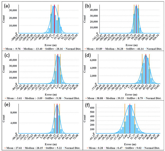
Figure 8.
Statistical histograms of the elevation errors based on the UAV DSM reference: (a–f) correspond to errors in the statistical histograms of the ascending InSAR DEM, descending InSAR DEM, ALOS PALSAR DEM, ASTER Global DEM V3, SRTM V3 DEM, and TanDEM, respectively.
From Figure 7, the absolute elevation difference values of all error maps were within 85 m (Figure 7c–f), except the two InSAR-derived DEMs (Figure 7a,b). The maximum absolute error of the ascending InSAR-derived DEM was near 300 m, while for the descending InSAR-derived data it was greater than 700 m, and all were extremely relevant to the accuracy of the SAR processing. It was obvious that the DEM from the ascending SAR image processing results were best. Through comprehensive analysis of all of the maps, the characteristics of the error distribution were found, specifically, that large differences appeared in the slope bodies of the mountain ranges, while in other locations, the errors were relatively small.
From the error statistical histograms in Figure 8, we can observe the difference between each DEM clearly. The error statistical parameters are also shown for each histogram, including the mean, median, and SD, and all the error distributions conformed to a normal distribution. The elevation means and the corresponding median were very close, and all were within 0.55 m, except the InSAR-derived DEMs (3.64 m for the ascending and 2.39 m for the descending). Combined with the SD values, we found that the open-source DEMs seemed to perform better over the two InSAR-derived DEMs, and the ascending one performed better than the descending DEM.
Furthermore, in combination with Figure 8 and Figure 7, the spatial distribution maps were highly coincident with the histograms. The maximum absolute values of each DEM were 300.19, 742.14, 84.22, 77.94, 72.08, and 61.27 m, respectively, and except for the ASTER DEM, all other DEMs were distributed with negative error values greater than the positive data. The distribution positions of all error data were located more closely to the positive than the negative; that is to say that the extreme outliers of the DEMs may appear in the negative values, which may occur with the outlier from the reference DSM.
4.4. UAV Route Planning Based on Different DEMs/DSM
To analyze the practicability of each DEM applied for flight route planning, all the DEMs imported material into the UAV Butler system for the route plan, and the results of the statistical parameters are shown in Table 3.
Table 3.
Route planning results of the statistical parameters based on the different reference datasets.
As can be observed from Table 3, the parameters of the results obtained from the DSM were the reference for all of the other DEMs. The parameters contained the optimal ground surface resolution (OGSR, m), flight height (FH, m), average elevation (AE, m), highest altitude (HA, m), lowest altitude (LA, m), and the elevation error range (EER, m). For the same load instrument for the UAV, the higher resolution was derived from the lower flight altitude. The maximum elevation of the survey was lower than the absolute flight altitude (average elevation plus the route altitude), which is the essential condition for safe UAV flying. In other words, the maximum absolute of the EER must be smaller than the minimum flight altitude of the four blocks to ensure the UAV survey safety for the whole survey area. Then, when comparing the OGSR, if the OGSR is smaller than the DSM result, there may be some risks for this route plan strategy. If the OGSR is equal to or slightly greater than the DSM result, this route plan strategy performs excellently. If the OGSR is greater than the DSM result, there is no risk for UAV flying, but the products obtained from these mission images were relatively rough.
Comparing and analyzing the statistical parameters in Table 3, the minimum flight altitude of the descending InSAR-derived DEM was 612 m, smaller than the maximum absolute elevation errors at 742.14 m, and this means that this flight plan strategy was unbecoming. For the TanDEM, the OSGR of the second block was smaller than that of the reference UAV DSM, and this means that it may be a risk for this route plan strategy, and it is not suitable for UAV survey tasks in mountainous surroundings. The ascending InSAR-derived DEM applied for UAV route planning in this survey area was practicable, but the resolution of the generated products was rough, ranging from 0.12 to 0.16 m, which performed more roughly than the UAV pre-scanning mission (0.10 m). Among the DEMs, using the SRTM DEM for route plans performed excellently, and the OSGR of each block was equal to the DSM with the smallest elevation errors, ranging from −50.19 to 72.08 m.
5. Discussion
5.1. Factors for the InSAR-Derived DEM Process
From the analysis of the DEMs used for UAV route planning, we found that the ascending InSAR-derived DEM has potential, while the resolution of the aerial survey results was rough. Applying the descending InSAR-derived DEM was not feasible, because there is a crash risk. The main reason for this is the performance of the InSAR-derived DEMs. The DEM data of the survey area can be successfully obtained by InSAR processing of Sentinel-1a images covering the whole aerial area, but they are extremely limited by the perpendicular baseline and temporal baseline of the Sentinel-1a imagery pairs. The ascending pair (perpendicular baseline at 84.54 m and a temporal baseline with 12 days) performed better than the descending pair (perpendicular baseline at 31.87 m and a temporal baseline with 12 days) within the entire area. This is consistent with the findings of Braun [47]. The larger perpendicular baseline was more sensitive to terrain with a consistent temporal baseline; therefore, the ascending data with a larger perpendicular baseline were more sensitive to the terrain and had better results. Especially in the higher elevation parts of the mountains, as shown in Figure 6a, they were obviously more consistent with the actual terrain (comparing Figure 6 with Figure 5a).
InSAR technology was originally proposed for surface topography mapping [37,48], and the high-accuracy DEM data produced by the SRTM mission [33] were the excellent and successful realization of this theory. At present, InSAR technology itself is very dependable, and the differences in the results are very slight, even if some parameters in the processing are adjusted [34,36,46,47]. Although Sentinel-1 data do not have advantages in DEM production due to the limitation of its own band (C-band) for DEM generation, it has a very short revisit interval (12 days for a single star and up to 6 days for the constellation of double stars), which is very attractive [47]. The acquisition of surface DEMs extracted from InSAR technology depends on a smaller temporal baseline and a larger perpendicular baseline of SAR image pairs covering the entire survey area. As for the Sentinel-1 SAR data, they have a great advantage in temporal baseline, but for the perpendicular baseline, there is large randomness.
To decrease the errors induced by the time inconsistency, because of the lack of the Sentinel-1b images, the Sentinel-1a images at the 12 days interval were selected for DEM generation, and the acquisition date was as close to the UAV pre-scanning assignment. The perpendicular baseline was as large as possible. Despite all this, there were some other factors that affected the result’s performance, e.g., the difference in the orbits’ direction, earth flattening effect, atmosphere effect, and other noises [48,56]. All of these will lead to diversities in the wrapped interferograms and coherence graphs generated in the processing (Figure 9), which are useful to justify the reliability of the InSAR processing.
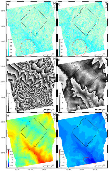
Figure 9.
Related products during the InSAR processing: (a), (c), (e) and (b), (d), (f) are the coherence, interferogram, and unwrapped phase data of the ascending and descending data, respectively. The temporal baseline of both the ascending and descending data is 12 days, and the perpendicular baseline is 84.54 and 31.87 m, respectively. The black polygon is the area surveyed by the UAV, the red circle indicates the points with large differences in coherence, and the red rectangle shows the area with anomalies.
Focusing only on the coherence coefficients, it can be found that the coherence was better in the region where the UAV measurement area was located, in most regions with values greater than 0.6 (Figure 9a,b), and where the decorrelation was not severe. In terms of the whole region, the coherence coefficient maps produced by the descending images were better than the ascending data in many regions (as shown in the red circles in Figure 9a,b). However, for the interferogram with the wrapped phase (Figure 9c,d), the ascending pair was significantly better than the descending one, showing more regular interference fringes. It was also more sensitive to the topographic phase, attributed to the larger perpendicular baseline, accompanied by a better performance between the unwrapped phase and the actual elevation (Figure 9e,f).
The unwrapped phase approach is also a critical parameter in InSAR processing, and the unwrapped method used in this paper was the minimum cost flow (MCF) [57,59,66], with a whole full tile for the unwrapping processing in the Snaphu software due to the small InSAR processing range. It turns out that there was a phase mutation in the south (the red rectangle in Figure 9f), and adjusting the unwrapped parameters did not solve this problem. However, considering that the area was not within the UAV survey area and the subsequent route planning did not refer to these DEM products, the elevation product generated from this data did not have a significant impact on the results, and no further study was conducted. However, if the sudden phase mutation occurs within the ROI, it needs to be focused on and interpreted, otherwise the incorrect results may be introduced into the UAV route plan, which may induce an inadequate strategy.
5.2. InSAR-Derived DEMs for UAV Route Plans
InSAR-derived elevation products are relatively new compared to free and open-source DEMs, and they are attractive and have potential in UAV route planning to replace pre-scanning work. Although the spatial resolution of these InSAR-derived DEMs is rough, with the successful launch of SAR satellites, increasingly, SAR images with higher resolutions are available, which will promote the resolution and ensure the safety of UAV flights based on these elevation products. It is fully feasible and hopeful to understand the characteristics of each SAR dataset amply and to select suitable imageries for DEM generation for application in UAV route planning for aerial survey missions, and this is an alternative to the time-consuming and laborious UAV pre-scanning work.
For the UAV pre-scanning processing, in this paper, we undertook the mission with a visible light camera with an equal flight height. In fact, compared with light detection and ranging (LiDAR) technology [67] or oblique air surveys [55], this approach is not the most optimal strategy for topographic mapping [64,67,68], which may induce errors to the reference DSM itself. However, compared with free and open-source DEMs, the DSM has advantages not only in terms of timeliness but also in spatial resolution, and this ensures that the error analysis based on this DSM is sufficient. If the pre-scanning mission is undertaken with the LiDAR or an oblique air survey method, the reference DSM may be more accurate, but this is not necessary for a pre-scanning mission.
6. Conclusions
In this paper, DEMs with a resolution of 13.96 m covering the UAV pre-scanning survey area were generated from the ascending and descending Sentinel-1a data based on InSAR processing of the complex Zheduoshan Mountains. These two DEMs were used for UAV route planning to verify the practicability, which is hoped to replace the time-consuming and laborious UAV pre-scanning work. At the same time, four other free and open-source DEM products were also used in the route plans, calculating the elevation errors based on the reference DSM to analyze the practicability of this strategy. The conclusions obtained are as follows:
- (1)
- For UAV surveys in mountainous regions, pre-scanning missions can provide an accurate DSM to plan routes for lower flight heights to obtain higher-resolution images, but it is time consuming and laborious.
- (2)
- Of the UAV route plans based on the four free and open-source DEMs, the SRTM DEM with a spatial resolution of 30 m performed the best, with an elevation error ranging from −50.19–72.08 m. The ASTER GDEM performed second best, while the TanDEM, at a resolution of 90 m, is not recommended.
- (3)
- Elevation products generated from Sentinel-1 images based on InSAR technology with a larger perpendicular baseline are a useful approach for complex mountains that are treeless. The DEMs can depict the terrain relatively well, and a good consistency exists according to the reference DSM, which is potentially valuable for UAV route plans.
- (4)
- Time-consuming and labor-intensive pre-scanning missions will hopefully be replaced with the easy InSAR-derived DEMs or existing precise DEMs, which can improve field UAV aerial survey efficiency and decrease the waste of time.
Author Contributions
Conceptualization, Q.D. and G.L.; methodology, Q.D. and G.L.; software, Q.D.; validation, Q.D., G.L., Y.Z., D.C., and S.Q.; formal analysis, Q.D., M.C., and Y.C.; investigation, Q.D. and Y.Z.; resources, G.L.; data curation, Q.D. and G.L.; writing—original draft preparation, Q.D. and G.L.; writing—review and editing, Q.D. and G.L.; visualization, Q.D.; supervision, D.C., Y.Z., M.C., Y.C., S.Q., L.T., and H.J.; project administration, G.L., D.C., Y.C., L.T., and H.J.; funding acquisition, G.L. and D.C. All authors have read and agreed to the published version of the manuscript.
Funding
This research was funded by the Second Tibetan Plateau Scientific Expedition and Research Program (Grant No. 2019QZKK0905), the National Natural Science Foundation of China (Grant No. U1703244), the Foundation of the State Key Laboratory of Frozen Soil Engineering (Grant No. SKLFSE-ZY-20), and the Foundation of the State Key Laboratory for Geomechanics and Deep Underground Engineering (Grant No. SKLGDUEK 1904).
Data Availability Statement
The DSM and Orthophoto dataset of the survey area can be downloaded from the National Tibetan Plateau Data Center(http://data.tpdc.ac.cn/en/ (accessed on 8 September 2022)). Other relevant data and GMT codes can be obtained by contacting the corresponding author.
Acknowledgments
Thanks to the ESA (https://scihub.copernicus.eu/dhus/#/home (accessed on 1 July 2022)), Earth Data (https://search.earthdata.nasa.gov/search (accessed on 1 July 2022)), ASF (https://search.asf.alaska.edu (accessed on 1 July 2022)), and OGC (https://geoservice.dlr.de/web (accessed on 1 July 2022)) organizations or institutions for providing free and open-source datasets to support this paper. We thank the anonymous reviewers for their insightful and constructive comments on this manuscript, and we also thank the editor and associate editor for their invaluable help with our manuscript.
Conflicts of Interest
The authors declare no conflict of interest.
References
- Jiang, J.; Johansen, K.; Tu, Y.-H.; McCabe, M.F. Multi-Sensor and Multi-Platform Consistency and Interoperability between UAV, Planet CubeSat, Sentinel-2, and Landsat Reflectance Data. GIsci. Remote Sens. 2022, 59, 936–958. [Google Scholar] [CrossRef]
- Bhardwaj, A.; Sam, L.; Martín-Torres, F.J.; Kumar, R. UAVs as Remote Sensing Platform in Glaciology: Present Applications and Future Prospects. Remote Sens. Environ. 2016, 175, 196–204. [Google Scholar] [CrossRef]
- Colomina, I.; Molina, P. Unmanned Aerial Systems for Photogrammetry and Remote Sensing: A Review. ISPRS J. Photogramm. Remote Sens. 2014, 92, 79–97. [Google Scholar] [CrossRef]
- Yu, J. Quadrotor Unmanned Aerial Vehicle Design and Realization. Master Thesis, South China University of Technology, Guangzhou, China, 2018. [Google Scholar]
- Zhang, Y. Research on the Low-Altitude Safety from the Perspective of Risk Regulation: Take the Civil Unmanned Aerial Vehicle Management and Control in Beijing as an Example. Master Thesis, People’s Public Security University of China, Beijing, China, 2020. [Google Scholar]
- Sun, Z.; Wang, X.; Wang, Z.; Yang, L.; Xie, Y.; Huang, Y. UAVs as Remote Sensing Platforms in Plant Ecology: Review of Applications and Challenges. J. Plant Ecol. 2021, 14, 1003–1023. [Google Scholar] [CrossRef]
- Karl, J.W.; Yelich, J.V.; Ellison, M.J.; Lauritzen, D. Estimates of Willow (Salix Spp.) Canopy Volume Using Unmanned Aerial Systems. Rangel Ecol. Manag. 2020, 73, 531–537. [Google Scholar] [CrossRef]
- Getzin, S.; Wiegand, K.; Schöning, I. Assessing Biodiversity in Forests Using Very High-Resolution Images and Unmanned Aerial Vehicles. Methods Ecol. Evol. 2012, 3, 397–404. [Google Scholar] [CrossRef]
- Chisholm, R.A.; Cui, J.; Lum, S.K.Y.; Chen, B.M. Uav Lidar for Below-Canopy Forest Surveys. J. Unmanned Veh. Syst. 2013, 1, 61–68. [Google Scholar] [CrossRef]
- Tziavou, O.; Pytharouli, S.; Souter, J. Unmanned Aerial Vehicle (UAV) Based Mapping in Engineering Geological Surveys: Considerations for Optimum Results. Eng. Geol. 2018, 232, 12–21. [Google Scholar] [CrossRef]
- Messina, G.; Modica, G. Applications of UAV Thermal Imagery in Precision Agriculture: State of the Art and Future Research Outlook. Remote Sens. 2020, 12, 1491. [Google Scholar] [CrossRef]
- Rokhmana, C.A. The Potential of UAV-Based Remote Sensing for Supporting Precision Agriculture in Indonesia. Procedia Environ. Sci. 2015, 24, 245–253. [Google Scholar] [CrossRef]
- Giordan, D.; Adams, M.S.; Aicardi, I.; Alicandro, M.; Allasia, P.; Baldo, M.; de Berardinis, P.; Dominici, D.; Godone, D.; Hobbs, P.; et al. The Use of Unmanned Aerial Vehicles (UAVs) for Engineering Geology Applications. Bull. Eng. Geol. Environ. 2020, 79, 3437–3481. [Google Scholar] [CrossRef]
- Forster, M.C.A. Implications of Climate Change for Hazardous Ground Conditions in the UK. Geol. Today 2004, 20, 61–67. [Google Scholar] [CrossRef]
- Valkaniotis, S.; Papathanassiou, G.; Ganas, A. Mapping an Earthquake-Induced Landslide Based on UAV Imagery; Case Study of the 2015 Okeanos Landslide, Lefkada, Greece. Eng. Geol. 2018, 245, 141–152. [Google Scholar] [CrossRef]
- Giordan, D.; Hayakawa, Y.; Nex, F.; Remondino, F.; Tarolli, P. Review Article: The Use of Remotely Piloted Aircraft Systems (RPASs) for Natural Hazards Monitoring and Management. Nat. Hazards Earth Syst. Sci. 2018, 18, 1079–1096. [Google Scholar] [CrossRef]
- Bolognesi, M.; Farina, G.; Alvisi, S.; Franchini, M.; Pellegrinelli, A.; Russo, P. Measurement of Surface Velocity in Open Channels Using a Lightweight Remotely Piloted Aircraft System. Geomat. Nat. Hazards Risk 2017, 8, 73–86. [Google Scholar] [CrossRef]
- Stöcker, C.; Bennett, R.; Nex, F.; Gerke, M.; Zevenbergen, J. Review of the Current State of UAV Regulations. Remote Sens. 2017, 9, 459. [Google Scholar] [CrossRef]
- Aasen, H.; Honkavaara, E.; Lucieer, A.; Zarco-Tejada, P.J. Quantitative Remote Sensing at Ultra-High Resolution with UAV Spectroscopy: A Review of Sensor Technology, Measurement Procedures, and Data Correctionworkflows. Remote Sens. 2018, 10, 1091. [Google Scholar] [CrossRef]
- Katrašnik, J.; Pernuš, F.; Likar, B. A Survey of Mobile Robots for Distribution Power Line Inspection. IEEE Trans. Power Deliv. 2010, 25, 485–493. [Google Scholar] [CrossRef]
- Yuan, Z. Research on Application of UAV in Transmission Line Engineering Construction. In Proceedings of the 2021 International Conference on Machine Learning and Intelligent Systems Engineering, MLISE, Chongqing, China, 9–11 July 2021; pp. 420–424. [Google Scholar] [CrossRef]
- Li, X.; Li, Z.; Wang, H.; Li, W. Unmanned Aerial Vehicle for Transmission Line Inspection: Status, Standardization, and Perspectives. Front. Energy Res. 2021, 9, 336. [Google Scholar] [CrossRef]
- Gangolu, S.; Sarangi, S. A Novel Complex Current Ratio-Based Technique for Transmission Line Protection. Prot. Control Mod. Power Syst. 2020, 5, 1–9. [Google Scholar] [CrossRef]
- la Scalea, R.; Rodrigues, M.; Osorio, D.P.M.; Lima, C.H.; Souza, R.D.; Alves, H.; Branco, K.C. Opportunities for Autonomous UAV in Harsh Environments. In Proceedings of the 16th International Symposium on Wireless Communication Systems, Oulu, Finland, 27–30 August 2019; pp. 227–232. [Google Scholar] [CrossRef]
- Fahrner, W.R.; Job, R.; Werner, M. Sensors and Smart Electronics in Harsh Environment Applications. Microsyst. Technol. 2001, 7, 138–144. [Google Scholar] [CrossRef]
- Gitardi, D.; Giardini, M.; Valente, A. Autonomous Robotic Platform for Inspection and Repairing Operations in Harsh Environments. Int. J. Comput. Integr. Manuf. 2021, 34, 666–684. [Google Scholar] [CrossRef]
- Wong, C.; Yang, E.; Yan, X.-T.; Gu, D. Autonomous Robots for Harsh Environments: A Holistic Overview of Current Solutions and Ongoing Challenges. Syst. Sci. Control. Eng. 2018, 6, 213–219. [Google Scholar] [CrossRef]
- Mazzini, F.; Dubowsky, S. An Experimental Validation of Robotic Tactile Mapping in Harsh Environments Such as Deep Sea Oil Well Sites. Springer Tracts Adv. Robot. 2014, 79, 557–570. [Google Scholar] [CrossRef]
- Valavanis, K.P.; Vachtsevanos, G.J. Handbook of Unmanned Aerial Vehicles; Springer: Berlin/Heidelberg, Germany, 2015; pp. 1–3022. [Google Scholar] [CrossRef]
- Granshaw, S.I. Photogrammetric Terminology, 4th ed.; John Wiley & Sons, Ltd: Hoboken, NJ, USA, 2020; Volume 35. [Google Scholar]
- Du, Q.; Li, G.; Li, J.; Zhou, Y. Research on the River Extraction Based on the DEM Data in the Central West Tianshan Mountains. China Rural Water Hydropower 2020, 10, 29–33, 40. [Google Scholar] [CrossRef]
- Yao, B.; Zhou, W. Research on Hydrological Characteristics Extraction of Chanba Basin Based on DEM and ArcGIS. J. Water Resour. Water 2017, 28, 8–13. [Google Scholar] [CrossRef]
- Dewitt, J.D.; Warner, T.A.; Conley, J.F. Comparison of DEMS Derived from USGS DLG, SRTM, a Statewide Photogrammetry Program, ASTER GDEM and LiDAR: Implications for Change Detection. GIsci. Remote Sens. 2015, 52, 179–197. [Google Scholar] [CrossRef]
- Qingsong, D.; Guoyu, L.; Wanlin, P.; Yu, Z.; Mingtang, C.; Jinming, L. Acquiring High-Precision DEM in High Altitude and Cold Area Using InSAR Technology. Bull. Surv. Mapp. 2021, 3, 44–49. [Google Scholar] [CrossRef]
- Mejías, L.; Correa, J.F.; Mondragón, I.; Campoy, P. COLIBRI: A Vision-Guided UAV for Surveillance and Visual Inspection. In Proceedings of the 2007 IEEE International Conference on Robotics and Automation, Roma, Italy, 10–14 April 2007; pp. 2760–2761. [Google Scholar] [CrossRef]
- Zhou, H.; Zhang, J.; Gong, L.; Shang, X. Comparison and Validation of Different DEM Data Derived from InSAR. Procedia Environ. Sci. 2012, 12, 590–597. [Google Scholar] [CrossRef][Green Version]
- Graham, L.C. Synthetic Interferometer Radar for Topographic Mapping. Proceeding IEEE 1974, 62, 763–768. [Google Scholar] [CrossRef]
- Chaabani, A.; Deffontaines, B. Application of the SBAS-DInSAR Technique for Deformation Monitoring in Tunis City and Mornag Plain. Geomat. Nat. Hazards Risk 2020, 11, 1346–1377. [Google Scholar] [CrossRef]
- Imamoglu, M.; Kahraman, F.; Cakir, Z.; Sanli, F.B. Ground Deformation Analysis of Bolvadin (W. Turkey) by Means of Multi-Temporal InSAR Techniques and Sentinel-1 Data. Remote Sens. 2019, 11, 1069. [Google Scholar] [CrossRef]
- Zhou, Y.; Stein, A.; Molenaar, M. Integrating Interferometric SAR Data with Levelling Measurements of Land Subsidence Using Geostatistics. Int, J. Remote Sens. 2003, 24, 3547–3563. [Google Scholar] [CrossRef]
- JIA, S.; ZHANG, T.; FAN, C.; LIU, L.; SHAO, W. Research Progress of InSAR Technology in Permafrost. Adv. Earth Sci. 2021, 36, 694. [Google Scholar] [CrossRef]
- Kimura, Y.Y.H. Detection of Landslide Areas Using Satellite Radar Interferometry. Photogramm Eng. Remote Sens. 2000, 66, 337–344. [Google Scholar]
- Li, X.; Zhou, L.; Su, F.; Wu, W. Application of InSAR Technology in Landslide Hazard: Progress and Prospects. Yaogan Xuebao/Natl. Remote Sens. 2021, 25, 614–629. [Google Scholar] [CrossRef]
- Lu, Z.; Dzurisin, D. InSAR Imaging of Aleutian Volcanoes; Springer: Berlin/Heidelberg, Germany, 2014. [Google Scholar] [CrossRef]
- Garthwaite, M.C.; Miller, V.L.; Saunders, S.; Parks, M.M.; Hu, G.; Parker, A.L. A Simplified Approach to Operational InSAR Monitoring of Volcano Deformation in Low-and Middle-Income Countries: Case Study of Rabaul Caldera, Papua New Guinea. Front Earth Sci. (Lausanne) 2019, 6, 240. [Google Scholar] [CrossRef]
- Wegmüller, U.; Santoro, M.; Werner, C.; Strozzi, T.; Wiesmann, A.; Lengert, W. DEM Generation Using ERS–ENVISAT Interferometry. J. Appl. Geophys. 2009, 69, 51–58. [Google Scholar] [CrossRef]
- Braun, A. Retrieval of Digital Elevation Models from Sentinel-1 Radar Data—Open Applications, Techniques, and Limitations. Open Geosci. 2021, 13, 532–569. [Google Scholar] [CrossRef]
- Zebker, H.A.; Goldstein, R.M. Topographic Mapping from Interferometer SAR Observations. J. Geophys. Res. 1986, 91, 4993–5000. [Google Scholar] [CrossRef]
- Liu, Y.; Gong, Y.; Li, Y.; Zhu, D.; Liu, H.; Shuai, W. Soil Stoichiometric Characteristics of Alpine Shrub Meadowat Different Elevations, Western Sichuan. J. Sichuan Agric. Univ. 2018, 36, 167–174. [Google Scholar] [CrossRef]
- Wang, X. GIS-Based Study on Temperature Lapse Rate in Mountain Areas in China. Master Thesis, Nanjing University of Information Science & Technology, Nanjing, China, 2015. [Google Scholar]
- Yang, Y. Study on Freeze-Thaw Damage Mechanism of Different Lithologic Rocks with Fractures. Master Thesis, Chengdu University Of Technology, Chengdu, China, 2018. [Google Scholar]
- Zhou, T.; NARAYAN, P.G.; LIAO, L.; Zhang, L.; Wang, J.; Sun, J.; Wei, Y.; Xie, Y.; Wu, Y. Spatio-Temporal Dynamics of Two Alpine Treeline Ecotones and Ecological Characteristics of Their Dominate Species at the Eastern Margin of Qinghai-Xizang Plateau. Chin. J. Plant Ecol. 2018, 42, 1082–1093. [Google Scholar] [CrossRef]
- Xiang, Q.; Pan, J.; Zhang, G.; Xu, Z.; Zhang, D.; Tu, W. Monitoring and Analysis of Surface Deformation in the Zheduoshan Area of Sichuan-Tibet Railway Based on SBAS Technology. Eng. Surv. Mapp. 2020, 48–54+59. [Google Scholar] [CrossRef]
- Shan, J.; Li, Z.; Zhang, W. Recent Progress in Large-Scale 3D City Modeling. Acta Geod. Et Cartogr. Sin. 2019, 48, 1523–1541. [Google Scholar] [CrossRef]
- Nex, F.; Remondino, F. UAV for 3D Mapping Applications: A Review. Appl. Geomat. 2013, 6, 1–15. [Google Scholar] [CrossRef]
- Shan, X.J.; Ye, H. The INSAR Technique: Its Principle and Applications to Mapping the Deformation Field of Earthquakes. Acta Seismol. Sin. 1998, 11, 759–769. [Google Scholar] [CrossRef]
- Yu, H.; Lan, Y.; Yuan, Z.; Xu, J.; Lee, H. Phase Unwrapping in InSAR: A Review. IEEE Geosci Remote Sens. Mag. 2019, 7, 40–58. [Google Scholar] [CrossRef]
- SNAPHU. Available online: https://web.stanford.edu/group/radar/softwareandlinks/sw/snaphu/ (accessed on 5 July 2022).
- Chen, C.W.; Zebker, H.A. Network Approaches to Two-Dimensional Phase Unwrapping: Intractability and Two New Algorithms. JOSA A 2000, 17, 401–414. [Google Scholar] [CrossRef]
- Chen, C.W.; Zebker, H.A. Two-Dimensional Phase Unwrapping with Use of Statistical Models for Cost Functions in Nonlinear Optimization. J. Opt. Soc. Am. A Opt. Image Sci. Vis. 2001, 18, 338. [Google Scholar] [CrossRef]
- Chen, C.W.; Zebker, H.A. Phase Unwrapping for Large SAR Interferograms: Statistical Segmentation and Generalized Network Models. IEEE Trans. Geosci. Remote Sens. 2002, 40, 1709–1719. [Google Scholar] [CrossRef]
- Chai, M.; Li, G.; Ma, W.; Chen, D.; Du, Q.; Zhou, Y.; Qi, S.; Tang, L.; Jia, H. Damage Characteristics of the Qinghai-Tibet Highway in Permafrost Regions Based on UAV Imagery. Int. J. Pavement Eng. 2022, 1–12. [Google Scholar] [CrossRef]
- Valavanis, K.P.; Vachtsevanos, G.J. UAV Design Principles: Introduction. In Handbook of Unmanned Aerial Vehicles; Springer: Berlin/Heidelberg, Germany, 2015; pp. 107–108. [Google Scholar] [CrossRef]
- Müller, J.A.; Ehlers, T.; Gollnick, V. Drone Routing Optimizer for Aerial Inspections of Energy and Railway Infrastructures. In Proceedings of the AIAA AVIATION 2022 Forum, Chicago, IL, USA, 27 June–1 July 2022. [Google Scholar] [CrossRef]
- Dermanis, A. The Photogrammetric Inner Constraints. ISPRS J. Photogramm Remote Sens. 1994, 49, 25–39. [Google Scholar] [CrossRef]
- Zhang, B.; Li, J.; Ren, H. Using Phase Unwrapping Methods to Apply D-InSAR in Mining Areas. Can. J. Remote Sens. 2019, 45, 225–233. [Google Scholar] [CrossRef]
- Guan, H.; Sun, X.; Su, Y.; Hu, T.; Wang, H.; Wang, H.; Peng, C.; Guo, Q. UAV-Lidar Aids Automatic Intelligent Powerline Inspection. Int. J. Electr. Power Energy Syst. 2021, 130, 106987. [Google Scholar] [CrossRef]
- Hu, Z.-L.; Deng, Y.-Z.; Peng, H.; Han, J.-M.; Zhu, X.-B.; Zhao, D.-D.; Wang, H.; Zhang, J. Optimal Path Planning with Minimum Inspection Teams and Balanced Working Hours For Power Line Inspection. Front Phys. 2022, 10, 657. [Google Scholar] [CrossRef]


Publisher’s Note: MDPI stays neutral with regard to jurisdictional claims in published maps and institutional affiliations. |
© 2022 by the authors. Licensee MDPI, Basel, Switzerland. This article is an open access article distributed under the terms and conditions of the Creative Commons Attribution (CC BY) license (https://creativecommons.org/licenses/by/4.0/).