A Novel Waveform Decomposition and Spectral Extraction Method for 101-Channel Hyperspectral LiDAR

Abstract

The 101-channel full-waveform hyperspectral LiDAR (FWHSL) is able to simultaneously obtain geometric and spectral information of the target, and it is widely applied in 3D point cloud terrain generation and classification, vegetation detection, automatic driving, and other fields. Currently, most waveform data processing methods are mainly aimed at single or several wavelengths. Hidden components are revealed mainly through optimization algorithms and comparisons of neighbor distance in different wavelengths. The same target may be misjudged as different ones when dealing with 101 channels. However, using the gain decomposition method with dozens of wavelengths will change the spectral intensity and affect the classification. In this paper, for hundred-channel FWHSL data, we propose a method that can detect and re-decompose the channels with outliers by checking neighbor distances and selecting specific wavelengths to compose a characteristic spectrum by performing PCA and clustering on the decomposition results for object identification. The experimental results show that compared with the conventional single channel waveform decomposition method, the average accuracy is increased by 20.1%, the average relative error of adjacent target distance is reduced from 0.1253 to 0.0037, and the degree of distance dispersion is reduced by 95.36%. The extracted spectrum can effectively characterize and distinguish the target and contains commonly used wavelengths that make up the vegetation index (e.g., 670 nm, 784 nm, etc.).

1. Introduction

Full-waveform light detection and ranging (FW-LiDAR) is a new remote sensing detection technology developed from traditional LiDAR [1]. Compared with discrete LiDAR systems, full-waveform LiDAR can record complete signals [2,3] and characterize the interaction process of transmitter pulses with the surface of an object [4,5]. Given these advantages, full-waveform LiDAR has been increasingly used in surface topography exploration, land cover classification [6,7,8], vegetation structure, physiological detection [9,10,11], 3D urban terrain modeling [12], and many other remote sensing applications.

Developed from FW-LiDAR, full-waveform hyperspectral LiDAR (FWHSL) can obtain the target’s distance, spectrum, and other information simultaneously by virtue of the supercontinuum laser source (SCL) and high-sensitivity detection technology. FWHSL can record both transmitter and echo waveform data of the target in multiple channels in a short time, which dramatically improves the ability to obtain vertical spectra and biochemical distributions for vegetation and land cover classification [13,14,15]. In 2012, the Finnish Geospatial Research Institute (FGI) developed a 16-channel HSL system, which successfully collected three-dimensional point clouds with spectral information from vegetation samples and extracted chlorophyll and water content parameters [16,17]. Subsequently, FGI realized a tunable HSL system with the use of an acousto-optic tunable filter (AOTF) [18], which achieved backscattered echo with continuous coverage of the full spectrum of 500–1000 nm.

However, due to the development of detection technology and more complex detection scenes and requirements, some problems have arisen in the study of HSL detection results [12,14,19]. For example, under different channels and incident angles, the response of the target’s surface to the laser beams will vary, which can result in extremely low-intensity echo signals of the target being recorded in some channels. In contrast, a target component with high intensity may obscure the previous target’s echo, leading to the waveform components being missed in the decomposition results [12,20]. Due to the group velocity dispersion and non-linear effects [21,22] caused by the SCL and various light speeds at multiple laser wavelengths in the same transmission medium, the target may be identified as two false targets with different center positions in different channels. As a result of the “sub-footprint” effect, when a laser foot is irradiated on the edge of one target, the waveform component’s intensity parameters for all targets may be significantly reduced in some channels. Spectra consisting of intensity information from each channel will be quite different from those in normal conditions, which will affect the measurement of target-related vegetation indicators and the acquisition and discrimination of spectra [23,24]. In summary, the negative factors mentioned above will lead to incorrect decomposition results and the retrieval of unrealistic waveform components and parameters (e.g., intensity, center position, pulse width, etc.), which will eventually affect the extraction of distance and spectrum information of the occluded target [25].

Some scholars have proposed reasonable solutions to the problems described above. For instance, the radar equation combined with the improved bi-directional reflection distribution function (BRDF) model is used to correct the low-intensity results caused by incident angle and scanning range [26,27]; the interference of soft-response targets can be eliminated by setting a threshold [23]; and the normalized reflection factor can be used to improve echo intensity caused by the “sub-footprint” effect [24]. However, all of these methods are aimed at correcting the results after data processing and ignore the inner information hidden in LiDAR data during data processing. In order to dig deeply into data processing, Wagner, Neuenschwander, and others applied the decomposition and deconvolution method, which characterizes waveforms by mathematical models such as Gaussian distribution to obtain the target’s detail parameters [28,29,30,31,32]. However, these studies mainly focused on a single wavelength, which can be easily limited by insufficient intensity, leading to the loss of weakly responsive target waveform components [20]. Song first proposed a multispectral waveform decomposition method to search for the hidden waveform components in multiple wavelengths, and help other wavelengths append them [20]. Although the minimum decomposable distance was increased, the method was designed for several channels, and one target could be considered as two when faced with HSL (101-channel) data. Wang found a multi-channel interconnected compensation method to gain the signal’s SNR and reveal hidden components, which was an effective cure for the weakly responsive target echoes due to the “sub-footprint” effect [14], but it also changed the original intensity, which may affect the accuracy of the restored spectrum.

In this study, to solve the problems of both hidden components and distorted spectra, we considered the advantage of the HSL channel number and explored the waveform data in 101 channels, proposing a more straightforward and operational method to deal with 101-channel HSL waveform data; this includes single-channel waveform decomposition (SCWD) and multi-channel mutual complementary decomposition (MCMCD), and a channel selection method to restore the target’s characteristic spectrum. The method can detect and help re-decompose the channels with outliers, by checking neighbor distances and selecting specific wavelengths to compose characteristic spectra based on PCA and clustering for object identification. Furthermore, we designed an HSL detection experiment with the aim of verifying the method’s validity and exploring the spectral changes before and after the target is covered. Our research objectives were as follows:

• To put forward a new decomposition method for HSL waveform data with 101 channels, including SCWD and MCMCD, which will help effectively extract target distance and intensity information in different channels of wavelengths;
• To restore and retrieve the feature spectrum of the target by selecting the wavelength based on the result of assessing HSL decomposition;
• To design an experiment to verify the correctness and effectiveness of this method and explore the spectral changes before and after the target is covered.

2. Materials and Methods

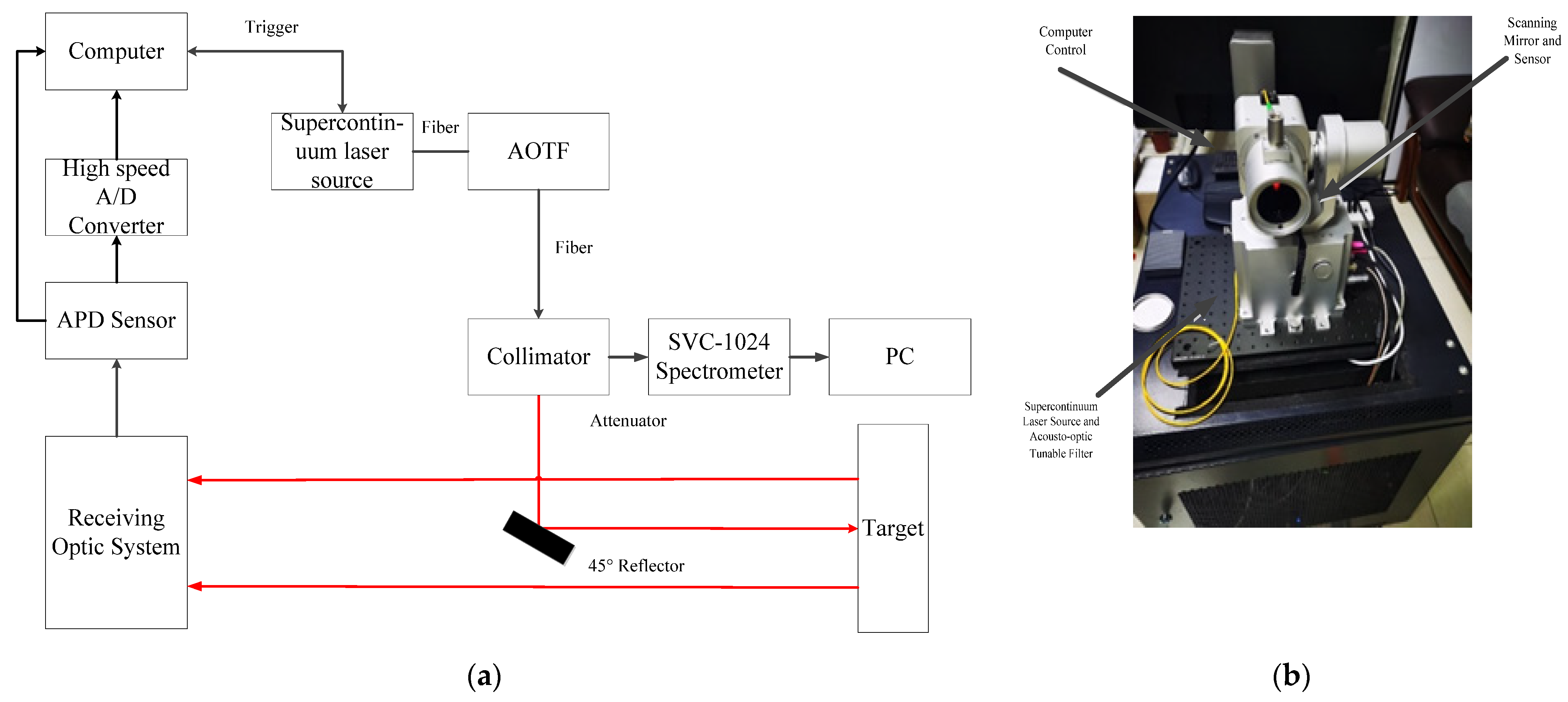
2.1. 101-Channel FWHSL System

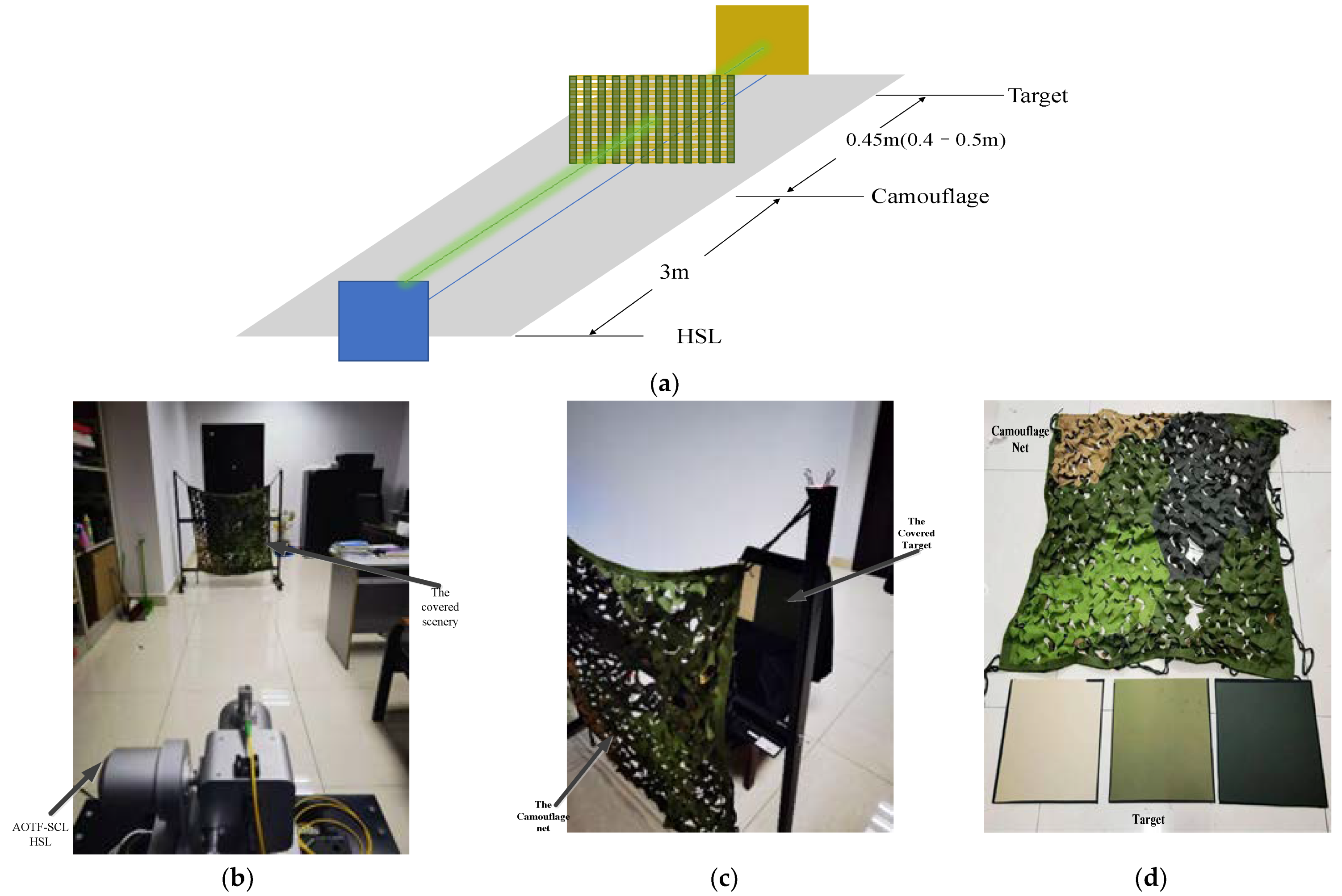
The FWHSL system was developed by Chen at FGI [18] and other scholars [33]. Schematic and physical diagrams of the hyperspectral full-waveform LiDAR system are shown in Figure 1a,b. The overall system adopts a Ritchey–Chretien (R-C) structure, which is usually composed of a primary and secondary mirror and a primary and secondary correction mirror. It is also composed of an SCL, an AOTF, a 2-dimensional scanning turntable, a coaxial transmitter–receiver system, a multi-channel full-waveform detection unit, and a host computer.

The AOTF is a tunable narrow band-pass filter with bandwidths ranging from a few to tens of nanometers that exploits acousto-optic effects to diffract and shift the frequency of light. In the proposed system, due to the high tuning speed of the AOTF, it only takes half a millisecond to obtain the full spectrum in the current full spectrum configuration when the AOTF device is synchronized with the broadband laser source [18]. Thus, the laser transmitter unit composed of AOTF and SCL achieves continuous spectral wavelength selection and generates laser signals sequentially with different wavelengths in the same period. Then the laser is collimated and expanded by a fiber coupling to a reflective collimator, and finally is incident on the target via a 45° reflector.

Calibration of the effect of laser energy emission is achieved by passing a sample of the transmitted signal through the receiver and monitoring the signal (using an SVC-1024 spectrometer and PC) from the standard targets [18]. Furthermore, a white (whole band) reflectance standard board with 99% reflectivity is measured 5 times to verify its energy stability. It can be seen that the spectra of the white reflectance standard board are always in a stable range, which proves that the laser energy is stable during the experiment. In addition, the power spectra of the SCL can be inferred from the test results.

In the experiment, the SCL in the system ranged from 450 to 2400 nm with a maximum power of more than 8 μJ, while the mono-pulse energy in different wavelengths differed, as shown in Figure 2, and the working band of the system was from 550 to 1050 nm. The pulse repetition rate was 500 kHz in average, the full width at half maximum was 2–4 ns, and the spectral resolution was 5 nm; other parameters and indexes are shown in

Table 1. System design criteria of HSL and waveform parameters.

Parameter	Value
Spectral range	550–1050 nm
Spectral resolution	5 nm (101 channels)
Co-efficiency of AOTF crystal diffraction	>80%
Output efficiency	>40%
Polarization	Line polarization
Mono-pulse energy	>8 μJ
Divergence angle of light spot	~0.35 mrad
Collimator focal length	33 mm
Sampling rate	5 GHz/s
FWHM	2–4 ns

. Generally, the product of diffraction efficiency, optical aperture, spectral resolution, and solid angle is defined as the “co-efficiency” of the AOTF, indicating that the energy loss of the “white laser” after AOTF splitting is small. The scattered laser pulses were collected by a Cassegrain telescope (with 700 mm focal length and 100 mm aperture diameter). The focal point of the telescope is imaged onto a high-voltage-biased low-noise-level avalanche photodiode (APD) model [18] consisting of a silicon APD and an integrated amplifier with a bandwidth of 1 GHz, which converts the laser echo into an electronic signal and amplifies it, effectively suppressing the noise. After testing, the system could obtain hyperspectral waveform data at 37.5 m with random error [18]. The system was installed with a high-speed acquisition card (sampling rate 5 GS/s) for sampling and storage, which can simultaneously record the waveform of the transmitter pulse and the received echo.

2.2. Experiment

The purpose of the experiment was to carry out basic scientific exploration, with the hope that the results could be widely used in various shading scenarios, such as reconnaissance of camouflaged targets, canopy vegetation surveys, etc., so an experiment with a universal shading scene including covered object detection was designed without the pertinence of the scene. The presence of multiple targets can lead to the acquisition of overlapping waveform data, and the proposed method can be used for waveform decomposition. Moreover, the rich spectral information obtained by processing hyperspectral waveform data can be used to distinguish targets and delimit the same target region, which will be convenient for subsequent point cloud expansion and identification.

To test the applicability and accuracy of the proposed method in obtaining the distance and spectrum information of covered targets, we designed a 2-step experiment. The first step was to construct an experimental scenario in which the LiDAR transmits the camouflage net to irradiate the covered target. We placed the HSL, the camouflage net, and the target plate on the experimental platform along the same axis direction. The distance between the HSL and the camouflage net was 3 m, and the distance between the camouflage net and the target was 0.45 m. The schematic and actual scenes of the scenario are shown in Figure 3a–c, and experimental equipment is shown in Figure 3c. The 3 target boards in Figure 3c are targets to be measured whose spectral properties are unknown, used for different experimental purposes. They are not the standard reflector boards used to calibrate spectra. In this experiment, only the leftmost target board was used as the target covered by the camouflage net. Next, we removed the camouflage net while keeping the other experimental conditions unchanged. HSL scanned the above scenes to collect the waveform data of 101 wavelength channels.

2.3. Methods

The echoes in various receiving channels can differ significantly due to the irregular energy distribution of SCL [14], different target sensitivity to multiple wavelengths, and various types of interference during signal transmission, propagation, and reception [34]. Moreover, when dealing with 101 channels, the method of finding the difference in distance between two adjacent components as a new component in the multispectral LiDAR waveform decomposition method is more complicated, and it is easy to mistake the same target for two different targets. To overcome these disadvantages and improve operability, we propose an HSL data processing method for 101 channels to extract accurate parameters and select feature channels in a 4-step flow, as shown in Figure 4. First, valid channel selection and synchronous calibration of the time domain are performed for the transmitter and echo pulses in each channel as a preprocessing step. Then, the skew normal distribution (SND) function is used to perform single-channel waveform decomposition for each channel, including denoising and filtering, for estimation and optimization of parameters. Third, the difference in distance between two adjacent targets is set as a judgment index to detect hidden components and channels with wrong decomposition results, which will be re-decomposed. Finally, indexes including intensity, pulse width, center position, and evaluation in the decomposition result are chosen, and principal component analysis is performed to select a specific group of channel wavelengths to form the characteristic spectrum through clustering. The method includes valid channel selection and synchronous calibration of the time domain, 101-channel waveform decomposition, and spectrum restoration.

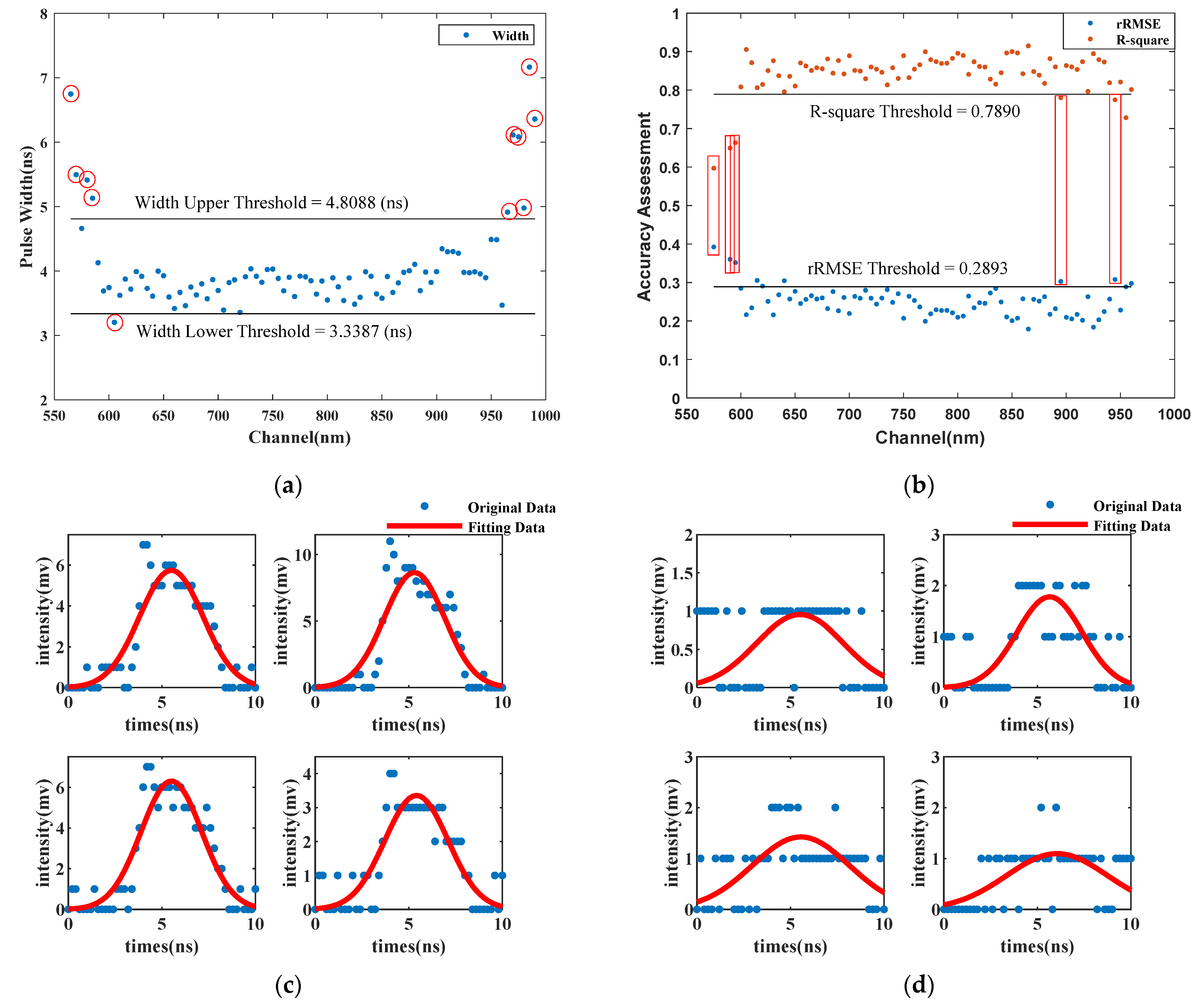
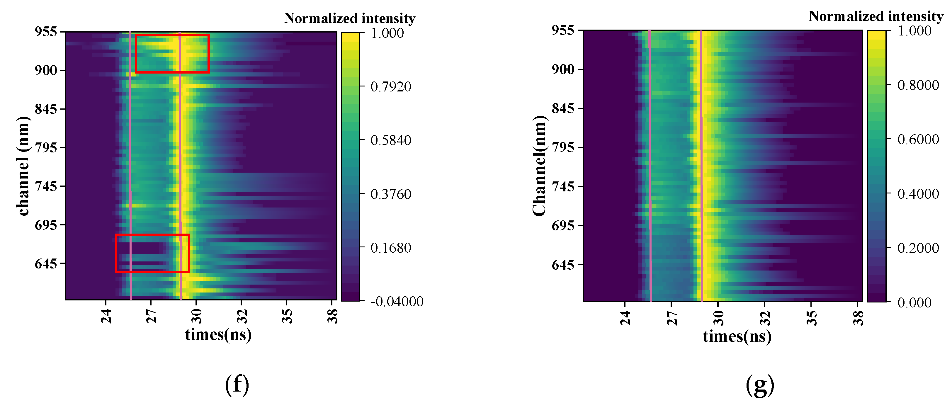
2.3.1. Valid Channel Selection and Synchronous Calibration of Time Domain

Due to the irregular energy distribution of SCL and other factors, such as sampling error, the results of waveforms recorded in some channels will be inferior and make no contribution to the retrieval of target distance and spectrum information. Therefore, it is necessary to select the channels with useful information recorded during the preprocessing step.

The channel selection process is divided into two steps. The first step is to eliminate all channels with a maximum intensity value of less than 4 mv, because the signals recorded by those channels are too weak to extract useful information. The second step is to eliminate the channels with poor recording of the transmission waveform, as those channels cannot determine the center position of the transmission pulse as the starting point, and it makes no sense to determine the actual distance of the target by the center position of the echo.

The second step was designed as two-step process. First, we fit the transmission pulses of the remaining channels after the first elimination step with the Gaussian distribution model to obtain the parameter of pulse width (FWHM) $F_{{\lambda }_j,trans}$ and the accuracy evaluation indexes for the fitting results of each channel, including root mean square error (RMSE), relative RMSE (rRMSE), and coefficient of determination (R²). Then we counted the mean value of the center time ${\overline{s}}_{trans}$, the mean value and standard deviation of the pulse width, and the evaluation indexes of all channels (${\overline{F}}_{trans}$, ${\delta }_{F_{{\lambda }_j}}$, $rRMS{E}_{mean}$, $R^2{}_{mean}$, $rRMS{E}_{std}$, and $R^2{}_{std}$). The first threshold ($th{r}_{pw}$) was set between the average plus or minus the standard deviation (${\overline{F}}_{{\lambda }_j,trans} \pm {\delta }_{F_{{\lambda }_j}}$) of the pulse width. The second and third threshold values ($th{r}_{rRMSE}$ and $th{r}_{R^2}$) were set as the average of rRMSE plus its standard deviation ($rRMS{E}_{mean}+rRMS{E}_{std}$) and the average of R² minus its standard deviation ($R^2{}_{mean}-R^2{}_{std}$). Channels with an FWHM value of the transmitter pulse that is not within the range of the first threshold will be discarded first, and then channels with an rRMSE value more than $th{r}_{rRMSE}$ and R² less than $th{r}_{R^2}$ will also be scrapped. These three thresholds will eliminate poorly recorded channels caused by inevitable factors, which cannot recover the starting time by fitting the transmission pulse.

The Gaussian distribution model, parameters, and evaluation index for the transmitter pulse are described as follows:

$$f_{{\lambda }_j,trans}(t)=A_{{\lambda }_j,trans}\exp (-\frac{{(t-s_{{\lambda }_j,trans})}^2}{F_{{\lambda }_j,trans}^2/(4\ln 2)}), (j=1,2\dots n)$$

(1)

$${\overline{s}}_{trans}=\frac{{\displaystyle \sum _{j=1}^n{s}_{{\lambda }_j,trans}}}{n}$$

(2)

$${\overline{F}}_{trans}=\frac{{\displaystyle \sum _{j=1}^n{F}_{{\lambda }_j,trans}}}{n}$$

(3)

$$RMS{E}_{{\lambda }_j}=\sqrt{\frac{1}{n}{\displaystyle \sum _{j=1}^n(y_j-f_{{\lambda }_j,trans}(t))}}$$

(4)

$$rRMS{E}_{{\lambda }_j}=\frac{RMS{E}_{{\lambda }_j}}{{\overline{y}}_{\lambda }}$$

(5)

$$R_{{\lambda }_j}^2=1-\frac{{\displaystyle \sum _{j=1}^n{(y_j-f_{{\lambda }_j,trans}(t))}^2}}{{\displaystyle \sum _{j=1}^n{(y_j-{\overline{y}}_{\lambda })}^2}}$$

(6)

where $f_{{\lambda }_j,trans}(t)$ denotes the modeled waveform as a function of time t at the jth channel; $A_{{\lambda }_j,trans}$, $s_{{\lambda }_j,trans}$, and $F_{{\lambda }_j,trans}$ represent the waveform parameters of intensity, center location, and FWHM, respectively, for the transmit pulse at the jth channel; $y_j$ and ${\overline{y}}_{\lambda }$ represent the originally recorded waveform data and its average value in the order given at the jth channel; and n is the total number of channels.

Since the time of data recording by each channel is not synchronized due to the HSL system characteristics [25], the step of synchronous calibration in the time domain for each channel is essential to avoid taking the same target as two new targets. After removing the channels with inadequate fitting and defective recording, we measured the average value of the center position of the transmitted pulse of each remaining channel as the unified starting point ${\overline{s}}_{trans}$, and shifted the data of each channel in the appropriate time domain by calculating the difference between the center position at the jth channel and the average (Equation (7)).

$$\mathsf{\Delta }{t}_j=s_{{\lambda }_j,trans}-{\overline{s}}_{trans}$$

(7)

where $\mathsf{\Delta }{t}_j$ denotes the time shift at the jth channel. If $\mathsf{\Delta }{t}_j<0$, the center position should shift right, and vice versa.

2.3.2. 101-Channel HSL Waveform Decomposition Method

• Denoising and Filtering

Before filtering and decomposition, we estimated the noise level from the beginning and ending parts of the echo data as stable background noise without an active signal [20]. We calculated the mean value (Equation (8)) and standard deviation (Equation (9)) of the noise to estimate its level and set the noise threshold ${\delta }_{thr}$ as the mean value plus three times the standard deviation (Equation (10)) to distinguish the signal from the noise:

$${\mu }_{j,noise}=\frac{{\displaystyle \sum _{i=1}^k{n}_{i_{begin,end}}}}{k}$$

(8)

$${\sigma }_{j,noise}=\sqrt{\frac{{\displaystyle \sum _{i=1}^k{(n_{i_{beginning,ending}}-{\mu }_{j,noise})}^2}}{k}}$$

(9)

$${\delta }_{thr}={\mu }_{j,noise}+3{\sigma }_{j,noise}$$

(10)

where $n_{i_{begin,end}}$ represents the value of the beginning and ending parts of the echo data at the jth channel, $k$ is the amount of echo data, and ${\mu }_{j,noise}$ and ${\sigma }_{j,noise}$ represent the mean value and standard deviation of the noise, respectively.

Some studies have compared the effects of Gaussian, Savitzky–Golay, and wavelet filtering on HSL data [25]. They found that wavelet filtering performs best; it not only effectively retains the details of the echo data but also eliminates the influence of noise to the maximum extent, while Gaussian and Savitzky–Golay filtering are not as effective. Thus, we smoothed and denoised the echo data with a Bayesian level 2 bior6.8 wavelet filter and soft threshold. The filtering was done using the Wavelet Signal Denoiser app in MATLAB (2021), set up with the corresponding options.

• Modeling

Single-channel waveform decomposition involves selecting the fitting model, estimating and optimizing the initial parameters of the components, and performing an accuracy assessment of the decomposition result. Traditionally, Gaussian functions have been used to fit full-waveform echoes [35], but the distribution of the waveform may be more asymmetrical due to the uncertainty in the process of transporting and receiving. It was found that the skew normal distribution (SND) model is a better alternative to the Gaussian model, because it can solve the asymmetry problem of the waveform by choosing an appropriate skew coefficient, which not only retains the assumption of Gaussian distribution but also fits the asymmetric echo waveform [32]. Moreover, when the skew coefficient equals zero, the SND model is transformed into a Gaussian model. Thus, we adopted the SND model (Equation (11)) for waveform decomposition:

$$f_{{\lambda }_j,echo}(t|A_i,s_i,{\alpha }_i,F_i)={\displaystyle \sum _{i=1}^m{A}_i·\exp [-\frac{{(t-s_i)}^2}{F_i{}^2/(4\ln 2)}][1+erf({\alpha }_i\frac{t-s_i}{F_i/2\sqrt{\ln 2}})]}$$

(11)

where $f_{{\lambda }_j,echo}(t|A_i,s_i,{\alpha }_i,F_i)$ denotes the modeled waveform as a function of time t at the jth channel and is the superposition of $m$ SND functions, which stands for the echo waveform components; $A_i,s_i,F_i$ represent the intensity, center position, and FWMH, respectively, of the ith waveform component at the jth channel; ${\alpha }_i$ represents the skew coefficient of the SND model; $A_i$ stands for the key value in composing the target’s spectrum; $s_i$ is essential for retrieving distance information; and erf denotes the error function [32].

• Single-Channel Waveform Decomposition (SCWD) Step

The initial parameter estimation process includes a layer-stripping strategy and a seeker optimization algorithm (SOA). Compared with the traditional method of searching for inflection points, the layer-stripping strategy is less affected after denoising and filtering and can obtain relatively ideal and accurate initial parameters. The process of the strategy can be summarized as follows: Seek the data of the maximum current waveform and its position as the strength and center of the waveform parameters, and then determine the FWHM by looking for the half-peak position. Generate the initial parameter set for the SND model and minimize it from the original waveform data, then seek another set until the maximum value is less than the noise threshold.

Since there remains a difference between the actual data and the SND model, whose parameters are replaced with the initial estimated values by the layer-stripping strategy, we used the SOA for further iteration and fitting to obtain a more accurate group of parameters. The SOA uses a combination of random and prior knowledge to treat the waveform components as the population of the problem. One part of the population is generated completely randomly, and the other part is changed within a small range based on the initial value of the waveform component obtained by layer stripping. Then the two parts are combined into the same population, and RMSE is used as the objective function to calculate the value of each waveform component in turn and evaluate its advantages and disadvantages. There is corresponding mature code in MATLAB to realize the SOA.

Given that the objective reality conditions can constrain specific parameters such as FWHM and are allowed to set the limitation range of the value in TR optimization [32], TR was selected rather than Levenberg–Marquardt (LM) as the optimization method. TR optimization is a numerical method for solving nonlinear optimization problems, starting from the given initial values, through stepwise iteration and continuous improvement, until a satisfactory approximate optimal solution is obtained. The basic idea is to transform the optimization problem into a series of simple local optimization problems. We can set the corresponding options to perform TR optimization in MATLAB. Therefore, we performed TR optimization on the estimated components at each channel using the SND model, limiting the FWHM range to between 0.5 and 2 times the known objective pulse width and setting the amplitude greater than the noise threshold. The obtained parameters are the decomposition results for the ith waveform component at the jth channel; the maximum value of i is the number of decomposed waveform components.

For the final obtained waveform components, we used RMSE, rRMSE, and R² to evaluate the decomposition accuracy for every single channel in SCWD. By replacing the parameters of the SND model with optimized values, those assessment indexes were calculated as in Equations (4)–(6).

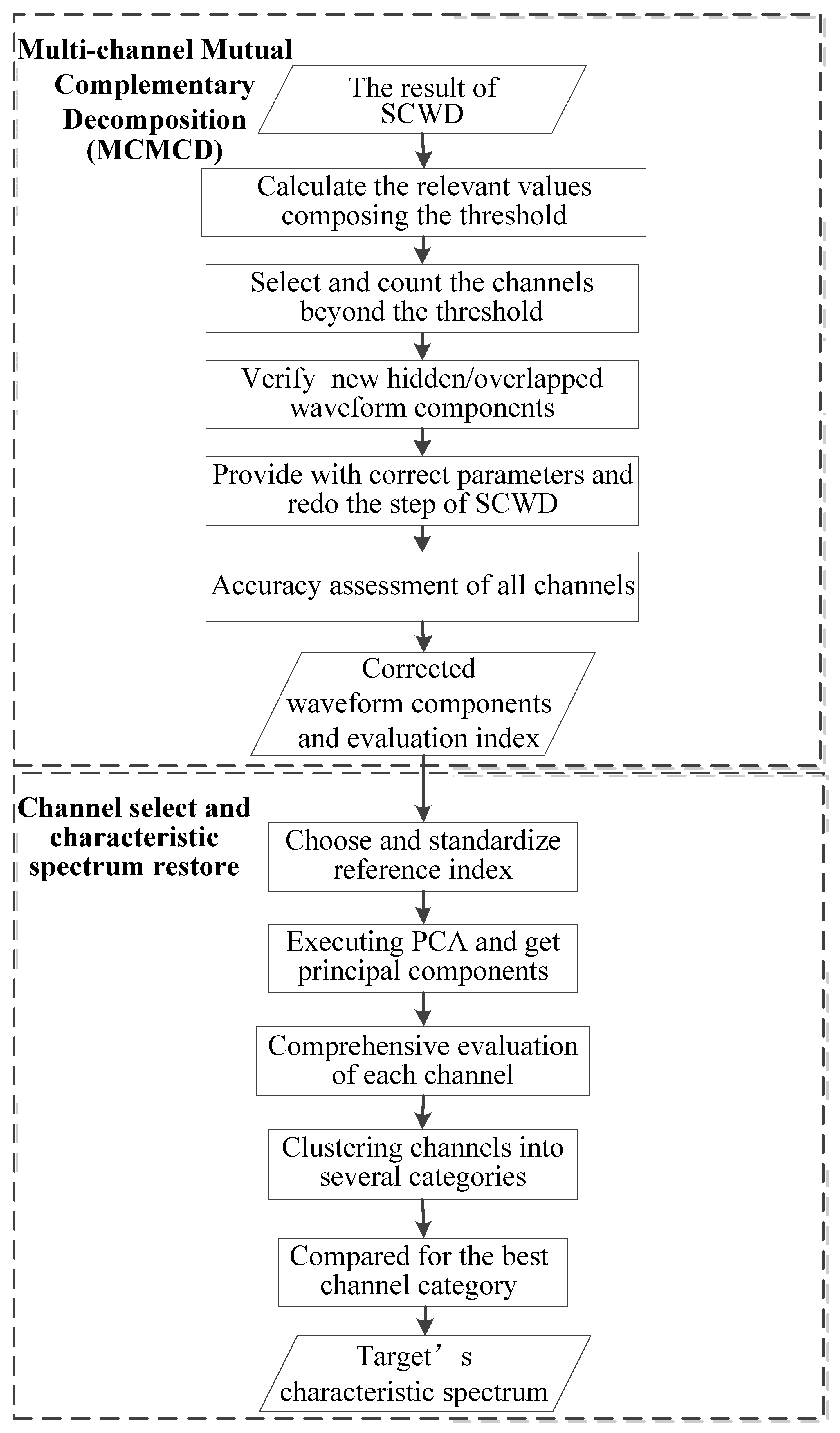
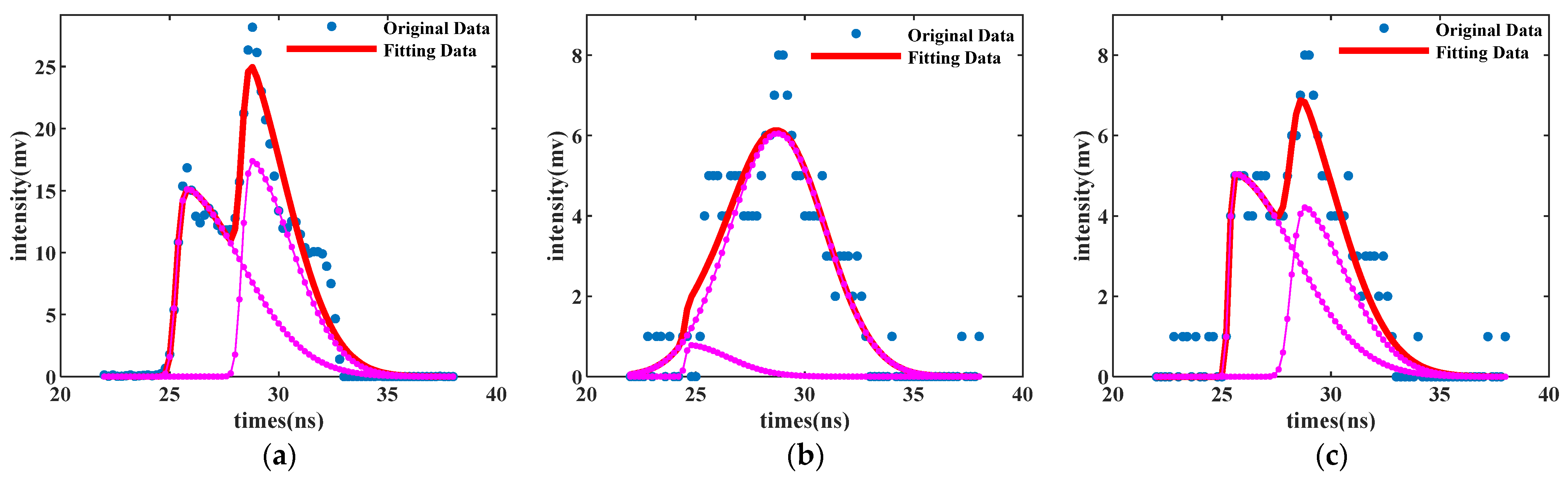
• Multi-Channel Mutual Complementary Decomposition (MCMCD) Step

A significant advantage of AOTF-HSL is the ultra-wide detectable spectral range (550–1050 nm, 101 channels) and high spectral resolution (5 nm), which suggests that most targets will respond strongly to the laser signal in a particular band of the spectrum corresponding to specific channels of the HSL. Given the advantage of a large number of HSL channels, to avoid missing components caused by a weak response of the target to the laser at a particular channel wavelength, we should select the channel with appropriate decomposition results to assist other channels with erroneous outcomes to decompose again and reveal the hidden waveform component.

For the result obtained by SCWD, we counted the difference between the center position of two adjacent sub-echo waveform components $\mathsf{\Delta }{s}_{{\lambda }_j,i}$ in all channels (Equation (12)) and set the threshold $th{r}_{\mathsf{\Delta }s}$ as the average of the difference ${\overline{s}}_i$ plus or minus its standard deviation ${\sigma }_{\mathsf{\Delta }{s}_i}$ (Equations (13)–(15)). Suppose the difference in distance at the jth channel far exceeds the average and is not within the threshold. This suggests that there exist remaining waveform components that are not revealed, or the result of SCWD at the jth channel may be false.

$$\mathsf{\Delta }{s}_{{\lambda }_j,i}=s_{{\lambda }_j,i+1}-s_{{\lambda }_j,i}$$

(12)

$${\overline{s}}_i=\frac{{\displaystyle \sum _{j=1}^n\mathsf{\Delta }{s}_{{\lambda }_j,i}}}{n}$$

(13)

$${\sigma }_{\mathsf{\Delta }{s}_i}=\sqrt{\frac{{\displaystyle \sum _{j=1}^n{(\mathsf{\Delta }{s}_{{\lambda }_j,i}-{\overline{s}}_i)}^2}}{n}}$$

(14)

$$th{r}_{\mathsf{\Delta }s}={\overline{s}}_i\pm {\sigma }_{\mathsf{\Delta }{s}_i}$$

(15)

The differences in specific channels not within the threshold will be considered outliers, indicating that the corresponding channel should be re-decomposed. SND components, including the FWHM and center position parameters, are taken from the channels within the threshold, and the average values are calculated as the initial supplementary parameters for the incorrect channels. Suppose the percentage of outliers is more than 10%. In that case, the position parameter, as the minuend, will be regarded as a newly revealed waveform component, which will be initialized and appended into all other channels for TR optimization. The initial component set comprises the average values for these channels related to the outliers. Furthermore, these channels should also be re-decomposed since they are missing the other waveform components revealed in other channels, whose initial parameters are provided by other correct channels. Suppose the percentage of outliers is less than 10%. In that case, the channels related to the outliers are incorrectly decomposed and should be provided with the correct parameters from other proper channels and re-decomposed. The new parameter set is calculated as pseudo-code according to Equation (16):

$$\begin{array}{l}\mathrm{The} \mathrm{number} \mathrm{of} \mathrm{outliers} \mathrm{is} \mathrm{set} \mathrm{as} “\mathrm{a}”;\\ \mathrm{The} \mathrm{number} \mathrm{of} \mathrm{total} \mathrm{channels} \mathrm{is} \mathrm{set} \mathrm{as} “\mathrm{n}”;\\ if \mathrm{number}(\mathrm{outlier} \mathrm{channels})/\mathrm{number}(\mathrm{total} \mathrm{channels}) \ge 10\%,\\ \mathrm{a} \mathrm{new} \mathrm{component} \mathrm{initial} \mathrm{set}:\{\begin{array}{l}{F}_{new,{\lambda }_j}=\frac{{\displaystyle \sum _{i=1}^a{F}_{{\lambda }_a}}}{a}\\ s_{new,{\lambda }_j}=\frac{{\displaystyle \sum _{i=1}^a{s}_{{\lambda }_a}}}{a}\\ \\ A_{new,{\lambda }_j}=y_{{\lambda }_j}(s_{new,{\lambda }_j})\end{array}\\ elseif \mathrm{number}(\mathrm{outlier} \mathrm{channels})/\mathrm{number}(\mathrm{total} \mathrm{channels}) < 10\%,\\ \mathrm{the} \mathrm{correct} \mathrm{component} \mathrm{set}:\{\begin{array}{l}{F}_{{\lambda }_i}=\frac{{\displaystyle \sum _{j=1}^{n-a}{F}_{{\lambda }_j}}}{n-a}\\ s_{{\lambda }_j}=\frac{{\displaystyle \sum _{j=1}^{n-a}{s}_{{\lambda }_j}}}{n-a}\\ \\ A_{{\lambda }_j}=y_{{\lambda }_j}(s_{{\lambda }_j})\end{array}\end{array}$$

(16)

where $y_{{\lambda }_j}$ is the intensity at time t related to $s_{{\lambda }_j}$ at the jth channel.

By providing the incorrect channels with corrected initial parameters and circulating the re-decomposition until no obvious outliers are found, the distance difference in all channels will be in a stable and reasonable range. As a result, the center positions of the components are taken from each channel, and their average value for each target is finally considered as the measured distance.

After performing the MCMCD step, we re-evaluated the fitting accuracy of the decomposition result for each channel using Equations (4)–(6). However, these indexes only assess single channels; they are irrelevant when determining the accuracy of the distance information measured by overall HSL channels. Therefore, given the advantage of the number of channels, we propose two new assessment indexes, relative error of overall average distance of multiple channels (REOA) and improvement of distance dispersion (IOD), to evaluate the progress of the ranging error and the reduction degree of outliers. REOA and IOD are calculated as Equations (17) and (18):

$$REOA=\frac{\left|\overline{s_i}-s_{real}\right|}{s_{real}}$$

(17)

$$IOD=\frac{{\sigma }_{s_{i,MCMCD}}-{\sigma }_{s_{i,SCWD}}}{{\sigma }_{s_{i,SCWD}}}$$

(18)

where $\overline{s_i}$ and $s_{real}$ represent the measured average distance and actual distance of all channels, respectively, and ${\sigma }_{s_{i,SCWD}}$ and ${\sigma }_{s_{i,MCMCD}}$ are the standard deviation of the ith target after SCWD and MCMCD.

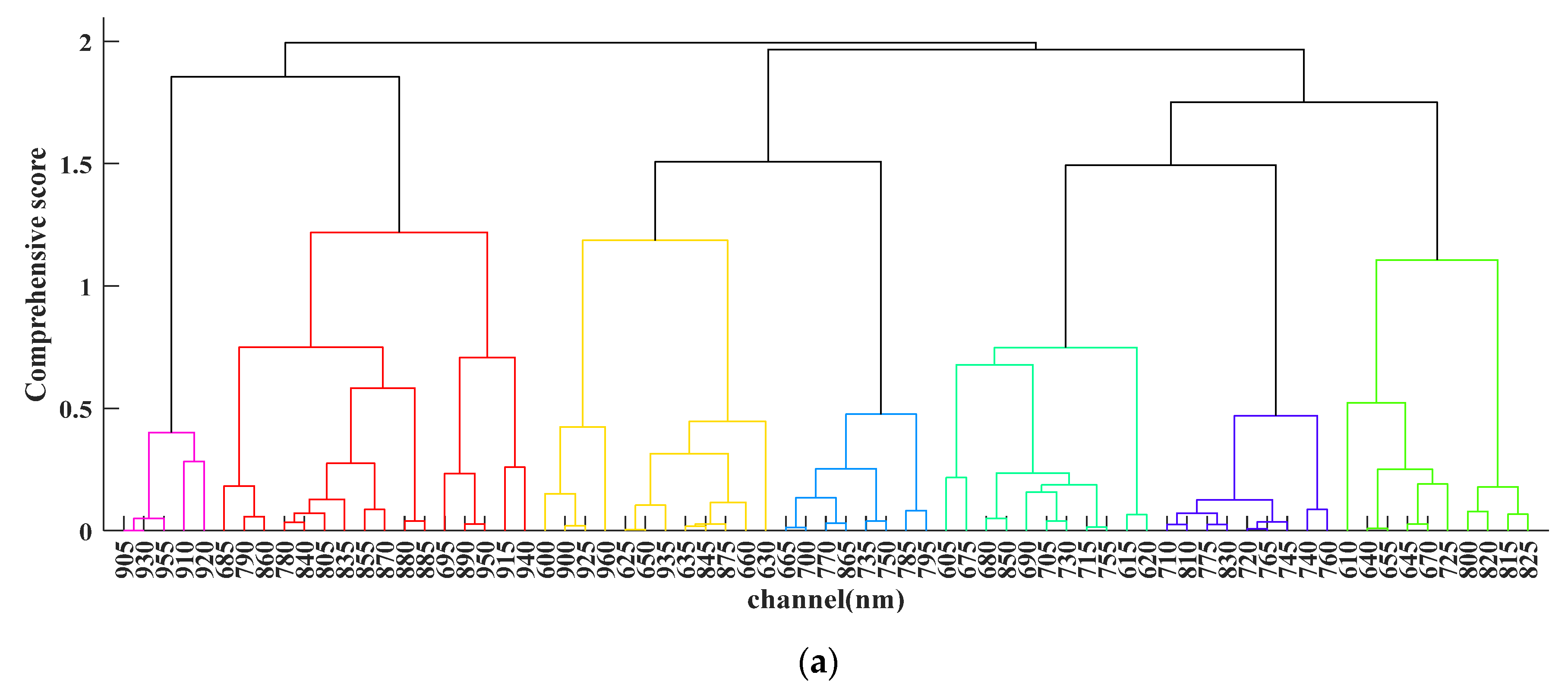
2.3.3. Channel Selection and Spectrum Restoration

Due to the “sub-footprint” effect, the spectrum of the covered object consists of the intensity in all channels, which may differ enormously from that of the uncovered object. Given that many studies have calculated the vegetation index [36] by utilizing different spectra for further exploration, we believe that some representative channels can be selected to constitute the relative spectrum to characterize and distinguish targets, and we propose a channel wavelength selection and relative spectrum restoration method.

These channels can be evaluated by using the information according to the final results of the waveform decomposition. We believe that there is a certain relationship in the parameters (indicators), including position, intensity, FWHM, skew coefficient of the SND model, and accuracy assessment results, in every waveform component, and there are some related parts between them. Using all of these indicators to evaluate the channels will result in ineffective and repeated utilization of some information. Therefore, PCA and dimension reduction can be carried out on these indicators. The new principal components, which can represent more than 93% of the original information [37], can be used to evaluate each channel’s wavelength, and the most representative channels can be selected to form the target’s characteristic spectrum.

First, we chose all of the waveform component parameters and assessment indexes for a single channel as the initial PCA indicators, including intensity, center position, FWHM, skew coefficient, RMSE, rRMSE, and R². The PCA process can be divided into 4 steps:

• Standardize the initial indicators;
• Calculate the covariance matrix of the data and the eigenvalues and eigenvectors of the covariance matrix;
• Sort the eigenvalues from largest to smallest;
• Calculate the contribution rate and select the first several eigenvalues and corresponding eigenvectors whose contribution rate sum can summarize the most original data information;
• Transform the data into a new space constructed from the first several eigenvectors.

The number of samples is set to the number of channels, n, and there are p indicators describing these samples. The contribution rate of the qth principal component (Equation (19)) and the cumulative contribution rate of the previous q principal components (Equation (20)) are then calculated. Some studies have shown that if the cumulative contribution rate exceeds about 93%, it can be considered that the corresponding q previous principal components will include most of the information of all indicators and are not related [37]. Thus, we selected the first q principal components with a total contribution of more than 93% as a comprehensive variable to evaluate the ability of each channel to represent the target.

$$Contributio{n}_q=\frac{{\lambda }_q}{{\displaystyle \sum _{i=1}^p{\lambda }_i}}$$

(19)

$$Contributio{n}_{{\displaystyle \sum q}}=\frac{{\displaystyle \sum _{i=1}^q{\lambda }_i}}{{\displaystyle \sum _{i=1}^p{\lambda }_i}}$$

(20)

Next, we comprehensively evaluated the samples (channels) by the first q principal components selected: first, the distance vectors between pieces were calculated by using a correlation coefficient, and then they were classified according to the principle of maximum distance, and clustering results were obtained. These steps can be performed in MATLAB with corresponding codes. Since the number of HSL channels was large and the evaluation results were correspondingly large, we divided these results by applying the cluster function. The channels were divided into 2, 3, …, n categories, and the first category in each division was chosen to form a characteristic spectrum, as they were the channels with the highest scores.

In the end, we compared the characteristic spectra and selected the one that could effectively distinguish targets as the final characteristic spectrum; the corresponding classification and its first class of channels were regarded as the best-performing channels to represent the target spectrum.

3. Results

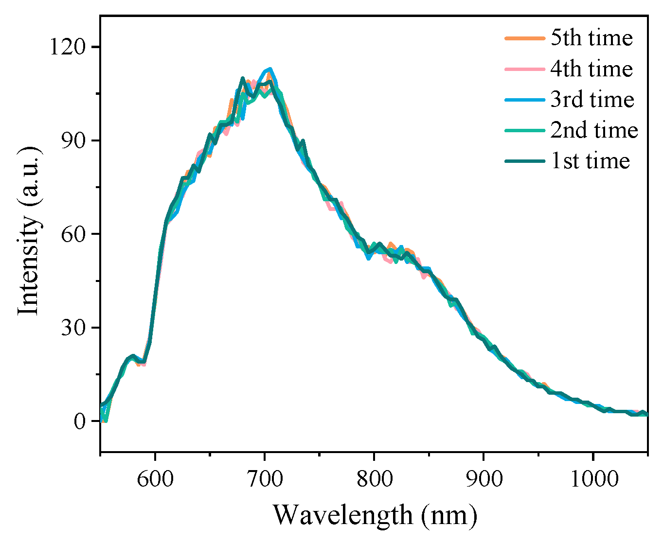
3.1. Valid Channel Selection Results and Calibration of Data in Time Domain

According to the initial channel selection method described in Section 2.3.1, we eliminated the channels with intensity maxima of less than 4 mv, fitted the transmitter pulses of the remaining channels, counted their pulse widths and the fitting accuracy assessment indexes, calculated the mean values and standard deviations, and set the thresholds to continue eliminating worthless channels. The threshold value of pulse width was 3.34–4.81 ns, and all channels not within this interval were picked out; they are marked with red circles in Figure 5a. The channels above the threshold limit of 0.2893 ns for the relative error and below the limit of 0.7890 ns for the correlation coefficient are marked with red rectangles in Figure 5b. Some marked channels’ fitting results (565, 570, 970, and 990 nm) are shown in Figure 5c. It can be observed that these fitting results do not appropriately fit the actual data; all of them have problems, including extremely low intensity (<2 mv) and wide width (>4 ns). In fact, the discrete data recorded in these channels inherently have the problems of inaccurate recording and low intensity; thus, they cannot reasonably reveal the center location of the transmitter pulse or determine the starting time, leading to an inability to determine the final distance of the target. Figure 5d shows some well-fitted channels in the threshold range. The data recorded in these channels differ significantly from those in Figure 5c. Therefore, the channels in Figure 5a,b marked as having poor recording results were eliminated during data preprocessing to avoid interfering with the subsequent retrieval of distance information.

Table 2. Comparison of initial channel selection results considering transmitter pulses.

	Channels		Range of ${\overline{F}}_{trans}$ (ns)		Range of rRMSE		Range of R2
	Before	After	Before	After	Before	After	Before	After
Laser footprint	101	71	4.07 ± 0.74	3.83 ± 0.25	0.26 ± 0.06	0.24 ± 0.03	0.81 ± 0.12	0.85 ± 0.03

shows the changes in the number of channels before and after channel selection, and in the mean value of pulse width, rRMSE, and R², and their standard deviations. There were 101 channels in the beginning, and 70 channels met the requirements after elimination, accounting for 70.3%. The discarded channels were generally poorly recorded, including irregular data and low intensity. The average transmitter pulse width of each channel was reduced from 3.33–4.81 ns to 3.58–4.08 ns, closer to the standard pulse width parameter of 4 ns; the average and maximum values of rRMSE were reduced from 0.26 to 0.24 and from 0.32 to 0.27, respectively; the fitting correlation coefficient R² also improved (≥0.85). This indicates that the channels that were worthless for retrieving target distance and spectral information were successfully eliminated by the threshold restriction, while the channels with better-recorded data were retained.

After eliminating the worthless channels, the mean value of the center position of the transmitted pulses in each channel is calculated as t = 5.3392 ns. It can be seen that the center positions of all channel pulses before correction are scattered around the mean line, as shown in Figure 6a. The statistics of the maximum offset of each channel from the mean value are listed in

Table 3. Starting position of each channel and maximum offset.

	Starting Position (ns)	Left Maximum Offset		Right Maximum Offset
		Time (ns)	Distance (cm)	Time (ns)	Distance (cm)
Laser footprint	5.3392	0.3134	4.7009	0.2383	3.5748

; the difference between the leftmost and rightmost offsets is 0.55 ns, which converted into actual distance is 8.25 cm. Suppose the starting point of the transmitting time is not unified. In that case, the waveform components of the same target may be mistaken as two targets in the subsequent waveform decomposition, which would affect the determination of the number of the targets and the distance information. Therefore, the mean value of the center position (t = 5.3392 ns) is taken as the starting point of the transmitted pulse in each channel, and the data of all channels are shifted in the time domain to the starting point. The calibration result is shown in Figure 6d.

3.2. Distance Retrieval Results and Comparison between SCWD and MCMCD

After performing SCWD and MCMCD in turn, we calculated the distance difference between the two neighbor waveform components in each channel and compared the results of waveform decomposition, as shown in Figure 7. Figure 7a shows the distance difference in all channels and the threshold (upper threshold = 4.1958 ns; lower threshold = 1.0524 ns), and the apparent outliers are marked. It can be seen that the decomposition results of the channels corresponding to 600, 635, 665, 920, and 930 nm, and some others, are problematic. The number of outliers of the same type does not exceed 10%, indicating that no waveform component remained unrevealed. The original data of the 635, 665, 920, and 930 nm channels were compared with the fitting results, as shown in Figure 7b–e. False waveform components were extracted in the 635 nm and 665 nm channels, and the fitting result is not close to the measured data (Figure 7b,c). Moreover, the second waveform component was not revealed for the incorrect initial parameters or mistake optimization in SCWD (Figure 7d,e).

The marked channels should be provided with new initial parameter sets to correct the erroneous decomposition results. Figure 7a also shows that the mistaken channels are surrounded by channels with appropriate decomposition results, suggesting that the mean value of the correct components can be set as supplementary initial parameters for those channels. Therefore, we carried out MCMCD by applying these new initial parameter sets; the results of the distance difference are shown in Figure 7f. Compared to Figure 7a, the distance difference between the two neighbor targets in each channel is in a stable range of 2.67–3.33 ns (corresponding to an actual distance difference in the field of 0.4–0.5 m, with a fluctuation of no more than ±4 cm), which is consistent with the experimental scenario. The 960 nm channel is circled separately because it still deviates too far from the average value after being decomposed by MCMCD. The channel’s data are no longer used when retrieving the target distance information, due to its abnormal recordings.

The new decomposition results of all channels after MCMCD are shown in Figure 7g–j; compared with Figure 7b–f, the fitting accuracy was improved intuitively. The mistake of the false component was corrected (Figure 7g,h); the original central position of the mistaken component, 31.2 ns (Figure 7b), was adjusted to 25.8 ns, and that of the mistaken component, 31.4 ns (Figure 7h) was adjusted to 26 ns. The problem of missing components in a single channel (Figure 7d,f) was also solved, and the components with a center position at 26.4 ns and 25.6 ns are shown in Figure 7i,j. This indicates that MCMCD improves the accuracy of HSL data waveform decomposition, and it is important and necessary to perform the steps of MCMCD when dealing with HSL full-waveform data.

A list of fitting accuracy evaluation indexes of channels with wrong decomposition results before and after MCMCD, and the average values calculated from all channels, is provided in

Table 4. Changes in evaluation indicators of channel data with incorrect decomposition results before and after MCMCD. S, SCWD; MC, MCMCD.

Channel (nm)	RMSE			rRMSE			R-Square
	S	MC	Inaccuracy	S	MC	Inaccuracy	S	MC	Promotion
600	1.59	1.26	↓ 20.74%	48.96%	38.72%	↓ 20.92%	0.7	0.81	↑ 15.71%
610	1.59	1.15	↓ 27.67%	29.77%	21.59%	↓ 27.48%	0.89	0.94	↑ 5.62%
635	2.58	1.49	↓ 42.25%	36.45%	21.10%	↓ 42.11%	0.84	0.95	↑ 13.10%
670	3.27	1.8	↓ 44.95%	35.16%	19.27%	↓ 45.19%	0.85	0.95	↑ 11.77%
875	1.08	1.35	↑ 25%	16.42%	20.32%	↑ 23.75%	0.96	0.95	↓ 1.04%
890	1.88	1.26	↓ 32.98%	35.06%	23.42%	↓ 33.20%	0.83	0.87	↑ 4.82%
920	1.29	0.96	↓ 25.58%	35.63%	26.37%	↓ 25.99%	0.83	0.91	↑ 9.64%
Overall average	2.09	1.67	↓ 20.1%	27.05%	22.00%	↓ 18.67%	0.9	0.93	↑ 3.33%

. Most channels have a better decomposition result, except for the 875 nm channel. The RMSE of most channels is generally reduced, the decomposition accuracy is increased by 20.1% on average, the rRMSE is reduced by 18.67% on average, and R² is further increased by 3.33%, which confirms the improvement brought by MCMCD in terms of assessment indexes. Although the accuracy for the channel corresponding to 875 nm decreased, it has little impact on the overall results.

Figure 8 shows the improvement in overall decomposition accuracy of HSL data after MCMCD in terms of the numerous channels of HSL. The distance and the differences between the two neighbor targets after SCWD only and after MCMCD were plotted on a box diagram (Figure 8a–c). Many outliers of various distances with wider boxes and more dispersed distance distribution are found when only SCWD was performed. Meanwhile, the number of outliers was significantly reduced after MCMCD, with narrower tubes and a more compact distance distribution. Figure 8d,f shows that the wrong channels were corrected after performing MCMCD, and Figure 8e shows the consistency of the decomposition results. Figure 8f,g shows the top view of intensity and location of the two wavefronts before and after MCMCD. The two vertical red lines mark the actual distances of the two targets (t1 = 25.8 ns, t2 = 28.8 ns); it can be seen that the channels corresponding to the distance outliers in Figure 8f are generally repaired in Figure 8g, and the lines composed of the intensity peaks of each channel in the latter are closer to the actual distance lines than in the former.

Moreover, Figure 8g shows a fixed variation value in the center position of echo in different channels. Given the variation and different response times of the same target in different channels, the average distance of the decomposition results of all channels was taken as the actual distance for the target board and camouflage net.

Table 5. Retrieval of distance information and evaluation using SCWD and MCMCD. Std, standard deviation.

	Camouflage Position (cm)				Target Position (cm)				Distance Difference (cm)
	M	R	REOA	IOD	M	R	REOA	IOD	M	R	REOA	IOD
SCWD (std)	304.71 (25.64)	300.00	0.1569	93.12%	344.07 (6.52)	345.00	0.0027	69.55%	39.36 (23.41)	45.00	0.1253	95.39%
MCMCD (std)	298.76 (1.77)		0.0041		343.59 (2.22)		0.0041		44.83 (2.99)		0.0037

lists the distances retrieved for the two targets and the overall improvement before and after MCMCD, with the standard deviation of overall average distance given in brackets. After MCMCD, the distance of the camouflage net decreased from 304.71 to 298.76 cm, the distance difference between the two targets increased from 39.36 to 44.83 cm, and the relative error decreased by 73.63 and 97.05%, respectively. The REOA index value of the distance difference between the two targets decreased from 0.1253 to 0.0037, a reduction of 95.39%. The above results show that MCMCD effectively improved distance retrieval accuracy and helped channels reveal hidden waveform components. Although the measured distance of the target decreased from 344.07 to 343.59 cm, somewhat far from the actual distance, the error of less than 1.5 cm from the real value was acceptable when the distance difference between the two targets almost entirely matched the actual distance. The dispersion of all three distance values was significantly reduced, and the decrease (IOD) reached 93.12, 69.55, and 95.39%, respectively, indicating that MCMCD repaired most channels with outliers.

3.3. Comparison with Other Multi-Channel Decomposition Method

The proposed method was developed from the previous multi-spectral waveform decomposition method [20] and designed for hyperspectral channels. After the initial elimination in all 101 channels, the proposed method was applied to the remaining 70 channels. The decomposition results were effectively utilized to search for channels with uncovered hidden and overlapping waveform components. The previous decomposition results by SCWD were corrected by the MCMCD step.

To compare with the waveform accumulation (WA) method [14] in current waveform decomposition, we replicated this method with our own experimental data. The WA method can be summarized as follows:

After performing synchronous calibration and filtering on the original data in the time domain, the signal of each channel is weighted according to the channel’s signal quality, and the waveforms are stacked successively until the SNR of the new waveform stops increasing. Then the accumulated waveform is decomposed by the traditional single channel waveform decomposition method. The results, including position parameters and other useful features of the accumulated waveform, are used to help other hyperspectral channels in SCWD. The target’s spectra are composed of the decomposition result of intensity values from all channels.

We applied the WA method to our own experimental data for analysis and comparison. According to the detailed steps proposed in [14], 70 of the 101 channels were weighted and superimposed, and the accumulated waveform and decomposition results are shown in Figure 9a. Compared with the waveform data of the 930 nm channel obtained by the proposed method (Figure 9b,c), it can be seen that the waveform after accumulation is more easily decomposed and reasonable waveform components are obtained. The proposed method also achieved similar results after the MCMCD step.

We substituted the parameters of the decomposition results from the accumulated waveform into the other channels, and we decomposed the waveform of each channel. The statistics of the mean values of decomposition results of all channels in terms of the position parameter, RMSE, and adjacent distance and its dispersion compared with the proposed method are shown in

Table 6. The comparison of the waveform accumulation method and the proposed method.

Method	Camouflage Net Position (cm)				Target Board Position (cm)				Distance Difference (cm)				RMSE
	M	R	REOA	Std	M	R	REOA	Std	M	R	REOA	Std
Single accumulated waveform	298.36	300	0.0055		343.07	345	0.0056		44.7	45	0.0067		1.853
Overall average based on single accumulated waveform	298.71	300	0.0043	0.34	342.84	345	0.0063	0.30	44.13	45	0.0193	0.50	2.15
Proposed method	298.76	300	0.0041	0.10	343.59	345	0.0047	0.13	44.83	45	0.0038	0.07	1.67

.

As shown in Table 6, the position information and adjacent distance obtained by the proposed method are closer to reality, whereas RMSE and the dispersion degree of distance difference are lower. Although the results obtained by waveform accumulation can help solve the problem of hidden and overlapping waveform components, in terms of distance accuracy, the proposed method performed better by using the index of distance difference to find the channel with poor decomposition results and helping it to re-decompose. Thus, the accuracy was relatively improved by the MCMCD step, while the waveform accumulation method did not help in re-decomposing. This is the advantage of the proposed method.

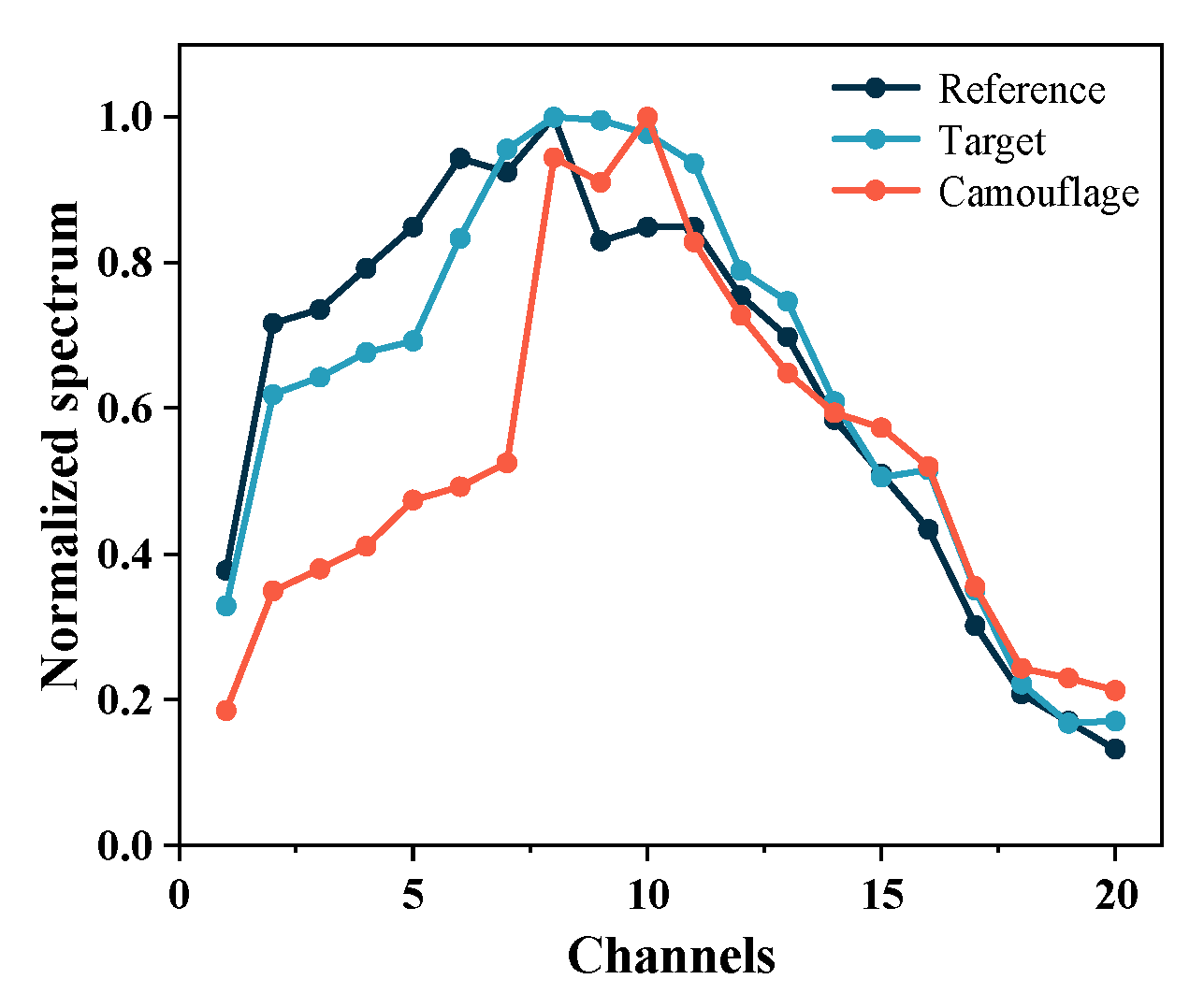
3.4. Characteristic Wavelength Selection and Spectral Restoration Result

Based on the decomposition result by the proposed method (including waveform accumulation), we used the intensity parameter in each channel to produce the target’s spectra. The target’s normalized spectra before and after being covered were composed of all 70 channels, as shown in Figure 10.

As Figure 10 shows, the normalized spectra of the same target differ greatly from the original spectra after being covered. However, the spectra should not change greatly if the target is only partly covered. Factors such as the “sub-footprint” effect [12] contribute to the occurrence of the phenomenon and make the subsequent target recognition and classification by the spectra difficult. Therefore, we utilized the improved waveform decomposition result and the proposed spectral extraction method to help distinguish the target, which can also be used in other applications such as point cloud identification.

According to the method described in Section 2.3.3, 11 indicators, including all waveform component parameters and all evaluation indicators for a single channel, were dimensioned using PCA.

Table 7. Eigenvalues and contributions of principal components of characteristic target spectra.

Component	Initial Eigenvalue			Dimensionality Reduction Process
	Eigenvalue	Contribution	Total Contribution	Eigenvalue	Contribution	Total Contribution
1	4.81	43.70%	43.70%	4.81	43.70%	43.70%
2	2.09	19.04%	62.74%	2.09	19.04%	62.74%
3	1.39	12.65%	75.38%	1.39	12.65%	75.38%
4	1.08	9.84%	85.22%	1.08	9.84%	85.22%
5	0.92	8.33%	93.55%	0.92	8.33%	93.55%
6	0.30	2.77%	96.32%
7	0.19	1.70%	98.01%
8	0.11	0.98%	99.00%
9	0.06	0.59%	99.58%
10	0.04	0.36%	99.94%
11	0.007	0.006%	100%

lists the results of PCA. The eigenvalues of the first five principal components were 4.81, 2.09, 1.39, 1.08, and 0.92, and the variance contributions were 43.70, 19.04, 12.65, 9.84, and 8.33%, for a cumulative contribution of 93.55%. Since the first five principal components covered 93.55% of the total raw data and were sufficient to represent that information, they were used to evaluate and cluster the wavelengths of each channel.

The pedigree diagram obtained by clustering is shown in Figure 11a. Since they were complex, we divided the pedigrees (70 channels) into categories in order, from three categories to seven categories, using the cluster function in MATLAB. Regardless of the categorical division, the intensity of the channel decomposition results in the first category were taken to compose the spectra of the two targets, as the first category contains the channels with the highest comprehensive evaluation. Figure 11b–g shows the feature spectra figures plotted by various divisions, where the abscissa represents the number of channels included in the first category among the total categories. It can be observed that when they were divided into three, five, and six categories, the spectra of the two targets could be distinguished intuitively. However, since the number of spectral channels was the largest when they were divided into three categories, we finally chose to divide all channels into three categories according to the comprehensive evaluation and restore the feature spectra by using the channels in the first of these categories.

When the channels were divided in three categories, there were 20 spectral channels in the first category: 600, 625, 630, 635, 650, 660, 665, 700, 735, 750, 770, 785, 795, 845, 865, 875, 900, 925, 935, 960, 935, and 960 nm. Before the 10th channel wavelength of 750 nm, the relative spectral intensity of the target plate was more than twice that of the camouflage net, showing an apparent difference (Figure 11c). After the 10th channel, the spectral intensity of both showed a decreasing trend with increasing wavelength, and their spectra were similar. Therefore, the characteristic spectra consisting of the 20 channels selected by comparison were sufficient to distinguish the target from the camouflage net. Moreover, these selected 20 channels comprised a wide range of spectra containing some of the wavelengths required to compose narrowband normalized difference vegetation indexes, such as NDLInr (670 nm, 784 nm) [38], NDLIne (719 nm, 784 nm) [39], and DLRner (686 nm, 703 nm, 751 nm) [36]. The selected channels and the selection method were proven to be valid by these two features.

The spectrum formed by the proposed spectral extraction method is shown in Figure 12. Intuitively, the selected wavelength avoids the influence of factors such as the “sub-footprint” effect, while different targets (camouflage net and target board) can be distinguished, and the characteristic spectral morphology of the same target is more similar, although there are specific differences in some wavelengths (735, 750, and 770 nm).

Table 8. The changes of correlation coefficient of targets’ spectrum before and after using the proposed method.

Spectrum	Target Uncovered vs. Target Covered	Target Uncovered vs. Camouflage Net	Target Covered vs. Camouflage Net
Before extraction	0.8945	0.7635	0.8766
After extraction	0.9526	0.6984	0.8530

shows the comparison of the correlation coefficient between spectra of the same target and two targets before and after the application of the proposed method, to illustrate its effectiveness.

It can be seen from Table 8 that the correlation coefficient of the same target significantly increased from 0.8945 to 0.9526, indicating that the proposed method can reduce the influence of interference factors and improve the spectral similarity of the target. Meanwhile, the correlation coefficient between the target and the camouflage net is reduced, indicating that the method can also reduce the spectral similarity of different targets. The proposed spectral extraction method is proven to be effective. The negative influence brought by being covered when distinguishing the different targets is reduced by the method.

4. Discussion

As described in this paper, we proposed a method for processing HSL 101-channel waveform data and prepared an experiment for detecting covered targets to verify the method. The purpose was to make up for the shortcomings of single and multi-wavelength channel waveform decomposition methods for hundred level spectral channel waveform decomposition, reduce the impact of adverse factors such as the “sub-footprint” effect on the retrieval of geometric and spectral information such as multi-target intensity and distance, and provide a new waveform data processing reference for future point cloud expansion, classification, and color identification applications. Most previous research on waveform data processing was conducted using a single wavelength, which seemed inadequate when dealing with HSL multi-channel data. Therefore, we attempted to process HSL waveform data by taking advantage of numerous channels. After eliminating a certain number of useless channels, we retrieved distance and intensity information through SCWD and MCMCD. Next, we selected the wavelength to retrieve the target spectral information by performing PCA on the waveform decomposition result and using its evaluation index and clustering.

First, it is innovative to eliminate useless channels by fitting the transmitter pulse. The HSL system used in the study included 101 channels from 550 to 1050 nm, with some channels containing a limited amount of useful information. Therefore, these channels must be removed before formally processing HSL data to prevent them from having a negative impact on the expected outcome. We set a threshold value to detect whether the maximum intensity value in all channels was greater than the threshold value, removed the channels with extremely low intensity, fitted them according to the transmitter pulse recorded by HSL, and removed poorly fitting channels. Since the data recorded by these channels cannot determine the center position of transmitter pulses, the actual distance of the target cannot ultimately be determined. After the above two steps, there were about 70 channels left from the 101 channels, which was still a high number and would not significantly impact the retrieval of target distance and spectral information. Next, according to the fitting results of transmitter pulses, we shifted the center positions of the transmitted pulses in all channels to the same starting point to ensure the consistency of waveform decomposition results and avoid misjudging the same target as two targets.

Second, from previous studies we learned about different waveform decomposition methods, and adopting the SND model, the layer-stripping strategy, and SOA for initiation and TR optimization for the SCWD step. The SND function model contains a Gaussian model, which is more suitable for asymmetric waveforms caused by unexpected factors in each detection step. The layer-stripping strategy and SOA are less affected by filtering and denoising and can obtain more accurate initial parameter sets. We adopted TR optimization rather than the commonly used LM because TR can constrain the optimization range of some parameters, which can be set according to the correct statistical result in SCWD and the practical conditions for the MCMCD step.

Next, we added the MCMCD step after the commonly used SCWD step. An index composed of the average distance difference between two adjacent targets, plus or minus its standard deviation, was used to judge whether the decomposition result of each channel was incorrect. Furthermore, the correct decomposition results, including FWHM and center position parameters, were counted as the initial supplementary parameters and the limitation range in TR optimization to help those wrong channels re-decompose, according to the core concept of the MCMCD step. After MCMCD, the decomposition results of most channels were within the threshold limit of the experimental scene settings, and the average value of the distance of each channel was taken as the measured target distance. Compared to the waveform accumulation method, although the WA method can improve the SNR and help reveal hidden and overlapping waveform components, the obtained results are not appropriate for some other channels in decomposition, and the accuracy can be improved by adding the MCMCD step. However, the WA method was integrated on FPGA hardware, while the FWHSL system in this paper can only obtain the original experimental data, which are processed uniformly after obtaining all experimental data. The calculation process of each part of the proposed method is separate, and the added steps for channel selection and spectral extraction are not integrated in the hardware. Moreover, the connection of many works is completed manual. Thus, the proposed method is bound to take a longer time than other methods. We calculated the time for data reading, transmitted pulse fitting, and the SCWD and MCMCD steps, which were 7.406773, 10.119411, 48.715824, and 48.404275 s, respectively.

Finally, we developed a new wavelength selection method and characteristic spectrum restoration method to retrieve the target’s spectral information. We performed PCA on 11 indicators, including two waveform component parameters, along with intensity, center position, pulse width, the skew coefficient of the SND model, and accuracy evaluation indexes of the decomposition results. We selected the top five principal components (whose total contribution was 93.55%) to evaluate and cluster all channels. These indicators took into consideration most of the information of all targets and other factors. At first, we did not know how many categories the clustering results should be divided into. By attempting to divide them into two to seven categories, we finally found that it was most appropriate to divide them into three categories, and we combined the intensity of all channels in the first category as the target characteristic spectrum. By comparison, we found that the spectra composed of these channels were very similar to those measured by the uncovered target. At the same time, there was a significant difference between the spectra of the target and the camouflage net. Furthermore, the selected wavelengths included some commonly used wavelengths that comprise vegetation indexes. We demonstrated the validity of our wavelength selection approach.

Currently, the 99% standard plate is commonly used in detecting target spectra with HSL to determine the spectral information of the target. However, the use of the standard plate may be limited in future applications based on practical scenarios. To achieve the purpose of distinguishing targets, a database can be collected by measuring various types of target spectra, then comparing them using our method to determine the targets. In the final results, the characteristic spectra of the targets are still very similar, whether covered or not, except for differences in some wavelengths. Still, more experiments should be performed to draw the appropriate conclusion.

5. Conclusions

In this paper, we propose a method to process 101-channel waveform data recorded by HSL to retrieve distance and spectral information of covered targets. This method takes advantage of HSL’s ability to record transmitter pulses and removes channels with little valid information in advance, utilizes the hidden information in all 101 channels, detects whether there are outliers in the waveform decomposition results based on the difference in distance between two adjacent targets, and provides erroneous channels with correct initial parameter sets for re-decomposition in the MCMCD step. Comparing the decomposition results with only SCWD and with SCWD and MCMCD, it was found that the distance retrieval results after MCMCD were closer to the actual distance designed in the experimental scenario, and the difference in distance between the two targets was improved from 39.36 to 44.83 cm, with a decrease in the REOA index from 0.1235 to 0.0037 and a reduction in distance deviation range (IOD) of 95.39%, which significantly reduced the number of outliers and the uncertainty of previous distance retrieval. Compared with the waveform accumulation method, the proposed method performed better for the remained 70 channels in terms of accuracy because the information hidden in the 101 channels was utilized. Finally, by applying PCA to score and cluster all channels, the characteristic wavelengths were selected, and the characteristic spectra of covered targets were plotted in order to avoid the negative influence of being covered. We successfully distinguished the targets from the camouflage network and found that the spectra of the targets, whether obscured or not, remained almost unchanged. This method was proven to be effective and applicable to waveform data processing of hundred level FWHSL.

In summary, this method effectively and successfully retrieves distance and spectral information of covered targets, effectively utilizes multiple HSL channels, and mines HSL waveform data to improve the accuracy of waveform decomposition and the detection of overlapping hidden components. Moreover, the method can be developed and used for HSL with more than 101 channels in the future, although it is not integrated with hardware and needs to be processed manually in successive steps, which takes more time than the integrated method. Next, we hope to integrate this method into the HSL system platform to achieve quicker processing time and produce a database of multiple target echo waveforms so that it can be widely applied to various scenes and targets. In addition, we will conduct a more in-depth study on the intensity of echoes and the variation in target spectra caused by the covering condition (e.g., the proportion of covered area).

References

1. Tan, K.; Cheng, X. Correction of Incidence Angle and Distance Effects on TLS Intensity Data Based on Reference Targets. Remote Sens. 2016, 8, 251. [Google Scholar] [CrossRef] [Green Version]
2. Mallet, C.; Bretar, F. Full-Waveform Topographic Lidar: State-of-the-Art. ISPRS J. Photogramm. Remote Sens. 2009, 64, 1–16. [Google Scholar] [CrossRef]
3. Wagner, W. Radiometric Calibration of Small-Footprint Full-Waveform Airborne Laser Scanner Measurements: Basic Physical Concepts. ISPRS J. Photogramm. Remote Sens. 2010, 65, 505–513. [Google Scholar] [CrossRef]
4. Wang, C.-K.; Tseng, Y.-H.; Wang, C.-K. A Wavelet-Based Echo Detector for Waveform LiDAR Data. IEEE Trans. Geosci. Remote Sens. 2016, 54, 757–769. [Google Scholar] [CrossRef]
5. Parrish, C.E.; Jeong, I.; Nowak, R.D.; Smith, R.B. Empirical Comparison of Full-Waveform Lidar Algorithms. Photogramm. Eng. Remote Sens. 2011, 77, 825–838. [Google Scholar] [CrossRef]
6. Chen, B.; Shi, S.; Gong, W.; Zhang, Q.; Yang, J.; Du, L.; Sun, J.; Zhang, Z.; Song, S. Multispectral LiDAR Point Cloud Classification: A Two-Step Approach. Remote Sens. 2017, 9, 373. [Google Scholar] [CrossRef] [Green Version]
7. Kukkonen, M.; Maltamo, M.; Korhonen, L.; Packalen, P. Comparison of Multispectral Airborne Laser Scanning and Stereo Matching of Aerial Images as a Single Sensor Solution to Forest Inventories by Tree Species. Remote Sens. Env. 2019, 231, 111208. [Google Scholar] [CrossRef]
8. Sumnall, M.J.; Hill, R.A.; Hinsley, S.A. Comparison of Small-Footprint Discrete Return and Full Waveform Airborne Lidar Data for Estimating Multiple Forest Variables. Remote Sens. Env. 2016, 173, 214–223. [Google Scholar] [CrossRef] [Green Version]
9. Lin, Y.; West, G. Retrieval of Effective Leaf Area Index (LAIe) and Leaf Area Density (LAD) Profile at Individual Tree Level Using High Density Multi-Return Airborne LiDAR. Int. J. Appl. Earth Obs. Geoinf. 2016, 50, 150–158. [Google Scholar] [CrossRef]
10. Bi, K.; Xiao, S.; Gao, S.; Zhang, C.; Huang, N.; Niu, Z. Estimating Vertical Chlorophyll Concentrations in Maize in Different Health States Using Hyperspectral LiDAR. IEEE Trans. Geosci. Remote Sens. 2020, 58, 8125–8133. [Google Scholar] [CrossRef]
11. Li, W.; Niu, Z.; Sun, G.; Gao, S.; Wu, M. Deriving Backscatter Reflective Factors from 32-Channel Full-Waveform LiDAR Data for the Estimation of Leaf Biochemical Contents. Opt. Express 2016, 24, 4771. [Google Scholar] [CrossRef] [PubMed]
12. Zhang, C.; Gao, S.; Li, W.; Bi, K.; Huang, N.; Niu, Z.; Sun, G. Radiometric Calibration for Incidence Angle, Range and Sub-Footprint Effects on Hyperspectral LiDAR Backscatter Intensity. Remote Sens. 2020, 12, 1–18. [Google Scholar] [CrossRef]
13. Chen, B.; Shi, S.; Sun, J.; Chen, B.; Guo, K.; Du, L.; Yang, J.; Xu, Q.; Song, S.; Gong, W. Using HSI Color Space to Improve the Multispectral Lidar Classification Error Caused by Measurement Geometry. IEEE Trans. Geosci. Remote Sens. 2021, 59, 3567–3579. [Google Scholar] [CrossRef]
14. Wang, B.; Song, S.; Shi, S.; Chen, Z.; Li, F.; Wu, D.; Liu, D.; Gong, W. Multichannel Interconnection Decomposition for Hyperspectral LiDAR Waveforms Detected From Over 500 m. IEEE Trans. Geosci. Remote Sens. 2022, 60, 1–14. [Google Scholar] [CrossRef]
15. Luo, B.; Yang, J.; Song, S.; Shi, S.; Gong, W.; Wang, A.; Du, L. Target Classification of Similar Spatial Characteristics in Complex Urban Areas by Using Multispectral LiDAR. Remote Sens. 2022, 14, 238. [Google Scholar] [CrossRef]
16. Hakala, T.; Suomalainen, J.; Kaasalainen, S. Full waveform active hyperspectral LiDAR. Int. Arch. Photogramm. Remote Sens. Spat. Inf. Sci. 2012, XXXIX-B7, 459–462. [Google Scholar] [CrossRef] [Green Version]
17. Suomalainen, J.; Hakala, T.; Kaartinen, H.; Räikkönen, E.; Kaasalainen, S. Demonstration of a Virtual Active Hyperspectral Lidar in Automated Point Cloud Classification. ISPRS J. Photogramm. Remote Sens. 2011, 66, 637–641. [Google Scholar] [CrossRef]
18. Chen, Y.; Li, W.; Hyyppä, J.; Wang, N.; Jiang, C.; Meng, F.; Tang, L.; Puttonen, E.; Li, C. A 10-Nm Spectral Resolution Hyperspectral LiDAR System Based on an Acousto-Optic Tunable Filter. Sensors 2019, 19, 1620. [Google Scholar] [CrossRef] [Green Version]
19. Hu, P.-L.; Chen, Y.-W.; Jiang, C.-H.; Lin, Q.-N.; Li, W.; Qi, J.-B.; Yu, L.-F.; Shao, H.; Huang, H.-G. Spectral Observation and Classification of Typical Tree Species Leaves Based on Indoor Hyperspectral Lidar. J. Infrared Millim. Waves 2020, 39, 372–380. [Google Scholar]
20. Song, S.; Wang, B.; Gong, W.; Chen, Z.; Lin, X.; Sun, J.; Shi, S. A New Waveform Decomposition Method for Multispectral LiDAR. ISPRS J. Photogramm. Remote Sens. 2019, 149, 40–49. [Google Scholar] [CrossRef]
21. Saini, T.S.; Baili, A.; Kumar, A.; Cherif, R.; Zghal, M.; Sinha, R.K. Design and Analysis of Equiangular Spiral Photonic Crystal Fiber for Mid-Infrared Supercontinuum Generation. J. Mod. Opt. 2015, 62, 1–7. [Google Scholar] [CrossRef]
22. Yang, H.; Han, F.; Hu, H.; Wang, W.; Zeng, Q. Spectral-Temporal Analysis of Dispersive Wave Generation in Photonic Crystal Fibers of Different Dispersion Slope. J. Mod. Opt. 2014, 61, 409–414. [Google Scholar] [CrossRef]
23. Eitel, J.U.H.; Magney, T.S.; Vierling, L.A.; Dittmar, G. Assessment of Crop Foliar Nitrogen Using a Novel Dual-Wavelength Laser System and Implications for Conducting Laser-Based Plant Physiology. ISPRS J. Photogramm. Remote Sens. 2014, 97, 229–240. [Google Scholar] [CrossRef]
24. Qin, Y.; Yao, W.; Vu, T.T.; Li, S.; Niu, Z.; Ban, Y. Characterizing Radiometric Attributes of Point Cloud Using a Normalized Reflective Factor Derived from Small Footprint LiDAR Waveform. IEEE J. Sel. Top. Appl. Earth Obs. Remote Sens. 2015, 8, 740–749. [Google Scholar] [CrossRef]
25. Zhang, C. Key Techniques of Data Processing of Hyperspectral LiDAR for Earth Detection. Ph.D. Thesis, University of Chinese Academy of Sciences, Beijing, China, 2021. [Google Scholar]
26. Yu, X.; Hyyppä, J.; Litkey, P.; Kaartinen, H.; Vastaranta, M.; Holopainen, M. Single-Sensor Solution to Tree Species Classification Using Multispectral Airborne Laser Scanning. Remote Sens. 2017, 9, 108. [Google Scholar] [CrossRef] [Green Version]
27. Carrea, D.; Abellan, A.; Humair, F.; Matasci, B.; Derron, M.H.; Jaboyedoff, M. Correction of Terrestrial LiDAR Intensity Channel Using Oren-Nayar Reflectance Model: An Application to Lithological Differentiation. ISPRS J. Photogramm. Remote Sens. 2016, 113, 17–29. [Google Scholar] [CrossRef]
28. Wagner, W.; Ullrich, A.; Ducic, V.; Melzer, T.; Studnicka, N. Gaussian Decomposition and Calibration of a Novel Small-Footprint Full-Waveform Digitising Airborne Laser Scanner. ISPRS J. Photogramm. Remote Sens. 2006, 60, 100–112. [Google Scholar] [CrossRef]
29. Neuenschwander, A.L. Evaluation of Waveform Deconvolution and Decomposition Retrieval Algorithms for ICESat/GLAS Data. Canadian J. Remote Sens. 2008, 34, S240–S246. [Google Scholar] [CrossRef]
30. Zhou, T.; Popescu, S.C.; Krause, K.; Sheridan, R.D.; Putman, E. Gold-A Novel Deconvolution Algorithm with Optimization for Waveform LiDAR Processing. ISPRS J. Photogramm. Remote Sens. 2017, 129, 131–150. [Google Scholar] [CrossRef]
31. Zhang, Z.; Xie, H.; Tong, X.; Zhang, H.; Tang, H.; Li, B.; Wu, D.; Hao, X.; Liu, S.; Xu, X.; et al. A Combined Deconvolution and Gaussian Decomposition Approach for Overlapped Peak Position Extraction from Large-Footprint Satellite Laser Altimeter Waveforms. IEEE J. Sel. Top. Appl. Earth Obs. Remote Sens. 2020, 13, 2286–2303. [Google Scholar] [CrossRef]
32. Bruggisser, M.; Roncat, A.; Schaepman, M.E.; Morsdorf, F. Retrieval of Higher Order Statistical Moments from Full-Waveform LiDAR Data for Tree Species Classification. Remote Sens. Environ. 2017, 196, 28–41. [Google Scholar] [CrossRef]
33. Shao, H.; Sa, B.; Li, W.; Chen, Y.; Liu, L.; Chen, J.; Sun, L.; Hu, Y. A Design and Implementation of Full-Waveform Hyperspectral LiDAR for Ancient Architecture Modelling. Infrared Laser Eng. 2022, 51, 20210786-1–20210786-10. [Google Scholar]
34. Soudarissanane, S.; Lindenbergh, R.; Menenti, M.; Teunissen, P. Scanning Geometry: Influencing Factor on the Quality of Terrestrial Laser Scanning Points. ISPRS J. Photogramm. Remote Sens. 2011, 66, 389–399. [Google Scholar] [CrossRef]
35. Hofton, M.A.; Minster, J.B.; Blair, J.B. Decomposition of Laser Altimeter Waveforms. IEEE Trans. Geosci. Remote Sens. 2000, 38, 1989–1996. [Google Scholar] [CrossRef]
36. Dash, J.; Curran, P.J. The MERIS Terrestrial Chlorophyll Index. Int. J. Remote Sens. 2004, 25, 5403–5413. [Google Scholar] [CrossRef]
37. Song, S.; Chen, Y.; Hu, H.; Hu, J.; Gong, Y.-M.; Shao, H. The Feasibility Study of Wavelength Selection of Multi-Spectral LIDAR for Autonomous Driving. J. Infrared Millim. Waves 2020, 39, 86–91. [Google Scholar] [CrossRef]
38. Gitelson, A.; Merzlyak, M.N. Spectral Reflectance Changes Associated with Autumn Senescence of Aesculus Hippocastanum L. and Acer Platanoides L. Leaves. Spectral Features and Relation to Chlorophyll Estimation. J. Plant Physiol. 1994, 143, 286–292. [Google Scholar] [CrossRef]
39. Barnes, E.M.; Clarke, T.R.; Richards, S.E.; Colaizzi, P.D.; Haberland, J.; Kostrzewski, M.; Waller, P.; Choi, C.R.E.; Thompson, T.; Lascano, R.J.; et al. Coincident Detection of Crop Water Stress, Nitrogen Status and Canopy Density Using Ground Based Multispectral Data. In Proceedings of the 5th International Conference Precis Agric, Bloomington, MN, USA, 16–19 July 2000. [Google Scholar]
Figure 1. (a) Architecture of HSL system. (b) Prototype of AOTF-HSL.
Remotesensing 14 05285 g001
Figure 2. Test results of transmitted pulse energy stability on white reflectance standard board with 99% reflectivity.
Remotesensing 14 05285 g002
Figure 3. (a) Ideal and (b,c) experimental scenarios. (d) Experimental equipment including camouflage web and target.
Remotesensing 14 05285 g003
Figure 4. Flowchart of 101-channel HSL data processing method for revealing components and extracting spectra.
Remotesensing 14 05285 g004aRemotesensing 14 05285 g004b
Figure 5. Process of selecting channels and fitting results of part of channel transmitter pulses of laser point, including qualified and unqualified channels. (a) Step 1: Select channels that exceed the pulse width threshold; (b) Step 2: Select channels that exceed the accuracy threshold. (c) Some bad fittings of transmitter pulse; (d) Some good fittings of transmitter pulse.
Remotesensing 14 05285 g005
Figure 6. Launching time calibration: (a) initial irregular transmitter pulse of each channel before calibration; (b) regular transmitter pulse of each channel after calibration.
Remotesensing 14 05285 g006
Figure 7. Comparison of SCWD and MCMCD. (a,f) Distance difference of all channels and outliers detected by thresholds. (be) Wrong waveform decomposition results by SCWD alone, and (gj) improved results by MCMCD corresponding to wrong channels.
Remotesensing 14 05285 g007aRemotesensing 14 05285 g007b
Figure 8. Results and comparison of two methods of distance retrieval. (ac) Box diagrams of distance of two targets and distance difference after SCWD and MCMCD. (d,e) Schematic diagram of each channel’s waveform data after SCWD and MCMCD. (f,g) Top view of decomposition results in channel–intensity–time after SCWD and MCMCD, respectively.
Remotesensing 14 05285 g008aRemotesensing 14 05285 g008b
Figure 9. Comparison of waveform accumulation method and proposed method: (a) accumulated waveform; (b) 930 nm waveform by SCWD; (c) 930 nm waveform by MCMCD.
Remotesensing 14 05285 g009
Figure 10. Comparison of target’s normalized spectra before and after being covered by two hyperspectral waveform decomposition methods: (a) proposed method; (b) waveform accumulation method.
Remotesensing 14 05285 g010
Figure 11. (a) Pedigree diagram obtained by clustering all channels and categories. (bg) Result of classifying channels into categories.
Remotesensing 14 05285 g011aRemotesensing 14 05285 g011b
Figure 12. Characteristic spectrogram of channel composition selected by clustering and classification after principal component analysis.
Remotesensing 14 05285 g012