Article

A Comparison of Random Forest Algorithm-Based Forest Extraction with GF-1 WFV, Landsat 8 and Sentinel-2 Images

1
Aerospace Information Research Institute, Chinese Academy of Sciences, Beijing 100094, China
2
University of Chinese Academy of Sciences, Beijing 100049, China
3
Key Laboratory of Earth Observation of Hainan Province, Hainan Research Institute, Aerospace Information Research Institute, Chinese Academy of Sciences, Sanya 572029, China
*
Author to whom correspondence should be addressed.
Remote Sens. 2022, 14(21), 5296; https://doi.org/10.3390/rs14215296
Submission received: 20 September 2022 / Revised: 9 October 2022 / Accepted: 13 October 2022 / Published: 22 October 2022

Abstract

:
Forests are an essential part of the ecosystem and play an irreplaceable role in maintaining the balance of the ecosystem and protecting biodiversity. The monitoring of forest distribution plays an important role in the conservation and management of forests. This paper analyzes and compares the performance of imagery from GF-1 WFV, Landsat 8, and Sentinel-2 satellites with respect to forest/non-forest classification tasks using the random forest algorithm (RF). The results show that in the classification task of this paper, although the differences in classification accuracy among the three satellite datasets are not remarkable, the Sentinel-2 data have the highest accuracy, GF-1 WFV the second highest, and Landsat 8 the lowest. In addition, it was found that remotely sensed data of different processing levels show little influence on the classification accuracy with respect to the forest/non-forest classification task. However, the classification accuracy of the top of the atmosphere reflectance product was the most stable, and the vegetation index has a marginal effect on the distinction between forest and non-forest areas.

1. Introduction

According to the Food and Agriculture Organization of the United Nations (FAO) [1], there is 4.06 × 10⁹ ha of forested area globally in 2020, accounting for about 31% of the total land area. As one of the most important components of terrestrial ecosystems, forests play an irreplaceable role in regulating climate change, concealing water, providing habitat for plants and animals, and maintaining ecological balance [2,3]. Forest monitoring is essential for cognizing the status and changes of forest resources and enhancing the management and utilization of forests [4,5,6].
The monitoring of forests is usually carried out by field surveys and remote-sensing monitoring. Field surveys, although more accurate, are time-consuming, labor-intensive, and expensive. It is not easy to repeat this method in a relatively short period of time. For places with poor reachability, field surveys are often hard to achieve. In contrast, remote-sensing monitoring provides a more practical, efficient, and effective method. Remote-sensing monitoring can obtain information on the spatial distribution of forests in a relatively short period of time through the analysis of satellite observation data. The development of earth observation technology has made the acquisition of satellite data faster and more convenient, thereby enabling the provision of important data support for the remote-sensing monitoring of forests.
Despite the fact that a large number of remote sensing satellites have been launched, Landsat series and Sentinel-2 data occupy a major position [7,8,9,10] with respect to forest monitoring in existing studies, thereby making an important contribution to medium-resolution forest research. On the one hand, these satellite data have high quality that can accurately reflect the spectral information of features and help to distinguish different features. On the other hand, thanks to free and open-access policies [11,12,13,14], especially the openness of the Google Earth Engine (GEE) platform [15,16], it has become faster and easier for users to obtain remote-sensing images of the area of interest.
In the existing forest extraction work, particularly for large-scale (e.g., global-scale) forest information extraction, Landsat 8 (L8) and Sentinel-2 (S2) have achieved high forest classification accuracy as common data sources. Zhang et al. [17] released the 2018 global forest cover product GFC30 with an overall accuracy of 90.94%. The University of Maryland’s Global Analysis and Discovery (GLAD) lab released a series of 30 m global forest thematic products [2,18,19,20,21], including TreeCover2000, TreeCover2010, Global Forest change, etc.
Similar to Landsat and sentinel satellites, the Gaofen-1 (GF-1) wide field view (WFV) satellite provides data with high spatial and temporal resolutions, which can provide vital data support for forestry monitoring. By combining GF-1 WFV multispectral features, fused NDVI time series features, and phenological parameters, Xu et al. [22] used a random forest (RF) classification algorithm to classify forests in the eastern part of Hubei Province and achieved high classification accuracy (98.68%). Yin et al. [23] used the kernel principal component analysis (KPCA) method to detect forest changes in Yajiang County in Sichuan Province and achieved an overall accuracy of 89.27%. Integrating the land surface phenological metrics and text features of forest canopies on tree species identification based on GF-1 WFV data, Xu et al. [24] extracted categories of forest tree species in northeast China with an accuracy of 85.13%. Wu et al. [25] extracted the forest fires that occurred in 2018 in the Daxing’anling Khanma Nature Reserve with an extraction accuracy better than 94%.
Remote-sensing images are easily accessible. However, different satellites provide data at different processing levels, such as digital number (DN), top of atmosphere reflectance (TOA), and surface reflectance (SR). Furthermore, there are subtle differences between different satellites at the same data-processing level. For example, the Level 1 products of S2 and GF-1 WFV provide TOA and DN data, respectively, while the Level 1 image of L8 is radiometrically calibrated and presented in DN units [26]. Therefore, pre-processing of the downloaded data is usually required before information extraction [27,28,29], such as radiometric correction and atmospheric correction, to correct the effects on the spectra due to sensor errors, atmospheric conditions, and other factors. Pre-processing accounts for a large amount of the workload in the forest extraction task, yet few studies have examined the effect of the processing level of remote-sensing images on forest extraction accuracy.
This paper is designed to analyze and compare the performance of forest classification applied to GF-1 WFV, L8, and S2 images. In addition, the effects of different data-processing levels, spectral bands, and vegetation indices on the accuracy of the extracted forests from the remote-sensing images are explored. In this study, the RF algorithm was used to classify forests from images of different optical data sources in 23 different study areas. This study includes the following three aspects. First, the effects of different processing levels on the accuracy of extracting forests were estimated with GF-1 WFV and Landsat 8 images. Then, different bands and vegetation indices (VI) of Sentinel-2 and Landsat 8 data were used to assess the potential advantages of vegetation indices and different bands in forest classification. Finally, the performance of the three satellite datasets—GF-1 WFV, Landsat 8, and Sentinel-2—in forest/non-forest (FNF) classification tasks was analyzed and compared based on the classification results.

2. Materials and Methods
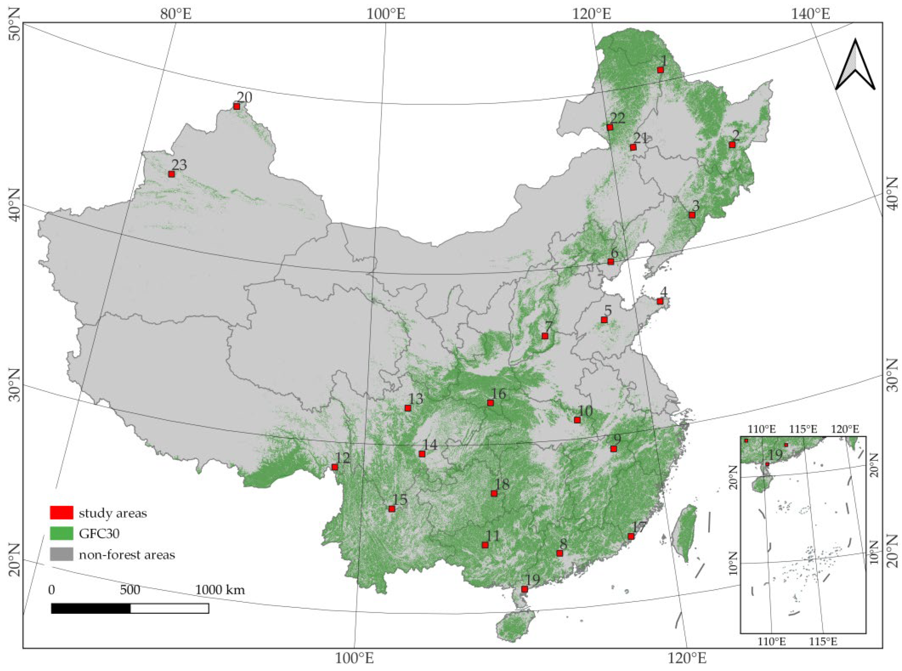
2.1. Study Area

In this paper, 23 typical locations in distinct regions were selected as study areas, each of which has a size of 38.4 km × 38.4 km. As shown in Figure 1, all 23 study areas are in China. These study areas with different topographic features and climatic characteristics are distributed in various regions.
To ensure the uniqueness of the vegetation characteristics in the study area, first, 23 GF-1 WFV images located in different vegetation zones were downloaded by referring to the Chinese vegetation zones [30]. Then, several existing medium-resolution forest products [31,32,33,34,35,36,37] were referred to, and the positions with the greatest inconsistency with respect to the forest products in the 23 images were selected separately.
The L8 and S2 images were acquired according to the determined study area locations. For the same study area, cloud-free remote-sensing images of the green season with similar acquisition dates were selected as far as possible to reduce the influence on the classification results in terms of atmospheric conditions, plant phenology, soil moisture, and environmental changes. Both training and testing samples were generated using a stratified random sampling method and interpreted by professionals. The number of sample points in each study area is shown in Figure 2.
However, it is hard to collect cloud-free data with similar acquisition dates, especially in regions with lower latitudes strongly influenced by the monsoon climate. Therefore, although we have relaxed the data collection time to the whole growing season in some areas, it is still impossible to collect data from all three satellites. Most of the images used in this study were acquired in the 2020 green season. Due to the narrower swath width (185 km) and longer revisit time (16 days) of Landsat 8 compared to S2 and GF-1 WFV, cloud-free images in the 2020 growing season were not available for some areas. Therefore, L8 images in these study areas are replaced with images form the 2019 growing season with similar phenology. Table 1 shows the data collected for the 23 study areas.

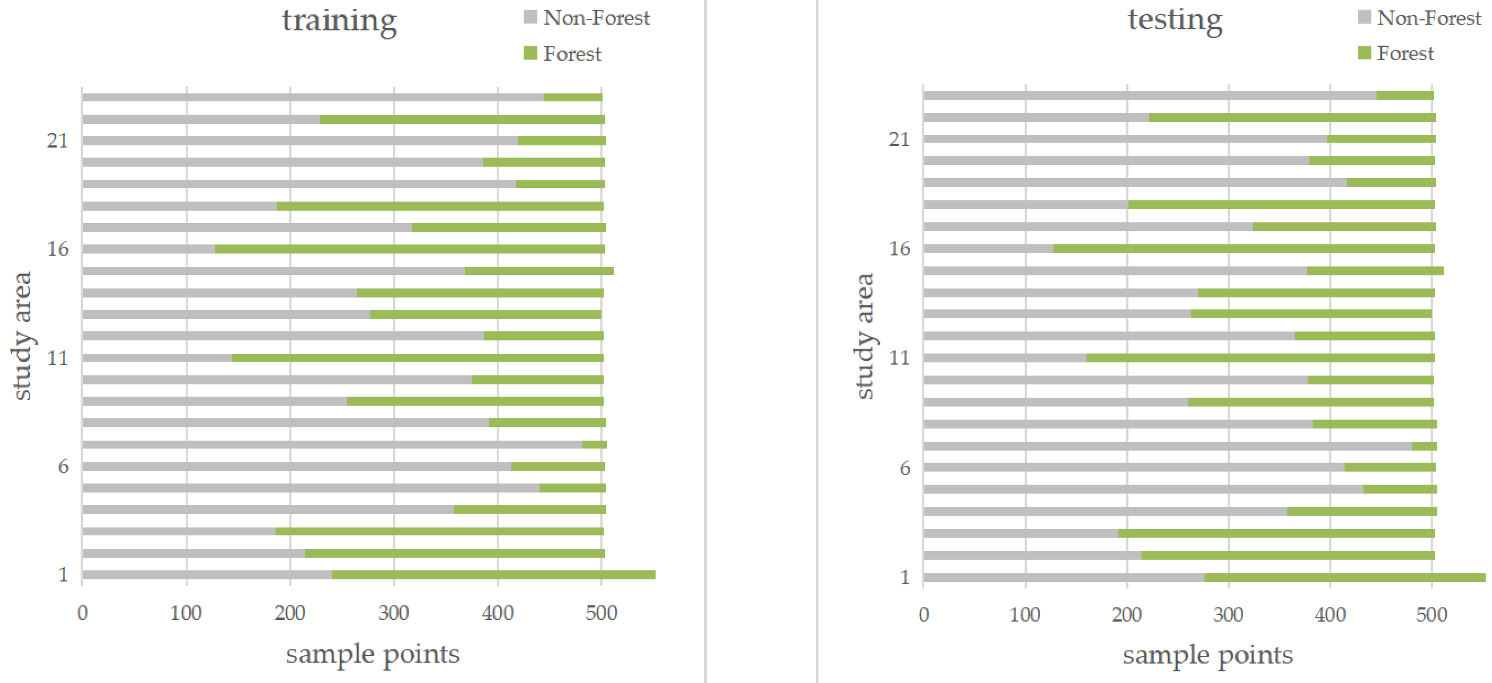
2.2. Remote-Sensing Data

2.2.1. GF-1 WFV Imagery

The GF-1 satellite was launched in April 2013 and it carries 2 high-resolution cameras and 4 wide-field view cameras. The WFV cameras with a swath width of 800 km have a temporal resolution of 4 days. The WFV data have 4 bands with a spatial resolution of 16 m, including red (R), green (G), blue (B), and near-infrared (NIR) bands. The GF-1 WFV data used in this paper are all L1-level products downloaded from China Center for Resources Satellite Data and Application (http://www.cresda.com/CN/, (accessed on 20 September 2022)) with system-level geometric corrections. The processing of the GF-1 WFV data mainly involves radiometric calibration, atmospheric correction, orthorectification correction, and spatial alignment. Four processing levels of DN, Radiance (Rad), TOA, and surface reflectance (SR) data were finally obtained.

2.2.2. Landsat 8 Imagery

Landsat series satellite data are widely used for forest cover mapping. In this paper, Landsat 8 Collection2 Level 1 and Level 2 data were downloaded from the United States Geological Survey (USGS) website (https://earthexplorer.usgs.gov/, (accessed on 20 September 2022)). The Level 1 data are radiometrically corrected and orthorectified products. Rad and TOA reflectance can be obtained very easily from Level 1 data based on metadata information. Level 2 consists of the surface reflectance product with atmospheric correction based on Level 1 product to eliminate atmospheric influence. L8 data have 11 bands, of which only 6 bands with 30 m resolution are used in this paper, including B, G, R, NIR, and 2 short-wave infrared (SWIR) bands. Then, the downloaded L1C data were atmospherically corrected and topographically corrected using the Snap plug-in Sen2Cor released by ESA to finally obtain the SR data.

2.2.3. Sentinel-2 Imagery

The S2 constellation consists of two satellites with a wide swath width (290 km) and high revisit times (10 days at the equator with one satellite, and 5 days with 2 satellites). The USGS website provides the L1C level product data with radiometric calibration, geometric refinement correction, and spatial alignment. The downloaded L1C data were then atmospherically corrected and topographically corrected using the Snap plug-in Sen2Cor released by ESA to finally obtain the Level 2A SR data. S2 data are available in 13 higher spatial resolution (10 m, 20 m, and 60 m) bands. In this work, 10 bands of S2 were utilized, including 4 bands with 10 m resolution (B, G, R, and NIR bands) and 6 bands with 20 m resolution (2 SWIR and four red edge (RE) bands).

2.3. Vegetation Indices

VIs are commonly used features in forest extraction tasks [38,39]. In this paper, six popular vegetation indices were selected (as shown in Table 2).

2.4. Methods

  • Classification methods
With advantages in handling multidimensional data, multicollinearity, and insensitivity to overfitting [47], RF algorithms prevail in medium-resolution image classification [18,34,48]. Moreover, RF algorithm is insensitive to noise and strongly robust, showing superior performance over other methods [49], especially in large-scale land use/land cover classification. In this paper, a pixel-based RF classification algorithm is used to distinguish FNF regions. All the experiments were implemented using libraries such as Scikit-learn, Rasterio, and Geopandas based on Python.
  • Accuracy assessment
Overall accuracy (OA), F1 score (F1), coefficient of variation (V), mean OA (mOA), and mean F1 (mF1) are used to assess the classification results. These metrics are calculated as follows:
OA = T N + T P T N + T P + F N + F P
F 1 = 2 × T P 2 × T P + F N + F P
V X = σ X ¯
mOA = i = 1 n O A i n
mF 1 = i = 1 n F 1 i n
where true positive (TP) and true negative (TN) indicate the number of true forest and true non-forest data being predicted correctly, respectively; false negative (FN) and false positive (FP) denotes the number of true forest and true non-forest data being predicted incorrectly, respectively. σ and X ¯ denote the standard deviation and mean value of X , respectively. Here, X indicates OA or F1 score for different study areas. i is the i-th study area and n is the number of study areas.
  • Setting of the classifier
Compared with the S2, L8 lacks the RE bands, while GF-1 WFV lacks both the RE and the SWIR bands. To verify the influence of the RE and SWIR bands on FNF classification, different band sets are designed in this work, as shown in Table 3.
Due to the different resolutions of satellite data from different data sources, the S2 and GF-1 WFV images are resampled to 30 m resolution and then classified to facilitate the comparison of the three data sources in forest extraction (i.e., the results in Section 3.3). Other than that, both Section 3.1 and Section 3.2 use the original resolutions of the image data.

3. Results and Discussions

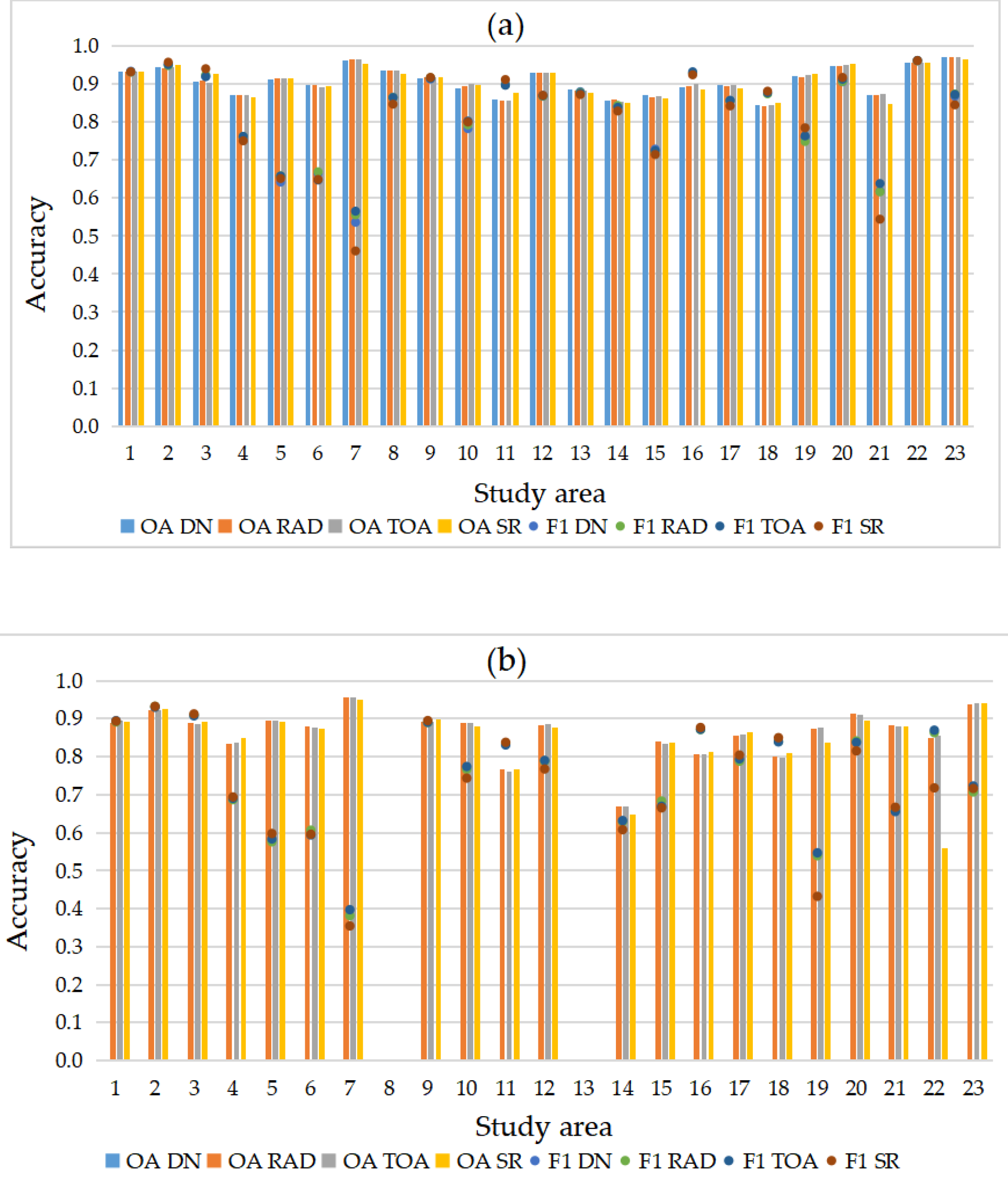
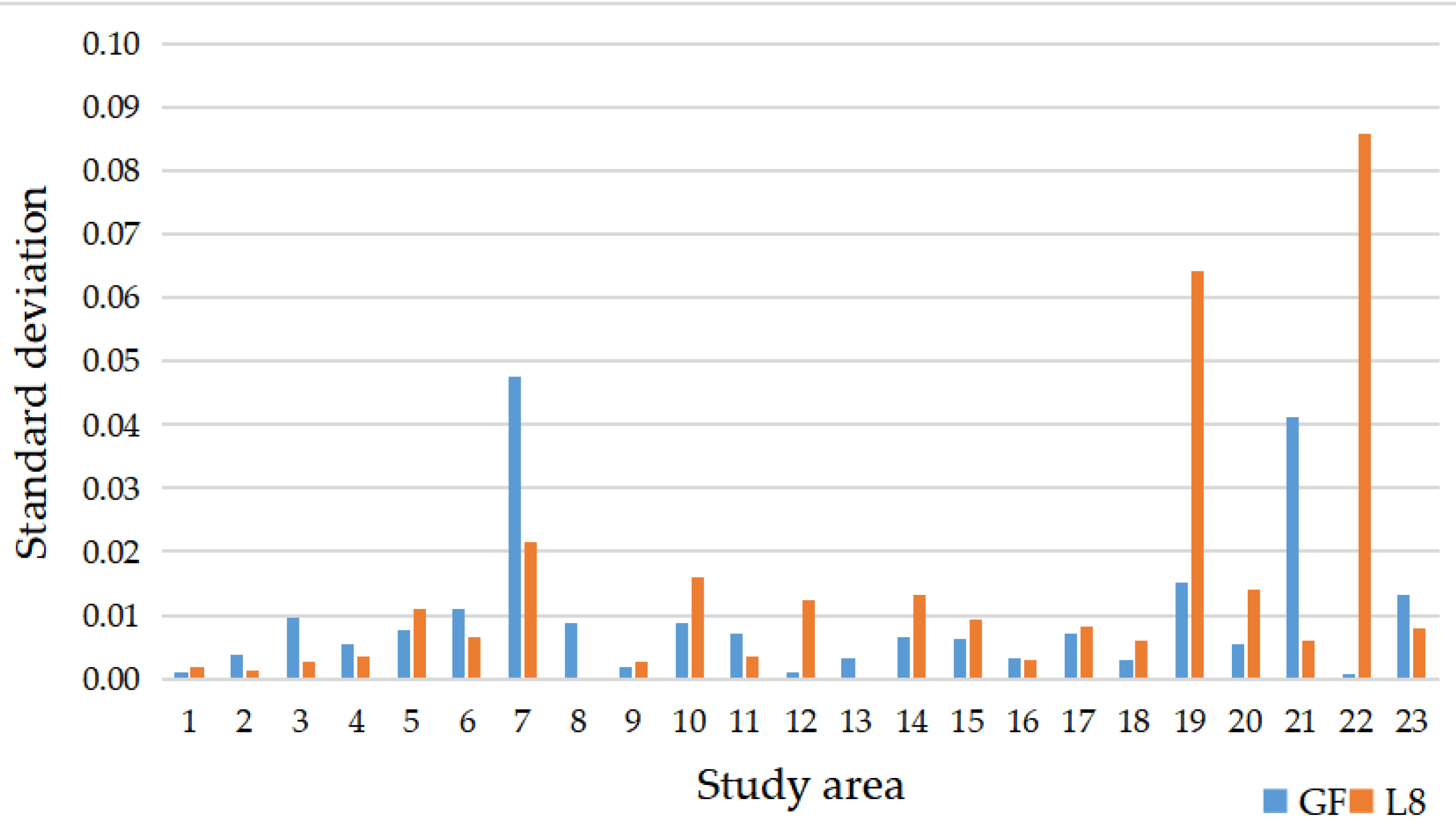
3.1. Forest Classification with Remotely Sensed Images at Different Processing Levels

This section compares the effects of four processing levels on the FNF classification results. These four levels include DN, RAD, TOA, and SR, which are typically the intermediate results of the pre-processing process.
The experimental results from the GF-1 WFV and L8 data show that different processing levels can achieve high classification accuracies in the FNF classification tasks. As shown in Figure 3, the classification results of different processing levels of the data from different areas have a consistent trend of variation. For example, the classification accuracy at all levels in area 10 is high simultaneously, while that in area 11 is low. For the same study area, the results extracted from the data at different processing levels do not differ significantly in terms of metric OA, but the difference is more obvious in some study areas regarding the F1 score. As illustrated in Figure 4, the standard deviation of the data results at different levels in four areas—7, 19, 21, and 22—was significantly larger than that in other study areas.
The difference in the F1 scores between the GF-1 WFV data in areas 7 and 21 was highly significant. The accuracy of the results extracted from the TOA reflectance in area 7 was the highest and the classification accuracy of the SR was the lowest, with a difference of 10.45% in the F1 score and 2.82% in the OA. Similar to the metric of area 7, the classification accuracy of the OA and the F1 score of the TOA data in area 21 were higher than those of SR by 1.11% and 9.38%, respectively.
Similar to the characteristics of GF-1 WFV, L8 shows the highest classification accuracy regarding TOA reflectance in area 19 and area 22. The classification accuracy of the TOA reflectance in area 19 was 3.77% and 11.45% higher than the minimum classification accuracy of the OA and F1, respectively. The accuracies of area 22’s TOA reflectance were 29.56% and 15.19% higher than the minimum metrics in terms of the OA and F1, respectively.
Although there are considerable differences in the classification results between processing levels in some areas, the effects of different processing levels on the FNF classification results do not show a great difference, as indicated in Table 4. The classification of the TOA reflectance shows the highest classification accuracy (i.e., the higher OA and F1 scores) compared to the data of other processing levels. The mOA and mF1 of GF-1 WFV are 90.81% and 82.78%, respectively, and those of L8 are 86.27% and 74.84%, respectively. Furthermore, the F1 scores of the TOA classification results with smaller VOA and VF1 indicate that the TOA is more stable in the FNF classification and slightly outperforms the results of other pre-processing levels. Although the difference in classification accuracy was slightly higher for L8 compared to the GF-1 WFV data at different processing levels, this difference was less than 2% for both mOA and mF1 score.

3.2. Forest/Non-Forest Classification with Multispectral Data

As shown in Table 5, the classification results for L8 and S2 demonstrate that the effects of SWIR and RE bands on FNF classification are positive, and the influence of the vegetation index on the classification results is marginal. Taking the S2 image as an example, exp1 with only B, G, R, and NIR bands achieves the lowest classification accuracy, with OA and F1 scores of 87.42% and 77.13%, correspondingly. The use of the RE band and SWIR band led to some improvement in classification accuracy. In particular, the classification accuracy of the simultaneous use of both bands is the largest, with OA and F1 scores reaching 88.62% and 79.53%, respectively, an improvement of 1.20% and 2.40%. However, the classification results indicate that the effect of the vegetation index on the FNF classification is remarkably slight, with the maximum effects on the OA and F1 at 0.28% and 0.42%, respectively.
The feature importance of each experiment was highly consistent (as shown in Figure 5 and Figure 6). Among the predictors of each satellite dataset, the R band ranks the highest in importance, followed by the B and G bands. The importance of the characteristics of B, G, and R decreases dramatically with the joining of other bands and vegetation indices but remains above 10% overall and is significantly higher than other bands and vegetation indices. The importance of the vegetation indices did not exceed 10%. The feature importance of the NDVI, sr, and ARVI was comparable in the same group of experiments and higher than that of SIPI, GNDVI, and EVI.

3.3. Assessment of Forest Classification Results with Different Sensors

Some study areas were removed to avoid inconsistent classification results due to data quality, location errors, and temporal phase differences. The classification results of nine study areas were finally retained to compare the classification results of the different sensor images. We compare the classification results from two perspectives: the original spatial resolution (OSR) and 30 m spatial resolution (30 m). The OSR means that each dataset keeps its original resolution unchanged, and 30 m resolution means that the data from different sources are resampled to 30 m spatial resolution by bilinear interpolation, the same as the L8 spatial resolution.
The experimental results show that the classification accuracies of the FNF for each sensor dataset are fairly comparable, as shown in Table 6. The differences in OA and F1 scores for the OSR and 30 m resolution (30 m) were about 1% and 3%, respectively. However, the S2 images slightly outperform the other images from GF-1 WFV and L8. The F1 scores of the S2 classification results were 81.12% and 81.44% for the OSR and 30 m resolution, which were 0.99% and 2.40% higher than GF-1 WFV, while being 2.81% and 3.13% higher than L8.
Moreover, the performance of each sensor dataset varies markedly in different study areas, as shown in Figure 7. In most of the study areas (e.g., study area 9 and study area 18), the classification results of each sensor dataset show high accuracy, and the accuracy differences were minimal. Nevertheless, part of the study areas displayed greater differences in the classification results of different satellite data, such as the maximum differences of up to 20% and 14% in the F1 score in study areas 21 and 23, respectively.
Figure 8, Figure 9, Figure 10 and Figure 11 display the overlay of the different sensor classification results for study areas 21, 9, 23, and 22, respectively. F and NF signify forest and non-forest regions in all the three satellite data classification results, respectively. OS/OL/OG represents only the classification results of S2/L8/GF considered as forest areas. OSN/OLN/OGN indicates that only the classification results of S2/L8/GF are considered non-forest. Columns A–B are the true images of the subregions. In each column, i represents the true images (the true images are from the ESRI satellite map built using the QGIS software, except for Figure 8 (study area 21, where the ESRI satellite map is not an image of the growing season) from Sentinel-2) and ii–iv represent the effect of the superimposition of the true images with the GF, L8, and S2 detection results, respectively.
Figure 8 shows the classification results for area 21 (121.64–122.17°E, 46.29–46.66°N), where the data acquisition time for all three satellites is July 2020, with a maximum time gap of 15 days. It is evident that there is a greater inconsistency in the classification results, while it is also clear that this is the study area with the greatest inconsistency among all the study areas. The classification results of each satellite image exhibit serious commissions and omissions, as shown by the pink and orange markers. In sub-area A, GF-1 WFV and L8 data misclassified agricultural land as forest and S2 misclassified grassland as forest. In sub-region B, GF-1 WFV has more omissions than L8, and S2 has more obvious commissions.
The main reasons for the variations in the classification results may be twofold. On the one hand, this study selects the study areas with strong inconsistency in classification among publicly available forest products, indicating that it is more problematic to distinguish the FNF in these areas. On the other hand, the bands of each satellite dataset are distinct. Section 3.2 suggests that the improvement of the bands is dramatic. Whereas the GF-1 WFV dataset has the fewest band compared to S2 and L8. Therefore, there may be some potential weaknesses in the areas where the classification is more difficult.
Although there is a large variation in the performance of the sensors in some study areas, in general, the overall distribution of the detections of the data from the satellites is in good agreement. Area 9′s (116.87–117.31°E, 29.00–29.38°N; shown in Figure 9) images were acquired in September 2020 with a maximum time difference of 3 days. However, the sensor data exhibit some pixel-level variability at the forest edges (as indicated by the yellow markers in subregions A and B of Figure 9). Among them, the edge discrepancy in subregion A is linear and mainly originates from the inconsistency between GF-1 WFV and other data results, which most likely originates from the location discrepancy between the remote-sensing data, and despite geometric correction and spatial alignment, it is still difficult to eliminate the location error. Despite the large differences in the performance of the sensors in some of the study areas, the overall distribution of the classification results of the data from the satellites is reasonably consistent.
Similar to area 9, area 23 (82.49–83.07°E, 43.91–44.32°N; Figure 10) showed similar edge effects. The forest locations derived from the three sensors’ data show some positional offsets (as shown in subarea A of Figure 10). Further, the forest extracted from the GF-1 WFV data is wider than the forest width extracted from the S2 and L8 images. The comparative analysis with the original images revealed that this is mainly due to image distortion and positional differences. The positional error between images leads to inconsistent classification results between the data of different sensors, but this difference is visually acceptable.
Except for image distortion and positional differences, the classification results for study area 23 also suffer from mountain shadows. As displayed in subarea B of Figure 10, the pink part indicates that non-forest areas are confused as forest areas. This region is located on the shaded slope of the mountain. As influenced by the shading of the mountain, this area shows spectral characteristics similar to the forest. However, it is clear that the images from different sensors are variously affected by the mountain shadow. The shadow shows the least impact on S2 and the greatest impact on L8. The L8 dataset was acquired on 21 September 2020, later than the other two satellite data, so we speculate that this difference is not only influenced by observation angle but also by the solar altitude angle.
The position error between images leads to inconsistent classification results between the sensor data, but this difference is visually acceptable. The impact on the classification results is worse due to spectral features, acquisition timing, etc. As shown in Figure 11 (study area 22; 119.92–120.45°E, 47.68–48.04°N), the L8 and S2 data suffer from significantly higher errors over this study area. The GF-1 WFV, L8, and S2 images for study area 22 were acquired on 21 August 2020, 13 September 2020, and 11 September 2020, respectively. The L8 and S2 images have severe classification errors, while the GF-1 WFV image behaves optimally. This result was probably influenced by the temporal phase difference. The data acquisition time of L8 is close to that of S2, but the classification result of S2 is better. The biggest difference between the two is the spectrum including the spectral features and the number of bands. Therefore, we speculate that the differences in the classification results between S2 and L8 are probably influenced by spectral differences.

4. Conclusions

The experiments in this study were set up to compare and analyze the ability of GF-1 WFV, L8, and S2 multispectral sensors with respect to FNF differentiation under different geographical environments. This study carefully analyzed the effects of different processing levels, band settings, and VIs on FNF classification accuracy.
There is a certain degree of inconsistency in the classification results of each sensor dataset in different study areas, and this inconsistency is usually caused by spatial positioning errors (including geometric correction/image alignment errors, image distortion, etc.) and physical differences between different datasets. However, the classification results of each sensor in the same study area had high spatial consistency. The conclusions drawn from this study are as follows.
(1)
The performance of the remote-sensing data of different processing levels in the FNF classification tasks did not differ significantly. However, concerning the stability of the classification accuracy at different processing levels, the classification accuracy of the TOA data is more stable and slightly better than that of the data at other processing levels.
(2)
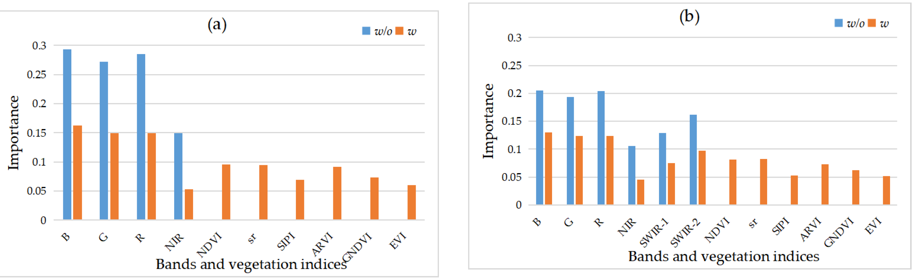
The SWIR and the RE bands are positive for the improvement of forest classification accuracy. The lack of these bands may cause some negative results in classifications. Although VIs can indicate vegetation, they do not contribute significantly in the FNF classification task in this paper.
(3)
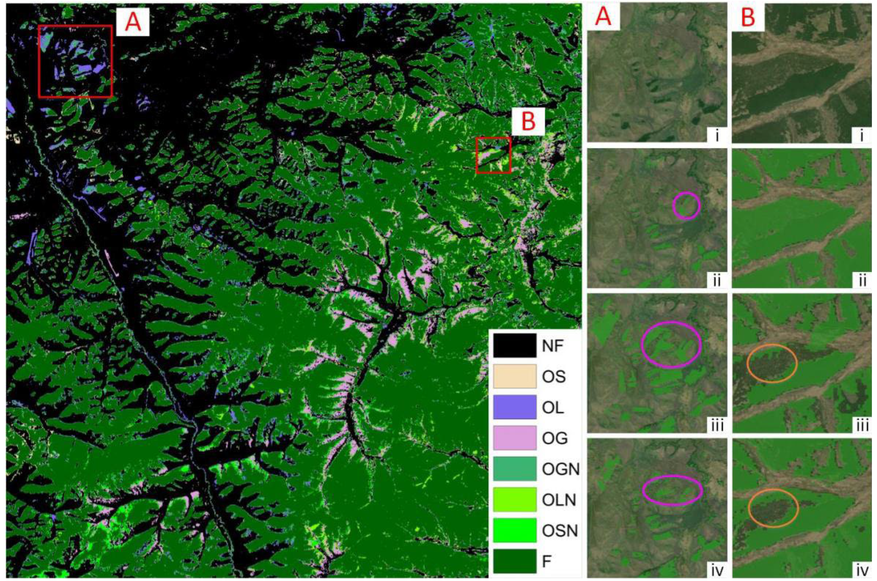
Of the three data sources compared, S2 yields the highest FNF differentiation ability at both the OSR and 30 m resolution, followed by GF-1 WFV and L8. Nevertheless, the three satellite images of GF-1 WFV, L8, and S2 show comparable abilities in distinguishing forest and non-forest areas. For example, the FNF OA of the GF-1 WFV, L8, and S2 data at the OSR did not differ significantly, yielding values of 89.72%, 88.61%, and 89.53%, respectively. Additionally, there is little difference with respect to the F1 scores, yielding values of 80.13%, 78.31%, and 81.12%.

Author Contributions

Conceptualization, X.P., G.H., G.W. and R.Y.; methodology, X.P.; experiments, X.P., W.S., R.Y. and T.L.; data curation, X.Z., G.W.; writing—original draft preparation, X.P.; writing—review and editing, G.H.; project administration, G.H. All authors have read and agreed to the published version of the manuscript.

Funding

This research was funded by the Strategic Priority Research Program of the Chinese Academy of Sciences, grant number XDA19090300; the program of the National Natural Science Foundation of China, grant number 61731022; the Second Tibetan Plateau Scientific Expedition and Research Program (STEP), grant number 2019QZKK030701; and Chinese Academy of Sciences Network Security and Informatization Special Project, grant number CAS-WX2021PY-0107-01.

Data Availability Statement

Not applicable.

Acknowledgments

The authors thank the anonymous reviewers and the editors for their valuable comments to improve our manuscript.

Conflicts of Interest

The authors declare no conflict of interest.

References

  1. Global Forest Resources Assessment 2020. Available online: https://www.fao.org/forest-resources-assessment/2020/en/ (accessed on 9 October 2022).
  2. Hansen, M.C.; Potapov, P.V.; Moore, R.; Hancher, M.; Turubanova, S.A.; Tyukavina, A.; Thau, D.; Stehman, S.V.; Goetz, S.J.; Loveland, T.R.; et al. High-resolution global maps of 21st-century forest cover change. Science 2013, 342, 850–853. [Google Scholar] [CrossRef] [PubMed] [Green Version]
  3. White, J.C.; Wulder, M.A.; Hermosilla, T.; Coops, N.C. Satellite time series can guide forest restoration. Nature 2019, 569, 630. [Google Scholar] [CrossRef] [PubMed] [Green Version]
  4. De Keersmaecker, W.; Rodríguez-Sánchez, P.; Milencović, M.; Herold, M.; Reiche, J.; Verbesselt, J. Evaluating recovery metrics derived from optical time series over tropical forest ecosystems. Remote Sens. Environ. 2022, 274, 112991. [Google Scholar] [CrossRef]
  5. Cardille, J.A.; Perez, E.; Crowley, M.A.; Wulder, M.A.; White, J.C.; Hermosilla, T. Multi-sensor change detection for within-year capture and labelling of forest disturbance. Remote Sens. Environ. 2022, 268, 112741. [Google Scholar] [CrossRef]
  6. Bullock, E.L.; Healey, S.P.; Yang, Z.; Houborg, R.; Gorelick, N.; Tang, X.; Andrianirina, C. Timeliness in forest change monitoring: A new assessment framework demonstrated using Sentinel-1 and a continuous change detection algorithm. Remote Sens. Environ. 2022, 276, 113043. [Google Scholar] [CrossRef]
  7. Grabska, E.; Hostert, P.; Pflugmacher, D.; Ostapowicz, K. Forest Stand Species Mapping Using the Sentinel-2 Time Series. Remote Sens. 2019, 11, 1197. [Google Scholar] [CrossRef] [Green Version]
  8. Hościło, A.; Lewandowska, A. Mapping Forest Type and Tree Species on a Regional Scale Using Multi-Temporal Sentinel-2 Data. Remote Sens. 2019, 11, 929. [Google Scholar] [CrossRef] [Green Version]
  9. Uday, P.; Asamaporn, S.; Dario, S.; Sukan, P.; Kumron, L.; Amnat, C. Topographic Correction of Landsat TM-5 and Landsat OLI-8 Imagery to Improve the Performance of Forest Classification in the Mountainous Terrain of Northeast Thailand. Sustainability 2017, 9, 258. [Google Scholar] [CrossRef] [Green Version]
  10. Chen, S.; Woodcock, C.E.; Bullock, E.L.; Arévalo, P.; Torchinava, P.; Peng, S.; Olofsson, P. Monitoring temperate forest degradation on Google Earth Engine using Landsat time series analysis. Remote Sens. Environ. 2021, 265, 112648. [Google Scholar] [CrossRef]
  11. Turner, W.; Rondinini, C.; Pettorelli, N.; Mora, B.; Leidner, A.K.; Szantoi, Z.; Buchanan, G.; Dech, S.; Dwyer, J.; Herold, M.; et al. Free and open-access satellite data are key to biodiversity conservation. Biol. Conserv. 2015, 182, 173–176. [Google Scholar] [CrossRef]
  12. Woodcock, C.E.; Allen, R.; Anderson, M.; Belward, A.; Bindschadler, R.; Cohen, W.; Gao, F.; Goward, S.N.; Helder, D.; Helmer, E. Free Access to Landsat Imagery. Science 2008, 320, 1011. [Google Scholar] [CrossRef]
  13. Phiri, D.; Morgenroth, J. Developments in Landsat Land Cover Classification Methods: A Review. Remote Sens. 2017, 9, 967. [Google Scholar] [CrossRef] [Green Version]
  14. Dwyer, J.L.; Roy, D.P.; Sauer, B.; Jenkerson, C.B.; Zhang, H.K.; Lymburner, L. Analysis Ready Data: Enabling Analysis of the Landsat Archive. Remote Sens. 2018, 10, 1363. [Google Scholar] [CrossRef]
  15. Tamiminia, H.; Salehi, B.; Mahdianpari, M.; Quackenbush, L.; Adeli, S.; Brisco, B. Google Earth Engine for geo-big data applications: A meta-analysis and systematic review. ISPRS J. Photogramm. Remote Sens. 2020, 164, 152–170. [Google Scholar] [CrossRef]
  16. Gorelick, N.; Hancher, M.; Dixon, M.; Ilyushchenko, S.; Thau, D.; Moore, R. Google Earth Engine: Planetary-scale geospatial analysis for everyone. Remote Sens. Environ. 2017, 202, 18–27. [Google Scholar] [CrossRef]
  17. Zhang, X.; Long, T.; He, G.; Guo, Y.; Yin, R.; Zhang, Z.; Xiao, H.; Li, M.; Cheng, B. Rapid generation of global forest cover map using Landsat based on the forest ecological zones. J. Appl. Remote Sens. 2020, 14, 022211. [Google Scholar] [CrossRef]
  18. Hansen, M.C.; Egorov, A.; Roy, D.P.; Potapov, P.; Ju, J.; Turubanova, S.; Kommareddy, I.; Loveland, T.R. Continuous fields of land cover for the conterminous United States using Landsat data: First results from the Web-Enabled Landsat Data (WELD) project. Remote Sens. Lett. 2010, 2, 279–288. [Google Scholar] [CrossRef]
  19. Hansen, M.C.; Egorov, A.; Potapov, P.V.; Stehman, S.V.; Tyukavina, A.; Turubanova, S.A.; Roy, D.P.; Goetz, S.J.; Loveland, T.R.; Ju, J.; et al. Monitoring conterminous United States (CONUS) land cover change with Web-Enabled Landsat Data (WELD). Remote Sens. Environ. 2014, 140, 466–484. [Google Scholar] [CrossRef] [Green Version]
  20. Townshend, J.R.; Masek, J.G.; Huang, C.; Vermote, E.F.; Gao, F.; Channan, S.; Sexton, J.O.; Feng, M.; Narasimhan, R.; Kim, D.; et al. Global characterization and monitoring of forest cover using Landsat data: Opportunities and challenges. Int. J. Digit. Earth 2012, 5, 373–397. [Google Scholar] [CrossRef] [Green Version]
  21. Hansen, M.C.; DeFries, R.S.; Townshend, J.R.G.; Sohlberg, R.; Dimiceli, C.; Carroll, M. Towards an operational MODIS continuous field of percent tree cover algorithm: Examples using AVHRR and MODIS data. Remote Sens. Environ. 2002, 83, 303–319. [Google Scholar] [CrossRef]
  22. Xu, L.; Wu, Z.; Zhang, Z.; Wang, X. Forest classification using synthetic GF-1/WFV time series and phenological parameters. J. Appl. Remote Sens. 2021, 15, 042413. [Google Scholar] [CrossRef]
  23. Yin, L.; Qin, X.; Sun, G.; Liu, S.; Xiaofeng, Z.U.; Chen, X. The method for detecting forest cover change in GF-1images by using KPCA. Remote Sens. Land Resour. 2018, 30, 95–101. [Google Scholar] [CrossRef]
  24. Xu, K.; Tian, Q.; Zhang, Z.; Yue, J.; Chang, C.-T. Tree Species (Genera) Identification with GF-1 Time-Series in A Forested Landscape, Northeast China. Remote Sens. 2020, 12, 1554. [Google Scholar] [CrossRef]
  25. Wu, B.; Liu, M.; Jia, D.; Li, S.; Zhu, J. A Method of Automatically Extracting Forest Fire Burned Areas Using Gf-1 Remote Sensing Images. In Proceedings of the IGARSS 2019—2019 IEEE International Geoscience and Remote Sensing Symposium, Yokohama, Japan, 28 July–2 August 2019. [Google Scholar]
  26. Landsat 8 Data Users Handbook. Available online: https://www.usgs.gov/media/files/landsat-8-data-users-handbook (accessed on 15 May 2022).
  27. Chen, B.; Xiao, X.; Li, X.; Pan, L.; Doughty, R.; Ma, J.; Dong, J.; Qin, Y.; Zhao, B.; Wu, Z.; et al. A mangrove forest map of China in 2015: Analysis of time series Landsat 7/8 and Sentinel-1A imagery in Google Earth Engine cloud computing platform. ISPRS J. Photogramm. Remote Sens. 2017, 131, 104–120. [Google Scholar] [CrossRef]
  28. Zhu, Z.; Woodcock, C.E.; Holden, C.; Yang, Z. Generating synthetic Landsat images based on all available Landsat data: Predicting Landsat surface reflectance at any given time. Remote Sens. Environ. 2015, 162, 67–83. [Google Scholar] [CrossRef]
  29. Zhu, Z.; Woodcock, C.E. Continuous change detection and classification of land cover using all available Landsat data. Remote Sens. Environ. 2014, 144, 152–171. [Google Scholar] [CrossRef] [Green Version]
  30. Wu, Z. Chinese Vegetation; Science Press: Beijing, China, 1980. [Google Scholar]
  31. Zhang, X.; Liu, L.; Chen, X.; Gao, Y.; Xie, S.; Mi, J. GLC_FCS30: Global land-cover product with fine classification system at 30 m using time-series Landsat imagery. Earth Syst. Sci. Data 2021, 13, 2753–2776. [Google Scholar] [CrossRef]
  32. Gong, P.; Wang, J.; Yu, L.; Zhao, Y.; Zhao, Y.; Liang, L.; Niu, Z.; Huang, X.; Fu, H.; Liu, S.; et al. Finer resolution observation and monitoring of global land cover: First mapping results with Landsat TM and ETM+ data. Int. J. Remote Sens. 2012, 34, 2607–2654. [Google Scholar] [CrossRef] [Green Version]
  33. Li, C.; Gong, P.; Wang, J.; Zhu, Z.; Biging, G.S.; Yuan, C.; Hu, T.; Zhang, H.; Wang, Q.; Li, X.; et al. The first all-season sample set for mapping global land cover with Landsat-8 data. Sci. Bull. 2017, 62, 508–515. [Google Scholar] [CrossRef] [Green Version]
  34. Gong, P.; Liu, H.; Zhang, M.; Li, C.; Wang, J.; Huang, H.; Clinton, N.; Ji, L.; Li, W.; Bai, Y.; et al. Stable classification with limited sample: Transferring a 30-m resolution sample set collected in 2015 to mapping 10-m resolution global land cover in 2017. Sci. Bull. 2019, 64, 370–373. [Google Scholar] [CrossRef]
  35. Zanaga, D.; Van De Kerchove, R.; De Keersmaecker, W.; Souverijns, N.; Brockmann, C.; Quast, R.; Wevers, J.; Grosu, A.; Paccini, A.; Vergnaud, S.; et al. ESA WorldCover 10 m 2020 v100. 2021. Available online: https://zenodo.org/record/5571936#.Y0uZbnZBxaQ (accessed on 15 May 2022).
  36. Chen, J.; Chen, J.; Liao, A.; Cao, X.; Chen, L.; Chen, X.; He, C.; Han, G.; Peng, S.; Lu, M.; et al. Global land cover mapping at 30 m resolution: A POK-based operational approach. ISPRS J. Photogramm. Remote Sens. 2015, 103, 7–27. [Google Scholar] [CrossRef] [Green Version]
  37. Chen, J.; Chen, J. GlobeLand30: Operational global land cover mapping and big-data analysis. Sci. China Earth Sci. 2018, 61, 1533–1534. [Google Scholar] [CrossRef]
  38. Huang, H.; Chen, Y.; Clinton, N.; Wang, J.; Wang, X.; Liu, C.; Gong, P.; Yang, J.; Bai, Y.; Zheng, Y.; et al. Mapping major land cover dynamics in Beijing using all Landsat images in Google Earth Engine. Remote Sens. Environ. 2017, 202, 166–176. [Google Scholar] [CrossRef]
  39. Li, J.; Mao, X. Comparison of Canopy Closure Estimation of Plantations Using Parametric, Semi-Parametric, and Non-Parametric Models Based on GF-1 Remote Sensing Images. Forests 2020, 11, 597. [Google Scholar] [CrossRef]
  40. Rouse, J.W. Monitoring Vegetation System in the Great Plains with ERTS; NASA: Washington, DC, USA, 1974.
  41. Jordan, C.F. Derivation of Leaf-Area Index from Quality of Light on the Forest Floor. Ecology 1969, 50, 663–666. [Google Scholar] [CrossRef]
  42. Tucker, C. Red and photographic infrared linear combination for monitoring vegetation. Remote Sens. Environ. 1979, 8, 127–150. [Google Scholar] [CrossRef] [Green Version]
  43. Penuelas, J.; Baret, F.; Filella, I. Semi-empirical indices to assess carotenoids/chlorophyll A ratio from leaf spectral reflectances. Photosynthetica 1995, 31, 221–230. [Google Scholar]
  44. Kaufman, Y.J.; Tanre, D. Atmospherically resistant vegetation index (ARVI) for EOS-MODIS. IEEE Trans. Geosci Remote Sens 1992, 30, 261–270. [Google Scholar] [CrossRef]
  45. Gitelson, A.A.; Kaufman, Y.J.; Merzlyak, M.N. Use of a green channel in remote sensing of global vegetation from EOS-MODIS. Remote Sens. Environ. 1996, 58, 289–298. [Google Scholar] [CrossRef]
  46. Huete, A.; Didan, K.; Miura, T.; Rodriguez, E.P.; Gao, X.; Ferreira, L.G. Overview of the radiometric and biophysical performance of the MODIS vegetation indices. Remote Sens. Environ. 2002, 83, 195–213. [Google Scholar] [CrossRef]
  47. Belgiu, M.; Drăguţ, L. Random forest in remote sensing: A review of applications and future directions. ISPRS J. Photogramm. Remote Sens. 2016, 114, 24–31. [Google Scholar] [CrossRef]
  48. Collins, L.; McCarthy, G.; Mellor, A.; Newell, G.; Smith, L. Training data requirements for fire severity mapping using Landsat imagery and random forest. Remote Sens. Environ. 2020, 245, 111839. [Google Scholar] [CrossRef]
  49. Koskinen, J.; Leinonen, U.; Vollrath, A.; Ortmann, A.; Lindquist, E.; d’Annunzio, R.; Pekkarinen, A.; Käyhkö, N. Participatory mapping of forest plantations with Open Foris and Google Earth Engine. ISPRS J. Photogramm. Remote Sens. 2019, 148, 63–74. [Google Scholar] [CrossRef]
Figure 1. Distribution of study areas. The red areas are the study areas chosen for this paper, and the green area represents the GFC30 forest products in the Chinese region.
Remotesensing 14 05296 g001
Figure 2. Number of sample sites in each study area.
Remotesensing 14 05296 g002
Figure 3. Classification accuracy of different processing levels for FNF classification in each study area, using only the four bands B, G, R, and NIR. (a,b) indicate the classification accuracies of GF-1 WFV and L8, respectively. The histogram represents OA, and the scatter plot represents F1.
Remotesensing 14 05296 g003
Figure 4. The standard deviation of F1 score for different processing levels in each study area.
Remotesensing 14 05296 g004
Figure 5. S2 Feature importance in random forest classification. (ad) denote the feature importance of exp1, exp2, exp3, and exp4, respectively.
Remotesensing 14 05296 g005
Figure 6. L8 Feature importance in random forest classification. (a,b) denote the feature importance of exp1 and exp2, respectively.
Remotesensing 14 05296 g006
Figure 7. The accuracy of GF-1 WFV, L8, and S2. (a,b) show the accuracy comparison at OSR and 30 m resolutions, respectively.
Remotesensing 14 05296 g007
Figure 8. Classification results of images from different sensors in area 21.
Remotesensing 14 05296 g008
Figure 9. Classification results of images from different sensors in area 9.
Remotesensing 14 05296 g009
Figure 10. Classification results of images from different sensors in area 23.
Remotesensing 14 05296 g010
Figure 11. Classification results of images from different sensors in area 22.
Remotesensing 14 05296 g011
Table 1. GF-1 WFV, L8, and S2 data collection—means no valid data.
IdGF-1 WFVL8S2IdGF-1 WFVL8S2
111 July 202013 July 202012 July 20201327 August 2020-27 August 2020
230 May 202030 May 20207 May 20201427 August 202011 August 20197 November 2020
311 June 202013 June 20209 July 2020158 May 202022 November 201920 November 2020
430 September 202004 June 202030 September 2020164 September 202013 August 201926 August 2020
519 September 202027 September 20198 June 20201711 November 202021 January 20219 November 2020
619 September 202023 June 201916 September 20201812 November 202012 November 202021 December 2020
719 September 202018 September 202019 September 20201912 November 202030 November 202013 November 2020
826 October 2020-30 November 20202012 September 20207 October 201913 September 2020
910 November 20209 November 202012 November 20202123 July 202020 July 20208 July 2020
101 October 202022 October 20201 October 20202221 August 202013 September 202011 September 2020
1123 October 202012 November 202022 October 20202312 September 202021 September 202011 September 2020
1229 October 202028 October 202006 November 2020
Table 2. Selected VIs.
Vegetation IndicesFormulaCitation
Normalized Difference Vegetation Index (NDVI) NDVI = N I R R N I R + R [40]
Simple Ratio (sr) sr = N I R R [41,42]
Structure Insensitive Pigment Index (SIPI) SIPI = N I R B N I R R [43]
Atmospherically Resistant Vegetation Index (ARVI) ARVI = N I R 2 × R B N I R + 2 × R B [44]
Green Normalized Difference Vegetation Index (GNDVI) GNDVI = N I R G N I R + G [45]
Enhanced Vegetation Index (EVI) EVI = 2.5 × N I R R N I R + C 1 × R C 2 × B + L ,
(C1 = 6, C2 = 7.5, L = 1)
[46]
Table 3. Experiment name and band setting.
ExperimentsBands
exp1B, G, R, NIR
exp2B, G, R, NIR, SWIR-1, SWIR-2
exp3B, G, R, NIR, Red Edge-1, Red Edge-2, Red Edge-3, Red Edge-4
exp4B, G, R, NIR, Red Edge-1, Red Edge-2, Red Edge-3, Red Edge-4, SWIR-1, SWIR-2
Table 4. Classification accuracy of GF-1 WFV and L8 at different processing levels. Both GF-1 WFV and L8 used B, G, R, and NIR bands.
GF-1 WFVL8
DNRadTOASRRadTOASR
mOA (%)90.7490.7390.8190.6686.2586.2784.61
VOA0.03970.04020.04030.04170.07400.07460.1096
mF1 (%)82.4582.5982.7881.7674.6674.8473.20
VF10.14250.13870.13620.16400.19330.19010.2116
Table 5. The classification accuracy of different band/vegetation index settings 1.
mOA (%)mF1 (%)
w/ow/w/ow/
S2exp187.4287.70 (↑ 0.28)77.1377.55 (↑ 0.42)
exp288.2288.22 (↑ 0.00)78.7678.67 (↓ 0.09)
exp388.2688.28 (↑ 0.02)78.4178.73 (↑ 0.32)
exp488.6288.46 (↓ 0.15)79.5379.19 (↓ 0.34)
L8exp186.2786.23 (↓ 0.05)74.8474.51 (↓ 0.33)
exp286.7386.56 (↓ 0.17)75.6875.16 (↓ 0.52)
1 ↑ represents an increase with VI compared to without VI, while ↓ represents a decrease. w/o: without VI; w/: with VI.
Table 6. Classification accuracy of remote-sensing data from different sensors. Only B, G, R, and NIR bands are used.
SensorOSR30 m
mOA (%)mF1 (%)mOA (%)mF1 (%)
GF89.7280.1389.3979.04
L888.6178.3188.6178.31
S289.5381.1289.3381.44
Publisher’s Note: MDPI stays neutral with regard to jurisdictional claims in published maps and institutional affiliations.

