Abstract
The spatial characteristics of discontinuity traces play an important role in evaluations of the quality of rock masses. Most researchers have extracted discontinuity traces through the gray attributes of two-dimensional (2D) photo images or the geometric attributes of three-dimensional (3D) point clouds, while few researchers have paid attention to other important attributes of the original 3D point clouds, that is, the color attributes. By analyzing the color changes in a 3D point cloud, discontinuity traces in the smooth areas of a rock surface can be extracted, which cannot be obtained from the geometric attributes of the 3D point cloud. At the same time, a necessary filtering step has been designed to identify redundant shadow traces caused by sunlight on the rocks’ surface, and a multiscale spatial local binary pattern (MS-LBP) algorithm was proposed to eliminate the influence of shadows. Next, the geometric attributes of the 3D point cloud were fused to extract the potential discontinuity trace points on the rocks’ surface. For cases in which the potential discontinuity trace points are too scattered, a local line normalization thinning algorithm was proposed to refine the potential discontinuity trace points. Finally, an algorithm for establishing a two-way connection between a local vector buffer algorithm and a connectivity judgment algorithm was used to connect the discontinuity trace points to obtain the discontinuity traces of the rock mass’s surface. In addition, three datasets were used to compare the results extracted by existing methods. The results showed that the proposed method can extract the discontinuity traces of rock masses with higher accuracy, thereby providing data support for evaluations of the quality of rock masses and stability analyses.
1. Introduction
With the increasing frequency of geological activities and human excavation, great changes have taken place in the stability of rock masses. Mountain collapses, debris flows and other disasters occur frequently. This poses a great threat to the safety of human life and property. It is urgent to study the stability of rock masses. The structural characteristics of a rock mass can represent its stability to a certain extent. The structural characteristics of a rock mass include discontinuity traces [1,2,3], discontinuities [4,5,6,7] and blocks [6,7,8]. Currently, many researchers are conducting research on the identification and classification of discontinuities [9], but little attention has been given to discontinuity traces. However, discontinuity traces play an important role in evaluations of the quality of rock masses [3,7,10] and stability analyses of rock masses [11,12]. This study considered how to extract discontinuity traces quickly and accurately.
Traditional approaches involve performing contact measurements with handheld tools, such as a geological compass, measuring rope, or meter ruler, or a setting scan line in a rectangular sampling window to estimate the average discontinuity traces [13]. However, when using a traditional approach in actual operations, due to the complexity of field measurements, it is difficult for surveyors to be positioned close enough to collect surface data. Furthermore, this process is both laborious and dangerous. With the rapid development of measurement technologies, noncontact measurements, such as unmanned aerial vehicle photogrammetry [4,14,15,16], close-range photogrammetry [7,17,18], light detection and ranging (LiDAR) [19,20,21] and terrestrial laser scanning [22,23,24], have come to be favored by a greater number of researchers. Compared with contact measurements, noncontact measurements can more conveniently capture the information on the surface features of rock masses and enable a wider measurement range and higher measurement efficiency. Moreover, noncontact measurements avoid the danger of exposing surveying personnel to bare rock masses.
Previous research on the extraction of discontinuity traces of rock masses [25] can be roughly divided into two categories. The first type concerns the extraction of rock masses’ discontinuity traces from 2D digital images. Some research [3,26] has focused mainly on the transformations of the pixels’ gray value intensity and the color changes of a photo image, and edge and line detection algorithms [27] have been adopted to extract the discontinuity traces. However, the results obtained from 2D information alone are often limited because the 3D nature of rock masses is not considered. For example, for a single 2D digital image, due to the angle at which the image is taken, part of the rock face will be blocked, so some information on the rock mass’s surface will be missing, resulting in inaccurate extraction results. Other researchers have mapped a 3D point cloud model to the 2D image [2]. The discontinuity traces in the 2D image are extracted using image recognition methods. Finally, the 2D discontinuity traces are mapped to the 3D model. This method requires considerable human interaction and cumbersome processing. The second type concerns the extraction of a rock mass’s discontinuity traces from the curvature of 3D point clouds [1,28,29]. In these studies, the discontinuity traces are extracted by calculating changes in the dip, dip angle, normal vector and curvature. The limitation of this method is that it can only assess rock masses with obvious changes in their surface curvature. With this approach, the discontinuity traces embedded in a smooth rock surface can easily be ignored, resulting in inaccurate extraction results. Therefore, this study proposes a method of extracting discontinuity traces in the smooth area of a rock surface by analyzing the color changes of a 3D point cloud, which cannot be obtained from the geometric attributes of the point cloud. At the same time, a necessary filtering step was designed to identify redundant shadow traces caused by sunlight on the rocks’ surface, and a multiscale spatial local binary pattern (MS-LBP) algorithm was proposed to eliminate the influence of shadows.
When connecting the points of discontinuity traces, many researchers have used a traditional region-growing algorithm [1,30]. However, the problems of this method are that it uses a single connection in one direction, the discontinuity traces obtained are not sufficiently smooth, and there are numerous unconnected discontinuity line segments, which means that the number of discontinuity traces is too large, and the method is not sufficiently accurate. For this reason, some researchers have improved the connection algorithms [31,32]. This study proposes a new connection algorithm. First, local straight-line normalization smoothing technology was used to optimize the potential discontinuity trace points. On this basis, a two-way connection algorithm for the local vector buffer and connectivity judgment were used to link the discontinuity trace points, which were connected to obtain the discontinuity traces on the rocks’ surface. Through an analysis of the experimental results of three different cases, the accuracy and degree of automation of this method for extracting discontinuity traces and the superiority of the connection of discontinuity trace points using this method were verified.
2. Methodology
Previous discontinuity trace extraction methods have usually been based on the gray attributes of 2D images or the geometric attributes of 3D point clouds. In this study, a new method was proposed to extract discontinuity traces by making full use of the color attributes of 3D point clouds. The main process of this method is as follows:
- Acquire 3D point clouds.
- Extract the potential discontinuity trace points from the color attributes of the 3D point clouds.
- Extract potential discontinuity trace points from the geometric attributes of the 3D point clouds.
- Use a local line normalization smoothing technique to optimize the potential discontinuity trace points.
- Use an algorithm for establishing the two-way connections of a local vector buffer to connect the discontinuity trace points and determine the connectivity of the discontinuity traces at the same time. Finally, obtain the discontinuity traces of the rock mass’s surface.
- Calculate the area density and the average trace length of the rock mass.
The framework of the process of this method can be found in Figure 1.
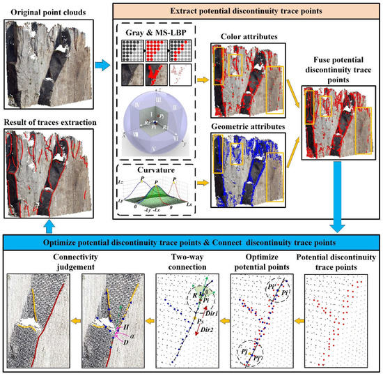
Figure 1.
The framework of the process of the proposed method.
2.1. Description of the Datasets
In this study, we used four datasets of 3D point clouds. The first dataset (example case) was used to explain the operating principle of the proposed method. The second dataset (Case A) contained data we collected in the field to verify the applicability of the proposed algorithm in real cases. The third dataset (Case B) was used to verify the applicability of the proposed algorithm in cases with a small number of point clouds and a large average spacing. The fourth dataset (Case C) was used to verify the applicability of the proposed algorithm in cases with a large number of point clouds and a small average spacing.
2.1.1. Example Case and Case B
Siefko Slob provided the raw data collected in Padua, Italy. The example case (Figure 2a) is a portion of the Case B data that was used to explain the operating principle of the proposed method. In the example case, the point cloud contained 37,879 points, the dimensions of the study area were 16.69 m × 13.63 m × 18.52 m and the average point spacing was 7.28 cm. In Case B (Figure 2c), the point cloud contained 125,230 points, the dimensions of the study area were 31.25 m × 41.88 m × 18.79 m and the average point spacing was 5.82 cm.
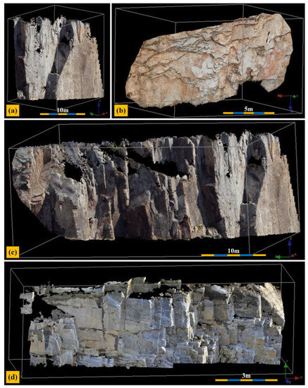
Figure 2.
Point cloud datasets. (a) Example case; (b) Case A; (c) Case B; (d) Case C.
2.1.2. Case A
The data for this case were real data we collected in the field. The study area is located on a slope along the Benxi Highway in Liaoning Province, China. A single-lens reflex (SLR) camera was used to obtain 44 images from three stations, and Agisoft PhotoScan software was used to extract a 3D point cloud from the slope (Figure 2b). For Case A, the point cloud contained 188,576 points, the dimensions of the study area were 12.22 m × 13.03 m × 8.39 m and the average point spacing was 2.23 cm. This study area is characterized by complex changes in the surface curvature of the rock mass.
2.1.3. Case C
The laser scanning data of Case C are open-source data, which can be obtained from Rockbench [7]. The study area for this case is near Ontario, Canada, and the original data were obtained with a Leica HDS6000 laser scanning system (Figure 2d). For Case C, the point cloud contained 2,170,033 points, the dimensions of the study area were 13.28 m × 4.21 m × 3.71 m and the average point spacing was approximately 5 mm. The point cloud in this case was characterized by a large number of high-density points.
2.2. Extraction of Potential Discontinuity Trace Points
This method is based on assessing both the color and geometric attributes of a 3D point cloud to extract a discontinuity trace. The potential discontinuity trace points are individually extracted from the color and geometric attributes of the 3D point cloud. Next, the two methods are fused to obtain more accurate discontinuity traces.
2.2.1. Extracting Potential Discontinuity Trace Points from the Color Attributes
Due to the influence of light, substantial changes in color typically occur at cracks on the surface of a rock mass and the turning points along the boundaries of the rock mass (Figure 3), which are reflected in the 3D point cloud. Accordingly, we used this feature to extract discontinuity trace points according to the color changes of the point cloud.
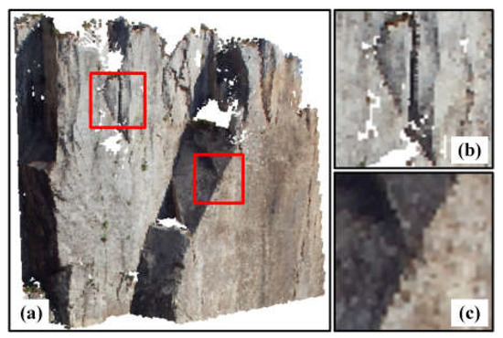
Figure 3.
3D point cloud of a rock mass. (a) Example case; (b) crack with a nonsignificant curvature change; (c) discontinuity trace with an obvious curvature change.
Step 1: Conversion of the color values to gray values. The color values represent the three colors (i.e., red, green and blue) of each point. In theory, we cannot numerically compare these three numbers. Therefore, we needed to convert the color values of the 3D point cloud to gray values to obtain a single gray value for each point. Here, we used the well-known psychological formula (luminance algorithm) [33]:
The grayscale model is shown in Figure 4b.
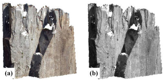
Figure 4.
Point cloud model. (a) Original color of the point cloud model; (b) grayscale model.
Step 2: Voxel segmentation. The number of point clouds was large, and their distribution was scattered, so the efficiency of processing all points would have been very low. Therefore, octree segmentation of the 3D point clouds in the study area was used here. In this process, all point clouds are divided into multiple cube units according to certain laws. Each cube unit becomes a voxel, then the color of each voxel is analyzed. Figure 5a–c shows the point clouds’ color changes in some voxels after segmentation. The point clouds in Figure 5b,c have no obvious color changes, while the point clouds in Figure 5a have obvious color changes, indicating that there are some discontinuity traces in these voxels. In the next step, we extracted the potential discontinuity trace points of these voxels.
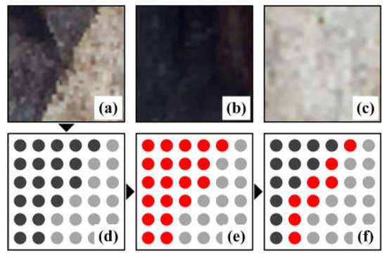
Figure 5.
Distribution of the 3D point cloud into voxels. (a–c) True color of the 3D point cloud on the surface of a rock mass in the voxels. (d) Sketch of the 3D point cloud. (e) Dark areas with substantial color changes (the red points). (f) Boundary of the dark areas (the red points).
Step 3: Extraction of potential discontinuity trace points. Statistical analysis was carried out on the voxels with obvious color changes, and it was found that the gray values of points in these voxels were distributed in a “hump-shaped” pattern, as shown in Figure 6. The first hump represents the area of the darker point cloud in the voxels, and the second hump represents the area of the lighter point cloud in the voxels. We needed to calculate the concave point between the two humps to divide the two areas. Here, the Otsu algorithm [34] was used to adaptively find the boundary value between the dark and light regions, that is, the green point in Figure 6. This concave point was set as the threshold to divide the depth of the voxel into two parts. If the color of a point in the divided voxel was less than this threshold, it was a dark area, which was recorded as a red point. After repeating this process, we obtained the red points in Figure 5e. Clearly, not all of the red points in this figure are discontinuity trace points. In the next step, we identified the boundary, and the red dots in Figure 5f were obtained.
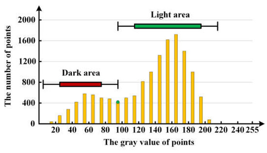
Figure 6.
Distribution of gray values of points in the voxels.
Step 4: Determination of light and shadow. As shown in Figure 7a, a light beam leaves shadows on the cracks and sheltered places on a rock mass’s surface. The cracks are effective discontinuity traces, and the shadow boundaries caused by occlusion are invalid. Therefore, we needed to eliminate invalid shadow boundaries.
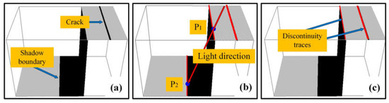
Figure 7.
Determination of shadows. (a) Crack and shadow boundary; (b) determining the direction of the illumination; (c) effective discontinuity traces (the black area is a shadow area, and are shadow points).
We considered different data collected at different places and different times. We needed to calculate the solar azimuth at different positions, including the solar altitude angle and the sun’s azimuth . The formulas are as follows:
where is the local latitude, is the solar declination and is the solar hour angle.
The direction of sunlight exposure can be calculated according to the solar altitude angle and the solar azimuth, as shown in Figure 7b. The sun will pass through and in turn. In this case, is a shadow point generated by the light and it is eliminated. After this step, we can obtain the effective discontinuity trace points, as shown in Figure 7c. Figure 8 shows the results of the actual test case.
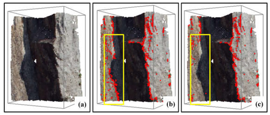
Figure 8.
The results of the actual test case. (a) Shadows from light; (b) potential discontinuity trace points extracted from the color attributes; (c) the result of introducing the light and shadow judgments.
Step 5: Multiscale space local binary patterns. When the geographic location and time of data acquisition are known, shadow points can be eliminated by the light and shadow judgments. However, many data are collected without recording the acquisition time, so it is impossible to calculate the direction of illumination. Other methods are needed to remove the shadow points. Therefore, a multiscale spatial local binary pattern (referred to as an MS-LBP) was proposed. As shown in Figure 9, this method eliminates the effect of illumination to some extent.
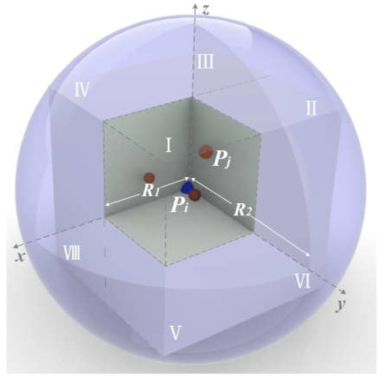
Figure 9.
MS-LBP schematic diagram. Ⅰ–Ⅷ represent the voxels in eight quadrants, where the blue sphere represents the detection point, the red spheres represent the internal points of each voxel, represents the side length of the voxel in each quadrant and represents the search radius in the neighborhood of the detection point.
Taking the detection point as the core, in the original point cloud coordinate system, the space is divided into eight quadrants with as the side length, and a 2 × 2 × 2 spatial cube is created. The voxels are denoted as Voxel I to Voxel VIII, as shown in Figure 9. To quickly retrieve a point from Voxel I to voxel VIII, a neighborhood search is established at detection point with a search radius of , where
That is, the smallest sphere can enclose eight voxels. We calculated the average gray value of all points in each voxel:
We calculated the MS-LBP value of each point. The average gray values of the eight voxels were compared with the gray value of the detection point. If a gray value was greater than the gray value of the detection point, the corresponding voxel was marked with a 1; otherwise, it was marked with a 0 (0 and 1 were used to resolve in Formula (7)). Thus, the 2 × 2 × 2 cube can produce an 8-bit binary number, which is converted into a decimal number in order from Voxel I to Voxel VIII, thus generating the MS-LBP value of the test point.
where
The MS-LBP models obtained at different scales are shown in Figure 10.
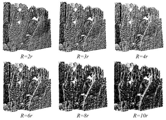
Figure 10.
MS-LBP models at different scales (r is the average spacing of the original point cloud).
Finally, the redundant points among the potential discontinuity trace were removed with the MS-LBP model, as shown in Figure 11b.
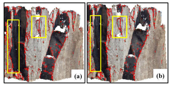
Figure 11.
Diagram of discontinuity trace points. (a) The result without the MS-LBP constraint; (b) the result of adding the MS-LBP constraint.
2.2.2. Extracting the Potential Discontinuity Trace Points from the Geometric Attributes
The geometric attributes of the point cloud characterize the spatial relationships of the discontinuity traces on the surface of the rock mass. These discontinuity traces include valley lines, ridge lines and cracks. The valley lines and ridge lines are areas where the curvature changes greatly. We can obtain these lines through a transformation of the curvature. Here, we used a Fourier series to calculate the curvature at each point of the 3D point cloud to obtain the potential ridge points and valley points [1].
2.3. Optimization of Potential Discontinuity Trace Points
Both the potential discontinuity trace points extracted from the color attributes of the 3D point cloud and the potential ridge points and valley points extracted from the geometric attributes were relatively scattered. Hence, these points needed to be further optimized to obtain the final discontinuity trace points.
This study proposed a new local point straight-line normalization smoothing algorithm. A diagram of the operating principle of this algorithm is shown in Figure 12. The basic operating principle is as follows:
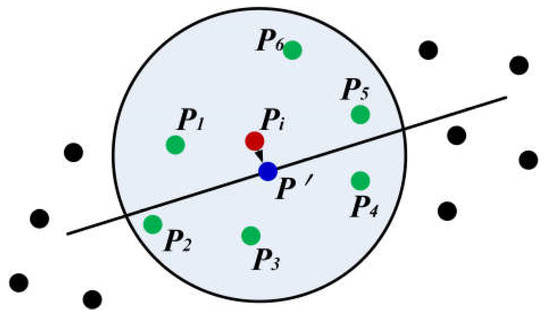
Figure 12.
Diagram of the operating principle of the local point straight-line normalization smoothing algorithm (the black points, the green points and the red point are the points before smoothing, and the blue point is the point after smoothing).
Step 1: Perform neighborhood radius searches for each point and save all points in the neighborhood to a point list.
Step 2: Fit all points in the point list to a straight line. Here, principal component analysis is used to fit a straight line in space. The direction vector of the fitted line and a point on the line are calculated, then the fitted straight line L is expressed as follows:
Step 3: Move the query point to the fitted straight line, i.e., project point onto the fitted straight line to obtain .
Determine a level according to the query point and the straight line L:
According to Formula (6), we can obtain the following expressions:
By substituting Formula (8) into Formula (7), the linear parameter t can be obtained. By substituting t into Formula (6), the projection point can be obtained.
Step 4: Repeat Steps 1 to 3 and obtain the discontinuity trace points after optimization, which are shown in blue in Figure 13. The red and black points in this figure are the discontinuity trace points before optimization.
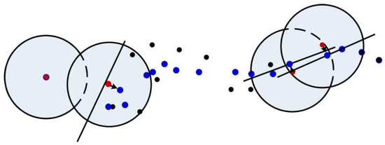
Figure 13.
Diagram of the normalized smoothing process of the local straight line of the potential discontinuity trace points (the black points and red points are the points before smoothing, and the blue points are the points after smoothing).
2.4. Connecting the Discontinuity Trace Points
When connecting discontinuity traces by a traditional region-growing algorithm [1], the connection effect is often unsatisfactory and there will be problems such as discontinuity trace segment connections, line segment cross-connection errors and unconnected cross-points, as shown in Figure 14a. The reason for these issues is that a traditional region-growing algorithm can only make a one-way connection and cannot effectively determine the direction of the line segment when it encounters an intersection. To address this, we proposed a two-way connection algorithm for establishing a local vector buffer. A diagram of this two-way algorithm is shown in Figure 15. The basic operating principle of this algorithm is as follows:
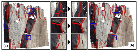
Figure 14.
Comparison with existing methods. (a) A traditional region-growing connection algorithm; (b) the proposed algorithm.
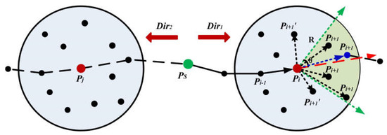
Figure 15.
Diagram of the algorithm for establishing a two-way connection for a local vector buffer. The green point is any starting point, the red points are the current search points, the black points are the search points in the neighborhood, the blue point is the next connection point, the red line is the trend of the current trace, the angle θ between the two green lines is the direction threshold, and the search radius is R.
Step 1: Take any point as the starting point. First, make a one-way connection, assuming the direction is . If a cross-branch point is encountered during the connection process, create a local buffer at . Hence, a nearest neighbor search must be performed for the point , where is the previous connection point. is the nearest point searched.
Step 2: Calculate the direction of the connected trace , namely the direction of the red line in Figure 15, where:
Calculate the direction from the search point to all neighborhood points, that is, the direction of the black dotted line in Figure 15, where:
Calculate the angle between two directions , where:
If the direction is greater than threshold , as is the case for point in Figure 15, the point will not be connected. If the direction is less than threshold , as is the case for point in Figure 15, the connection weight coefficients of the adjacent points that meet the conditions are calculated.
Step 3: Calculate the connection weight coefficient, referred to as the CWC, with the following formula
where is the Euclidean distance between the adjacent point and search point , and is the angle included between and . The smaller the CWC is, the better this point meets the connection conditions, and it is the next optimal connection point; an example is the blue point in Figure 15. Different neighborhood radius thresholds and direction thresholds produce different results. Therefore, we performed a comparative analysis of the experimental results under different thresholds, as shown in Figure 16. The effect was best when the neighborhood radius is 6r and the direction threshold is 25, where r is the average spacing of the original point cloud. Steps 1 to 3 are repeated until the one-way search is completed.
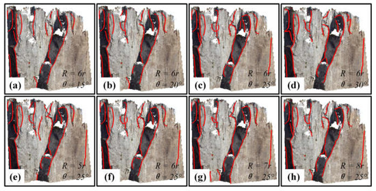
Figure 16.
Comparison of different neighborhood radius thresholds and direction thresholds. (a–d) Results of different angle thresholds; (e–h) results of different neighborhood radius thresholds.
Step 4: Make a reverse connection at the starting point ; that is, repeat Steps 1 to 3 in the direction of until the reverse search is also completed and all points have been traversed.
Step 5: Connectivity judgment [29]. Perform a proximity search of the distance D at the endpoint () of any discontinuity trace (such as the blue line in Figure 17) to search for adjacent discontinuity traces (such as the black line and green line in Figure 17). Calculate and determine the trend of the connected discontinuity trace and the trend of the adjacent discontinuity trace . The reason why the 1/3 inverse is used to represent the trend of the discontinuity trace is that it is too short to reflect the local trend of the discontinuity trace. If the length is too great, it over-reflects the local trend of the discontinuity trace. If the direction offset is less than , the spatial offset is determined. Calculate the spatial offset of the remaining adjacent discontinuity trace and the detected discontinuity trace that meet the determined distance and the determined direction offset; that is, calculate the spatial distance between them. If this distance is less than H, it is the optimal connecting discontinuity trace (the green line in Figure 17) and it is connected to the detected discontinuity trace. The final result of the connectivity judgment is shown in Figure 14b.
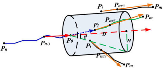
Figure 17.
Diagram of connectivity judgments. The blue line is the connected discontinuity trace, the red arrows indicate the connected discontinuity trace, the black line is near the discontinuity trace, the orange arrows indicate locations maintaining a connection to the discontinuity trace, the green line is the best connected discontinuity trace, D is the connection radius, is the directional offset and H is the spatial offset.
2.5. Calculation of the Area Density
The density of the discontinuity traces of a rock mass generally falls into one of three categories: line density, area density or bulk density. The area density is the best tool for quantifying the degree of fracture development in a specific area. In this study, the discontinuity traces were projected onto a plane perpendicular to the normal vector of the overall point cloud. The formula of the area density is as follows:
where is the length of each trace and S is the projected area.
3. Case Studies
According to the proposed overall process, we developed a prototype system based on the Qt and C++ programming languages. Three experimental cases were used to compare the proposed method with existing methods to verify the applicability of our method.
3.1. Case A: Overall Process Analysis and Comparison
Figure 18a shows the potential discontinuity trace points extracted from the color attributes of the point cloud. Figure 18b shows the optimization of the potential discontinuity trace points using the local straight-line normalization smoothing algorithm presented in this article. The results show that the optimized discontinuity trace points can clearly represent the distribution and direction of the discontinuity traces. Figure 18c shows the discontinuity traces obtained after the points were connected using a traditional region-growing algorithm. There are many problems with the discontinuity of the line segments’ connection. Figure 18d shows the discontinuity traces obtained after establishing connections through the connection algorithm using a two-way local vector buffer. It can be clearly seen that the proposed method can effectively connect the discontinuity traces. Figure 18e shows the discontinuity traces extracted from the geometric attributes alone [1]. Figure 18f shows the discontinuity traces extracted from the combination of the color and the geometric attributes. A comparative analysis shows that if the curvature change of the point cloud of the surface of the rock mass is small or the change is more complex, the discontinuity traces extracted from the geometric attributes alone will be more scattered and insufficiently accurate (Figure 18e). The discontinuity traces extracted from the color attributes will compensate for this defect, and the combination of the color and the geometric attributes will make the discontinuity traces more accurate and reliable (Figure 18f).
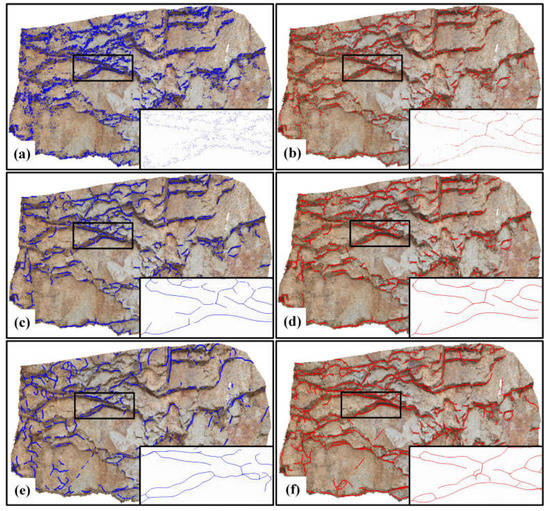
Figure 18.
Case A: Overall process of analysis and comparison. (a) Potential discontinuity trace points extracted from the color attributes; (b) discontinuity trace points optimized using the local straight-line normalization smoothing algorithm; (c) discontinuity traces connected using the traditional region-growing algorithm and the connectivity judgment algorithm; (d) discontinuity traces connected using the proposed connection algorithm; (e) discontinuity traces extracted from the geometric attributes; (f) the results of fusing the color and geometric attributes.
3.2. Case B: Comparison of the Results of the Proposed Method with Those of Existing Methods
Case B is a dataset that is greatly affected by sunlight, as shown in Figure 19. The proposed method could still extract ideal discontinuity traces based on the combination of color and geometric attributes. These results were compared with the discontinuity traces extracted using the tensor voting algorithm [32] (such as in Figure 19a). Here, cracks with no obvious fluctuation on the rocks’ surface could be obtained. However, due to the greater influence of sunlight, some more obvious shadow boundaries could also be mistaken for traces and extracted (Figure 19b). After applying the illumination analysis and MS-LBP constraint, these redundant discontinuity traces were effectively eliminated (Figure 19c).
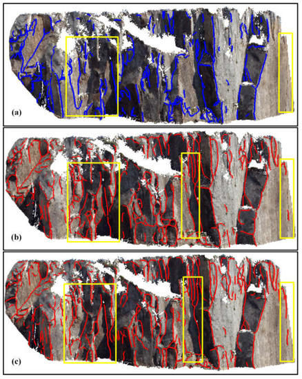
Figure 19.
Case B: Comparison of the proposed method and existing methods. (a) The discontinuity traces extracted using tensor voting; (b) the result of fusing color and the geometric attributes; (c) the result of removing shadows by determining the light and shadow and the MS-LBP constraint.
3.3. Case C: Comparison of the Results of the Proposed Method with Those of Existing Methods
Case C is a dataset with a large amount of point cloud data and high point cloud density. This dataset has been used by many researchers [1,2,4,5,6,7]. Here, we used this dataset for a comparison with existing research methods [2,32]. Image processing technology was used to extract the discontinuity traces (Figure 20a). The problem with this approach is that the extraction process is cumbersome, and the discontinuity traces in the image are detected and extracted by several related software packages. Many manual interactions were needed, and the final trace connection was trivial (Figure 20d). The discontinuity traces were also extracted using tensor voting (Figure 20b). The problem with this method is that tensor voting can clearly extract sharp parts, but it cannot extract certain cracks (Figure 20e). To solve these problems, we used the combination of the color and the geometric attributes of the 3D point cloud of the rock mass to extract the discontinuity trace points and connect them through the proposed connection algorithm (Figure 20c). This approach could extract discontinuity traces with small curvature changes while maintaining a high degree of automation. Moreover, the proposed method produced ideal extraction results (Figure 20f).
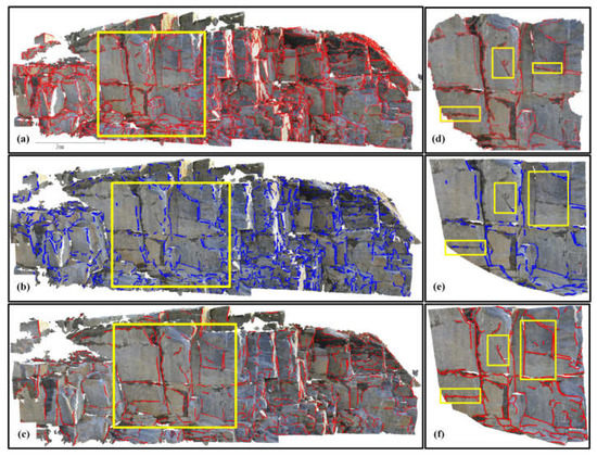
Figure 20.
Case C: Comparison between the proposed method and existing methods. (a) Discontinuity traces extracted using only texture attributes; (b) discontinuity traces extracted using tensor voting and geometric attributes; (c) discontinuity traces extracted using the proposed method with both geometric and color attributes; (d–f) detailed results of the different methods.
3.4. Calculation of the Area Density and the Average Discontinuity Trace Length
In this study, the area density of the rock mass and average discontinuity trace lengths of the three cases were calculated and compared with those of existing methods. The proposed method addressed the defects of the existing methods when extracting discontinuity traces, as shown in Table 1.

Table 1.
Area density and average discontinuity track length of the rock mass.
4. Discussion
There are two ways to extract the discontinuity traces of a rock mass. One is to extract them through image recognition technology. Because a photo image is 2D data, the occlusion problem in a 3D scene is difficult to address, and the identified discontinuity traces are not sufficiently accurate. The second method is to extract the discontinuity traces by calculating the curvature of each point from the geometric attributes of a 3D point cloud. In this way, only discontinuity traces with obvious curvature changes will be extracted. It is difficult to identify cracks on the plane. In this study, discontinuity traces were extracted by directly analyzing the color attributes of the original 3D point cloud. This made full use of the color attributes often ignored in 3D point cloud data. By fusing these results with the geometric attributes of the point cloud, the discontinuity traces could be extracted more accurately.
The actual collected color attributes of a rock mass’s surface will produce shadows under the influence of light. The influence of light on the rock mass’s surface shadows is also different in different geographical locations and at different acquisition times. When the location and time of data acquisition are known, we can eliminate the influence of shadows by calculating the solar altitude and solar azimuth. However, some data are collected without recording the specific time, so it is impossible to accurately calculate the lighting direction in this way to eliminate the influence of shadows. Therefore, we proposed an MS-LBP algorithm to eliminate the influence of shadows. This method of eliminating shadows is not as effective as directly calculating the direction of illumination. However, it is feasible to use this method when the geographical locations and acquisition times of the data are not known.
For connecting discontinuity trace points, we proposed a new connection algorithm by establishing the two-way connections of a local vector buffer and making a connectivity judgment. This algorithm can effectively solve the problems of crossover, overlap, turnback, discontinuity and so on. However, this method requires relevant parameters to be set. There are five important parameters involved, including two connection parameters (the search radius R and the direction threshold ) and three connectivity judgment parameters (the connection radius D, the direction offset and the spatial offset H). Different parameter settings will have a certain impact on the results. Figure 15 shows different results with different parameter settings. The ranges of parameter settings and the best values are shown in Table 2.
Table 2.
Parameter settings for connecting discontinuity traces.
Although the proposed method could effectively extract the discontinuity traces of a rock mass’s surface, there are still some problems worth studying in the future. For example, we could not accurately distinguish between natural traces and artificial traces. It is difficult to distinguish these two types of traces by sight, and it is even more difficult for us to process them by using a computer. We have not found a suitable method to address this issue. We aim to find solutions through machine learning if possible.
5. Conclusions
In this study, a new method for the automatic extraction and connection of discontinuity traces on rock surfaces based on 3D point clouds was proposed. The color and geometric attributes of the original 3D point clouds were combined to extract potential discontinuity trace points. Some discontinuity traces on a smooth rock surface can be extracted by directly analyzing the color attributes of the 3D point clouds, which can effectively compensate for the incomplete extraction of discontinuity traces using only the geometric attributes of the point clouds. Shadows produced by illumination have a certain impact on the results. To eliminate the influence of illumination, the geographical location and acquisition time of the data are fully considered. However, some data do not contain the geographical location and collection time of when they were collected. The proposed MS-LBP algorithm can effectively eliminate the shadow points caused by illumination. For connecting discontinuity traces, we proposed an algorithm for establishing the two-way connections of a local vector buffer and obtaining a connectivity judgment. Compared with a traditional growth connection algorithm, this method could more effectively solve the problems of intersection, overlap, turnback, discontinuity and so on. At the same time, through incorporation of the results of extracting the discontinuity traces, the area density of a rock mass can be calculated, which can provide some data support for the stability of rock slopes.
In addition, we developed a prototype system for extracting the discontinuity traces of rock masses. It has a high degree of automation, does not require large-scale human interaction and can greatly improve the efficiency of work.
Author Contributions
J.G. and Z.Z. conceived the manuscript; Z.Z. addressed the 3D point cloud data; Z.Z. was responsible for the research method; J.G. provided funding support and ideas; J.G., Z.Z., Y.M., S.L., W.Z. and T.Y. helped to improve the manuscript. All authors have read and agreed to the published version of the manuscript.
Funding
The work was funded by the National Natural Science Foundation of China (grant numbers 42172327 and 41671404] and the Fundamental Research Funds for the Central Universities (grant number N2201022).
Data Availability Statement
The original data of the three cases and the program codes of the proposed method of extracting discontinuity traces are available from the corresponding author upon reasonable request.
Acknowledgments
We are very grateful to the editors and four anonymous reviewers for their insightful comments and suggestions, which led to the improvement of the manuscript.
Conflicts of Interest
The authors declare no conflict of interest.
References
- Guo, J.T.; Wu, L.X.; Zhang, M.M.; Liu, S.J.; Sun, X.Y. Towards automatic discontinuity trace extraction from rock mass point cloud without triangulation. Int. J. Rock Mech. Min. Sci. 2018, 112, 226–237. [Google Scholar] [CrossRef]
- Guo, J.T.; Liu, Y.H.; Wu, L.X.; Liu, S.J.; Yang, T.H.; Zhu, W.C.; Zhang, Z.R. A geometry- and texture-based automatic discontinuity trace extraction method for rock mass point cloud. Int. J. Rock Mech. Min. Sci. 2019, 124, 104132. [Google Scholar] [CrossRef]
- Zhang, W.; Lan, Z.G.; Ma, Z.F.; Tan, C.; Que, J.S.; Wang, F.Y.; Cao, C. Determination of statistical discontinuity persistence for a rock mass characterized by non-persistent fractures. Int. J. Rock Mech. Min. Sci. 2020, 126, 104177. [Google Scholar] [CrossRef]
- Riquelme, A.J.; Abelian, A.; Tomas, R. Discontinuity spacing analysis in rock masses using 3D point clouds. Eng. Geol. 2015, 195, 185–195. [Google Scholar] [CrossRef]
- Ge, Y.F.; Cao, B.; Tang, H.M. Rock Discontinuities Identification from 3D Point Clouds Using Artificial Neural Network. Rock Mech. Rock Eng. 2022, 55, 1705–1720. [Google Scholar] [CrossRef]
- Guo, J.T.; Liu, S.J.; Zhang, P.N.; Wu, L.X.; Zhou, W.H.; Yu, Y.N. Towards semi-automatic rock mass discontinuity orientation and set analysis from 3D point clouds. Comput. Geosci. 2017, 103, 164–172. [Google Scholar] [CrossRef]
- Lato, M.; Kemeny, J.; Harrap, R.M.; Bevan, G. Rock bench: Establishing a common repository and standards for assessing rockmass characteristics using LiDAR and photogrammetry. Comput. Geosci. 2013, 50, 106–114. [Google Scholar] [CrossRef]
- Chen, N.; Kemeny, J.; Jiang, Q.H.; Pan, Z.W. Automatic extraction of blocks from 3D point clouds of fractured rock. Comput. Geosci. 2017, 109, 149–161. [Google Scholar] [CrossRef]
- Weidner, L.; Walton, G.; Kromer, R. Classification methods for point clouds in rock slope monitoring: A novel machine learning approach and comparative analysis. Eng. Geol. 2019, 263, 105326. [Google Scholar] [CrossRef]
- Riquelme, A.J.; Tomas, R.; Abellan, A. Characterization of rock slopes through slope mass rating using 3D point clouds. Int. J. Rock Mech. Min. Sci. 2016, 84, 165–176. [Google Scholar] [CrossRef]
- Wang, S.H.; Ni, P.P.; Guo, M.D. Spatial characterization of joint planes and stability analysis of tunnel blocks. Tunn. Undergr. Space Technol. 2013, 38, 357–367. [Google Scholar] [CrossRef]
- Acharya, B.; Sarkar, K.; Singh, A.K.; Chawla, S. Preliminary slope stability analysis and discontinuities driven susceptibility zonation along a crucial highway corridor in higher Himalaya, India. J. Mt. Sci. 2020, 17, 801–823. [Google Scholar] [CrossRef]
- Zhang, Q.; Wang, Q.; Chen, J.P.; Li, Y.Y.; Ruan, Y.K. Estimation of mean trace length by setting scanlines in rectangular sampling window. Int. J. Rock Mech. Min. Sci. 2016, 84, 74–79. [Google Scholar] [CrossRef]
- Menegoni, N.; Giordan, D.; Perotti, C.; Tannant, D.D. Detection and geometric characterization of rock mass discontinuities using a 3D high-resolution digital outcrop model generated from RPAS imagery—Ormea rock slope, Italy. Eng. Geol. 2019, 252, 145–163. [Google Scholar] [CrossRef]
- Nesbit, P.R.; Durkin, P.R.; Hugenholtz, C.H.; Hubbard, S.M.; Kucharczyk, M. 3-D stratigraphic mapping using a digital outcrop model derived from UAV images and structure-from-motion photogrammetry. Geosphere 2018, 14, 2469–2486. [Google Scholar] [CrossRef]
- Chesley, J.T.; Leier, A.L.; White, S.; Torres, R. Using unmanned aerial vehicles and structure-from-motion photogrammetry to characterize sedimentary outcrops: An example from the Morrison Formation, Utah, USA. Sediment. Geol. 2017, 354, 1–8. [Google Scholar] [CrossRef]
- Roncella, R.; Forlani, G.; Remondino, F. Photogrammetry for geological applications: Automatic retrieval of discontinuity orientation in rock slopes. Conf. Videometrics VIII 2005, 5665, 17–27. [Google Scholar]
- Corradetti, A.; McCaffrey, K.; De Paola, N.; Tavani, S. Evaluating roughness scaling properties of natural active fault surfaces by means of multi-view photogrammetry. Tectonophysics 2017, 717, 599–606. [Google Scholar] [CrossRef]
- Gigli, G.; Casagli, N. Semi-automatic extraction of rock mass structural data from high resolution LIDAR point clouds. Int. J. Rock Mech. Min. Sci. 2011, 48, 187–198. [Google Scholar] [CrossRef]
- Fisher, J.E.; Shakoor, A.; Watts, C.F. Comparing discontinuity orientation data collected by terrestrial LiDAR and transit compass methods. Eng. Geol. 2014, 181, 78–92. [Google Scholar] [CrossRef]
- Caudal, P.; Grenon, M.; Turmel, D.; Locat, J. Analysis of a Large Rock Slope Failure on the East Wall of the LAB Chrysotile Mine in Canada: LiDAR Monitoring and Displacement Analyses. Rock Mech. Rock Eng. 2017, 50, 807–824. [Google Scholar] [CrossRef]
- Pagano, M.; Palma, B.; Ruocco, A.; Parise, M. Discontinuity Characterization of Rock Masses through Terrestrial Laser Scanner and Unmanned Aerial Vehicle Techniques Aimed at Slope Stability Assessment. Appl. Sci.-Basel 2020, 10, 2960. [Google Scholar] [CrossRef]
- Cao, T.; Xiao, A.C.; Wu, L.; Mao, L.G. Automatic fracture detection based on Terrestrial Laser Scanning data: A new method and case study. Comput. Geosci. 2017, 106, 209–216. [Google Scholar] [CrossRef]
- Cheng, L.; Tong, L.H.; Li, M.C.; Liu, Y.X. Semi-Automatic Registration of Airborne and Terrestrial Laser Scanning Data Using Building Corner Matching with Boundaries as Reliability Check. Remote Sens. 2013, 5, 6260–6283. [Google Scholar] [CrossRef]
- Battulwar, R.; Zare-Naghadehi, M.; Emami, E.; Sattarvand, J. A state-of-the-art review of automated extraction of rock mass discontinuity characteristics using three-dimensional surface models. J. Rock Mech. Geotech. Eng. 2021, 13, 920–936. [Google Scholar] [CrossRef]
- Kemeny, J.; Post, R. Estimating three-dimensional rock discontinuity orientation from digital images of fracture traces. Comput. Geosci. 2003, 29, 65–77. [Google Scholar] [CrossRef]
- Lemy, F.; Hadjigeorgiou, J. Discontinuity trace map construction using photographs of rock exposures. Int. J. Rock Mech. Min. Sci. 2003, 40, 903–917. [Google Scholar] [CrossRef]
- Umili, G.; Ferrero, A.; Einstein, H.H. A new method for automatic discontinuity traces sampling on rock mass 3D model. Comput. Geosci. 2013, 51, 182–192. [Google Scholar] [CrossRef]
- Kong, D.H.; Wu, F.Q.; Saroglou, C. Automatic identification and characterization of discontinuities in rock masses from 3D point clouds. Eng. Geol. 2019, 265, 105442. [Google Scholar] [CrossRef]
- Ge, Y.F.; Tang, H.M.; Xia, D.; Wang, L.Q.; Zhao, B.B.; Teaway, J.W.; Chen, H.Z.; Zhou, T. Automated measurements of discontinuity geometric properties from a 3D-point cloud based on a modified region growing algorithm. Eng. Geol. 2018, 242, 44–54. [Google Scholar] [CrossRef]
- Li, X.J.; Chen, J.Q.; Zhu, H.H. A new method for automated discontinuity trace mapping on rock mass 3D surface model. Comput. Geosci. 2016, 89, 118–131. [Google Scholar] [CrossRef]
- Zhang, K.S.; Wu, W.; Zhu, H.H.; Zhang, L.Y.; Li, X.J.; Zhang, H. A modified method of discontinuity trace mapping using three-dimensional point clouds of rock mass surfaces. J. Rock Mech. Geotech. Eng. 2020, 12, 571–586. [Google Scholar] [CrossRef]
- Burger, W.; Burge, M.J. Digital Image Processing; Springer: Cham, Switzerland, 2022; pp. 387–388. [Google Scholar]
- Otsu, N. Threshold selection method from gray-level historams. Ieee Trans. Syst. Man Cybern. 1979, 9, 62–66. [Google Scholar] [CrossRef]


Publisher’s Note: MDPI stays neutral with regard to jurisdictional claims in published maps and institutional affiliations. |
© 2022 by the authors. Licensee MDPI, Basel, Switzerland. This article is an open access article distributed under the terms and conditions of the Creative Commons Attribution (CC BY) license (https://creativecommons.org/licenses/by/4.0/).