Article

Convolutional Neural Network Chemometrics for Rock Identification Based on Laser-Induced Breakdown Spectroscopy Data in Tianwen-1 Pre-Flight Experiments

1
Key Laboratory of Space Active Opto-Electronics Technology, Shanghai Institute of Technical Physics, Chinese Academy of Sciences, Shanghai 200083, China
2
School of Physics and Optoelectronic Engineering, Hangzhou Institute for Advanced Study, University of Chinese Academy of Sciences, Hangzhou 310024, China
3
Department of Remote Sensing and Photogrammetry, Finnish Geospatial Research Institute, 02430 Kirkkonummi, Finland
*
Author to whom correspondence should be addressed.
Remote Sens. 2022, 14(21), 5343; https://doi.org/10.3390/rs14215343
Submission received: 23 August 2022 / Revised: 9 October 2022 / Accepted: 22 October 2022 / Published: 25 October 2022

Abstract

:
Laser-induced breakdown spectroscopy (LIBS) coupled with chemometrics is an efficient method for rock identification and classification, which has considerable potential in planetary geology. A great challenge facing the LIBS community is the difficulty to accurately discriminate rocks with close chemical compositions. A convolutional neural network (CNN) model has been designed in this study to identify twelve types of rock, among which some rocks have similar compositions. Both the training set and the testing set are constructed based on the LIBS spectra acquired by Mars Surface Composition Detector (MarSCoDe) for China’s Tianwen-1 Mars exploration mission. All the spectra were collected from dedicated rock pellet samples, which were placed in a simulated Martian atmospheric environment. The classification performance of the CNN has been compared with that of three alternative machine learning algorithms, i.e., logistic regression (LR), support vector machine (SVM), and linear discriminant analysis (LDA). Among the four methods, it is on the CNN model that the highest classification correct rate has been obtained, as assessed by precision score, recall score, and the harmonic mean of precision and recall. Furthermore, the classification accuracy is inspected more quantitatively via Brier score, and the CNN is still the best performing model. The results demonstrate that the CNN-based chemometrics are an efficient tool for rock identification with LIBS spectra collected in a simulated Martian environment. Despite the relatively small sample set, this study implies that CNN-supported LIBS classification is a promising analytical technique for Tianwen-1 Mars mission and more planetary explorations in the future.

1. Introduction

Laser-induced breakdown spectroscopy (LIBS) is a technique in which high-power-density laser pulses are focused onto a tiny area of a target and the induced plasma emission is collected by spectrometers [1]. LIBS is well known as a versatile approach to carry out chemical composition analysis, since the characteristic emission lines in a LIBS spectrum can be employed as “fingerprints” to identify the chemical elements contained in the target sample [2]. LIBS has the advantage of implementing in situ and stand-off detection, and it has been extensively applied in various fields, such as biomedicine [3], the metallurgical industry [4], environmental monitoring [5], energy science [6], nuclear security [7], geological investigation [8,9], etc. Particularly, the remote detection capability of LIBS has made it an outstanding tool for space exploration.
NASA’s Curiosity rover carried a LIBS instrument named ChemCam in Mars Science Laboratory (MSL) mission, marking the first LIBS application in planetary exploration [10,11,12]. Arriving on Mars within Curiosity in 2012, ChemCam has carried out chemical composition investigation of rocks and soils on Martian surface [13,14,15,16,17]. Moreover, NASA’s Perseverance rover is equipped with an upgraded LIBS suite, called SuperCam, in Mars 2020 mission [18,19,20,21]. Recently the results of major element quantification based on the LIBS spectra collected by SuperCam have been reported by Anderson et al. [22].
China’s first Mars exploration, i.e., Tianwen-1 mission, was launched in July 2020. The Tianwen-1 lander touched down on Mars in May 2021 with a Mars rover called Zhurong (the name of the God of Fire in ancient Chinese mythology). Similar to Curiosity and Perseverance, Zhurong rover also carries a LIBS instrument entitled MarSCoDe, standing for Mars Surface Composition Detector [23]. MarSCoDe will carry out a series of geochemical investigations, among which, one of the important tasks is to identify the various types of rocks on Martian surface.
LIBS technique is a good tool to perform stand-off detection and realize efficient identification of target rocks in planetary geology studies [24]. Of course, it is noteworthy that appropriate chemometrics also play an essential role in LIBS analysis. Nowadays LIBS chemometrics based on machine learning have been widely used in sample classification. Yang et al. achieved an over 90% average correct rate in classification of six classes of rock samples and seven classes of soil samples, by two multivariate analysis methods, i.e., partial least squares discriminant analysis (PLS-DA) and support vector machine (SVM) [25]. Vítková et al. fed a linear discriminant analysis (LDA) model and an artificial neural network (ANN) with the principal components of LIBS spectra, respectively [26]. The LDA correctly classified six out of the eight kinds of materials, while the ANN overperformed with seven successful cases. Yelameli et al. tried k-nearest neighbor (KNN), ANN, and SVM to classify 30 different rock samples, respectively, and the SVM algorithm performed the best with an accuracy of better than 95% [27]. Bi et al. figured out that the accuracy of mineral classification could be improved by exploiting joint LIBS-Raman spectra data, regardless of their concrete classification algorithm (ANN, PLS-DA, or SVM) [28].
Particularly in recent studies, ANN algorithms have been extensively adopted in LIBS spectra data analysis [29,30]. As one of the most popular ANN algorithms, convolutional neural network (CNN) has received considerable interest in spectroscopic analysis researches [31,32]. Nevertheless, CNN has not been valued in LIBS studies until very recently. As a pioneering work, Lu et al. analyzed time-resolved LIBS spectra by a CNN to improve potassium detection accuracy in soil samples [33]. The CNN in their work comprises only one convolutional layer and one pooling layer, so it is a so-called shallow network. As a matter of fact, a CNN uses convolution layers to extract features and pooling layers to reduce parameter quantity and hence prevent over-fitting. Therefore, a CNN containing more layers, i.e., a deep network, is routinely more competent for deep learning and accurate analysis. Deep CNNs have been proven to have excellent capability in classification and recognition [34,35]. Specifically for LIBS analysis, our group has demonstrated that a deep CNN can be employed for multi-component quantitative analysis upon rock and soil samples, and outshines PLS and back-propagation neural network in terms of overall accuracy [36]; and very recently we have also utilized the CNN-LIBS method to address the issue of sampling distance effect in geochemical sample classification [37].
This study constructs a deep CNN to conduct rock classification, based on the LIBS spectra acquired by MarSCoDe in Tianwen-1 pre-flight experiments. The target samples for these experiments were twelve types of rocks in the form of pellets, which were placed in a simulated Martian atmospheric environment during the measurements. Besides the CNN, three alternative machine learning methods for classification, including logistic regression (LR), SVM, and LDA, have also been evaluated, and the classification performance of the four methods are compared. The results show that the proposed deep CNN can outperform the other three classical machine learning techniques, indicating that the CNN classification model integrated with the MarSCoDe LIBS technology can be a promising methodology for investigating the geology of the Tianwen-1 landing site.
The rest of this paper is organized as follows: Section 2 introduces Tianwen-1 mission background and the methods in this study, including the experimental setup and the machine learning models; Section 3 presents the results and provides some discussion; Section 4 makes a concise conclusion.

2. Background and Methods

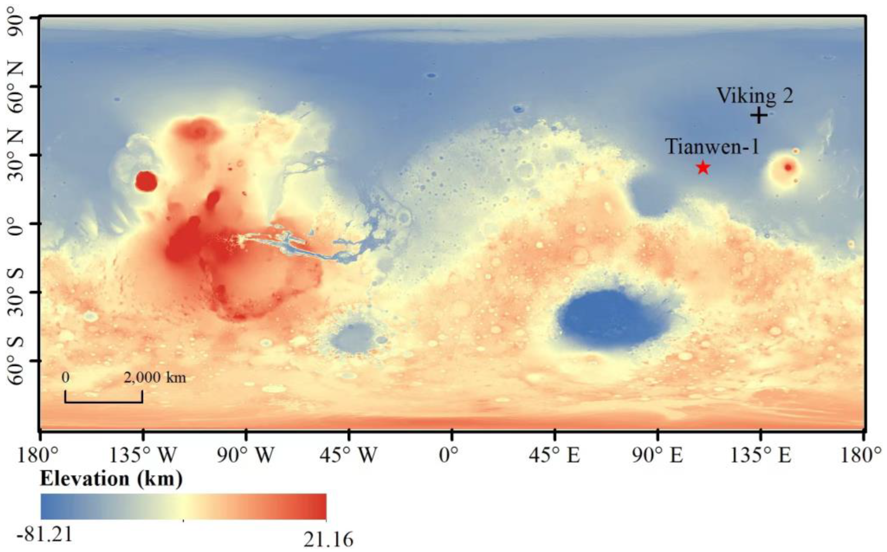
2.1. Mission Background and Scientific Goals

Zhurong rover consists of six major payloads, besides MarSCoDe, there are also Multispectral Camera, Terrain Camera, Mars-Rover Subsurface Exploration Radar, Mars Magnetic Field Detector, and Mars Meteorology Monitor [38]. These payloads are expected to help achieve the scientific goals of Tianwen-1 mission, i.e., (1) to characterize the Martian morphology and geological structure; (2) to investigate the soil features and water-ice distribution; (3) to detect the chemical composition of the Martian surface; (4) to study the atmosphere ionosphere and surface climate of Mars; and (5) to explore the physical field and internal structure of Mars. The MarSCoDe instrument is mainly responsible for the third scientific goal.
The landing site of Zhurong rover is Utopia Planitia, a large plain centered at 46.7°N, 117.5°E [39], as illustrated in Figure 1. Utopia Planitia has undergone extensive resurfacing and infilling processes, e.g., continuing volcanism from Elysium has filled most of the Utopia Planitia area with lava and eruption materials [40]. Landforms, such as polygons and scalloped depressions, have been observed in the area [41], and the existence of a meter-thick mantle possibly containing an ice–dust admixture has been reported [42,43,44]. Although orbital remote sensors have not found extensive hydrated mineral exposed in this area, in situ detection (e.g., LIBS) is likely to obtain the evidence for water activity in ancient times, and the results may provide significant constraints on the ocean hypothesis on the northern lowland area and the evolution of global climate.

2.2. LIBS Experiments and Data Preprocessing

Carried by Zhurong rover, the MarSCoDe instrument can implement LIBS detection after the landing, as illustrated in Figure 2. The technical specifications of MarSCoDe LIBS system are listed in Table 1.
Figure 3 displays the diagram of the LIBS experimental setup, including the MarSCoDe instrument and the Martian atmosphere simulation chamber holding the rock samples. The excitation source is a high-power Nd: YAG 1064 nm laser, with the pulse width of approximately 4 ns and the pulse energy up to 9 mJ. The repetition rate was set to 3 Hz in this experiment. The whole spectrometer system includes three 1800-pixel spectral channels, which are actually three spectrometers covering three bands, i.e., 240–340 nm, 340–540 nm, and 540–850 nm, respectively. The radiation of the laser-induced plasma is collected by a coaxial Cassegrain telescope and imported into the three spectrometers through fibers. There is a main controller which steers the optical system, enabling the laser to exactly point the target sample. The controller is also in charge of spectra data transmission, with 5400 data points included in each captured LIBS spectrum.
The experiment in this study employed 12 different types of rocks, including (1) andesite, (2) dolomite, (3) opal, (4) kaolinite, (5) potash feldspar, (6) montmorillonite, (7) diopside, (8) basalt, (9) hematite, (10) olivine, (11) albite, and (12) gypsum. Each type of rock was ground into powder particles with a less than 37 μm diameter and pressed into cylindrical pellets with a radius of 20 mm. These rocks were selected since they are common sedimentary rocks or igneous rocks which contain the elements most likely to exist on Mars, such as Si, Fe, Mg, Al, Ca, and K [45,46]. Some of the sample pellets are exhibited in Figure 4.
Table 2 presents the main chemical components of the rocks, which are typical metal oxides, i.e., SiO2, Al2O3, Fe2O3, MgO, CaO, K2O, and Na2O. Among the 12 rocks, 9 samples have a composition covering all the seven components listed in Table 2, while the opal, the montmorillonite, and the olivine only contain one, five, and four components, respectively. Note that the compositions listed herein belong to the rocks which are China’s national reference materials, but some variant samples other than reference materials have also been employed in this experiment, as will be explained in the following.
The characteristics of the laser-induced plasma emission can vary greatly at different atmospheric pressure values in the LIBS experiment [47]. Unlike our other research [36,37], in which LIBS measurements were implemented in an ordinary atmospheric environment, this experiment was carried out in a simulated Martian condition. Similar to the study depicted in [48], in this work, the target samples were placed in a simulated Martian atmospheric environment, i.e., a vacuum chamber filled with CO2 gas at a pressure of 933 Pa. The MarSCoDe instrument was placed in room atmospheric environment, located 3 m away from the vacuum chamber, and the LIBS measurements were performed at a constant laser-target distance throughout the experiment.
There were two phases of LIBS measurements, corresponding to the data for training/validation and testing, respectively. As for Phase I measurements, 60 LIBS spectra were collected from the identical position of each rock sample (i.e., the sample was kept still during the process of undergoing 60 laser shots). Hence, totally, 720 LIBS spectra were obtained on the twelve samples, and these data were used as the training/validation set.
The data acquired in Phase II measurements were adopted as the testing set. Two methods have been used to make the classification test more challenging. The first method is sample alteration. As for Sample No. 1, No. 2, No. 5, No. 8, No. 9, No. 10, or No. 12, we employed a variant sample, i.e., a different rock sample with the same rock type. For example, the potash feldspar sample (Sample No. 5) in the training/validation set was a type of national reference material, while the potash feldspar in the testing set was a natural sample (after grinding and pressing). The second method is shooting position change. As for Sample No. 3, No. 4, No. 6, No. 7, or No. 11, the laser shot on a position other than that in Phase I measurements (we did not have variant samples of these five samples). Analogous to Phase I measurements, 60 laser shots were made on each rock sample, and 720 spectra were acquired.
Usually, the LIBS spectra data should be preprocessed before further analysis to improve the result accuracy. General preprocessing steps include dark spectrum subtraction, spectrum smoothing, continuum baseline removal, and spectral intensity normalization [11]. As for this study, we have performed a primary preprocessing for each original LIBS spectrum, including dark subtraction, wavelength calibration, and ineffective pixel masking, just like that described in our previous work [36].
Before the normal LIBS spectra were collected on each sample, one spectrum was recorded without turning on the LIBS laser. This non-laser spectrum was regarded as the dark spectrum, which was subtracted in the so-called dark subtraction preprocessing. The wavelength calibration procedure was the same as the former one [36] and thus would not be described here, while the ineffective pixel masking step was a bit different.
The wavelength calibration result showed that the wavelength range of each spectral channel was 234.190–353.881 nm, 328.341–567.980 nm, and 510.081–879.325 nm, respectively. According to the aforementioned technical specification of MarSCoDe, the pixels near the two ends of each channel were apparently beyond the effective range. In fact, the practical results in the engineering tests demonstrated that the output signals from those pixels were not so credible. We had masked out 298, 290, and 276 ineffective pixels for the three channels, and hence there were 1502, 1510, and 1524 remaining pixels, corresponding to effective spectral ranges of 240.048–339.950 nm, 340.111–539.981 nm, and 540.157–849.894 nm, respectively. After the ineffective pixel masking, each LIBS spectrum was represented by a 4536-point vector, which was the standard input data modality of the designed CNN in this study. Typical preprocessed LIBS spectra of the twelve types of rock samples are illustrated in Figure 5.
As mentioned before, some rock samples have similar chemical compositions. The composition of kaolinite, for example, is similar to that of potash feldspar, and this point manifests itself in the similarity of the LIBS spectra of them, as shown in Figure 6a,c. Likewise, andesite and montmorillonite have similar compositions and hence similar LIBS spectral profiles, as illustrated in Figure 6b,d. Such similarity can lead to challenges for the classification chemometrics models.
Besides the similarity between different types of rock samples, the difference between the same type of rock can also bring some difficulties to the classification task. As an example mentioned above, the potash feldspar in the training/validation set (reference material) is different from that in the testing set (natural sample). It was known that the contents of potassium and sodium in the national reference material were different from those in the natural sample, and such difference could be found in the relevant characteristic peaks in their spectra, as illustrated in Figure 7.

2.3. CNN Construction

The CNN is constructed and implemented by Keras, one of the most popular deep learning Python libraries. There are totally twelve layers in the CNN, including one batch normalization layer, five convolutional layers, two pooling layers, one flatten layer, one dropout layer, and two dense layers. The network structure and the relevant data size of each layer are shown in Figure 8a. The batch normalization layer conducts intensity normalization for each of the input spectra. Then, in a convolutional layer, a series of convolutional kernels stride to extract a variety of features in the input data, with each kernel yielding one corresponding feature map. Within each of the five convolutional layers, all the kernel lengths are set to 5 and the strides are 2, and ReLU (Rectified Linear Unit) is adopted as the activation function [49]. The kernel quantities of the five convolutional layers are different, e.g., there are 8 kernels in convolutional layer 1 and there are 32 kernels in convolutional layer 2, as illustrated in Figure 8a. Each of the first two convolutional layers is accompanied by a max-pooling layer, which provides a subsampling of each feature map and hence effectively reduces the data size. Figure 8b simply depicts how the data are processed in the convolutional layers and the max-pooling layers, and states the main functions of the two kinds of layers. After the final convolutional layer, there lies a flatten layer, rasterizing the feature matrices into a one-dimensional vector. After the flatten layer, there is a dense layer with ReLU adopted as the activation function. The last layer of the CNN is also a dense layer, which uses Softmax as the activation function and outputs the predicted result in a form of probability distribution [50]. Between the two dense layers, one dropout layer is inserted to prevent overfitting by randomly inactivating a certain ratio of the network connections [51]. The weights of the network are randomly initialized, and during the training phase they are adjusted backwards in real-time based on the categorical cross-entropy between the real and predicted sample labels.
Actually, the CNN adopted herein is inherited from its quantification-oriented counterpart specified in [36]. The specific modifications in this work are highlighted as follows. Firstly, the activation function of the final dense layer was sigmoid function in [36], but in this work, it is softmax function which is the most frequently used activation function for multi-class classification tasks. Secondly, the model loss function was binary crossentropy for the CNN in the previous work, while for the current CNN model, the loss function is changed to categorical crossentropy, which is a routine function for multi-class classification problems. Finally, the output dimension of the CNN becomes 12 in this work, corresponding to the twelve different classes.

2.4. Alternative Methods for Comparison

There are several other machine learning methods favorable for classification, such as LR, SVM, and LDA [52,53,54]. This study has deployed the above three methods, and their rock classification performances have been evaluated and compared with the that of the designed CNN scheme. The three alternative algorithms are implemented based on Scikit-learn, a machine learning library in Python [55]. A brief description of each method is as follows.
LR method gets its name because the core function of this algorithm is the logistic function (also known as sigmoid function), which can process an input real number by mapping it into a value between 0 and 1. As a classification technique, LR predicts the probability that an input data belongs to a certain class, based on a decision threshold.
SVM method builds a set of maximum-margin hyperplanes in a high dimensional space to achieve classification optimization. The sample points that are closest to the hyperplane and meet certain requirements are known as support vectors. Based on nonlinear mapping kernel functions, nonlinear classification in the sample space can be performed by means of linear operations in the high dimensional space.
LDA is a multivariate statistical method for discrimination of objects belonging to a finite number of classes, based on the concept of searching for a linear combination of predictors that can optimally separate different classes. The score value of a sample is computed for the various classes using defined score functions and the class of the sample is assigned according to maximum likelihood rules.
The three classical algorithms (SVM, LDA, and LR) adopted in this study are fundamentally linear methods, namely they try to establish linear correlation between the spectral intensity values and the class label (from 1 to 12), despite that the linearity may only appear in a hyperspace. On the contrary, the deep learning CNN algorithm is able to establish a highly nonlinear relationship between the spectral intensity values and the class label. In fact, the relationship is generally nonlinear due to various interfering factors such as matrix effects, self-absorption, instrument noise, etc., hence CNN is expected to behave better than the linear methods. Moreover, for each of the three methods, the calculation is in a one-shot mode, while the CNN calculation is in a trial–error iteration mode. During the thousands of iterations of the CNN, the weights of real spectral features would be progressively enhanced, while the weights of noises would be gradually weakened. Thus, the CNN can well extract and learn the major “features” and is expected to outperform the traditional methods.

2.5. Data Partition and Model Evaluation

As mentioned in Section 2.2, there were two phases of measurements in this study. The 720 spectra obtained in Phase I measurements constitute Dataset I, which is further divided into two subsets, namely the training set and the validation set. From each rock sample in Dataset I, five spectra are randomly picked out to build the validation set. Hence there are 60 spectra in the validation set, and 660 spectra in the training set. The training set is used to train the machine learning classification models. The validation set is used for checking whether the training effect is good enough, and according to the validation results, the model parameters would be further optimized if necessary. The 720 spectra collected in Phase II measurements constitute Dataset II, which is used as the testing set. The spectra data in the testing set would not be involved in the model training. The description of the data partition is presented in Table 3.
During the training process, for each spectrum, both the spectrum itself and its corresponding sample type label are provided to the CNN, while for the validation and the testing, only the spectrum will be input and the CNN should predict the probability with which the sample belongs to each type. In other words, the CNN will output a probability distribution vector containing 12 values. The type with the highest probability value would be determined as the identification result, i.e., the certain testing sample belongs to that type.
Two scores called precision score β and recall score γ are used to evaluate the performance of each prediction, with β calculated by Equation (1) and γ by Equation (2), where N T P is the number of true positive cases, N F P stands for the number of false positive cases, and N F N for the number of false negative cases.
  β = N T P N T P + N F P      
γ = N T P N T P + N F N
It is not difficult to infer that either a high precision score or a high recall score means good prediction performance of a model. However, more often than not, γ tends to decrease when β increases, and vice versa. To comprehensively evaluate the prediction, F1 score is often introduced, which is the harmonic mean of β and γ, as calculated by Equation (3) [56].
F 1 = 2 β γ β + γ
Beyond the rock type of each sample predicted by a model, the prediction accuracy of the model is also inspected in a more quantitative way. The discrepancy between the real and the predicted probability distribution is more accurately assessed through Brier score [57], which is calculated by Equation (4).
B S = i = 1 N [ j = 1 M ( y i j p i j ) 2 ] N  
Here N is the number of predictions (i.e., the total number of spectra for testing), M is the number of types, for the i th spectrum, p i j is the predicted probability that the testing sample belongs to type j , and y i j is the real type label of the sample, y i j = 1 if the sample really belongs to type j and y i j = 0 if it does not. The minimum B S value is 0, indicating a perfect prediction, and it is straightforward that a larger Brier score means a poorer prediction.

3. Results and Discussion

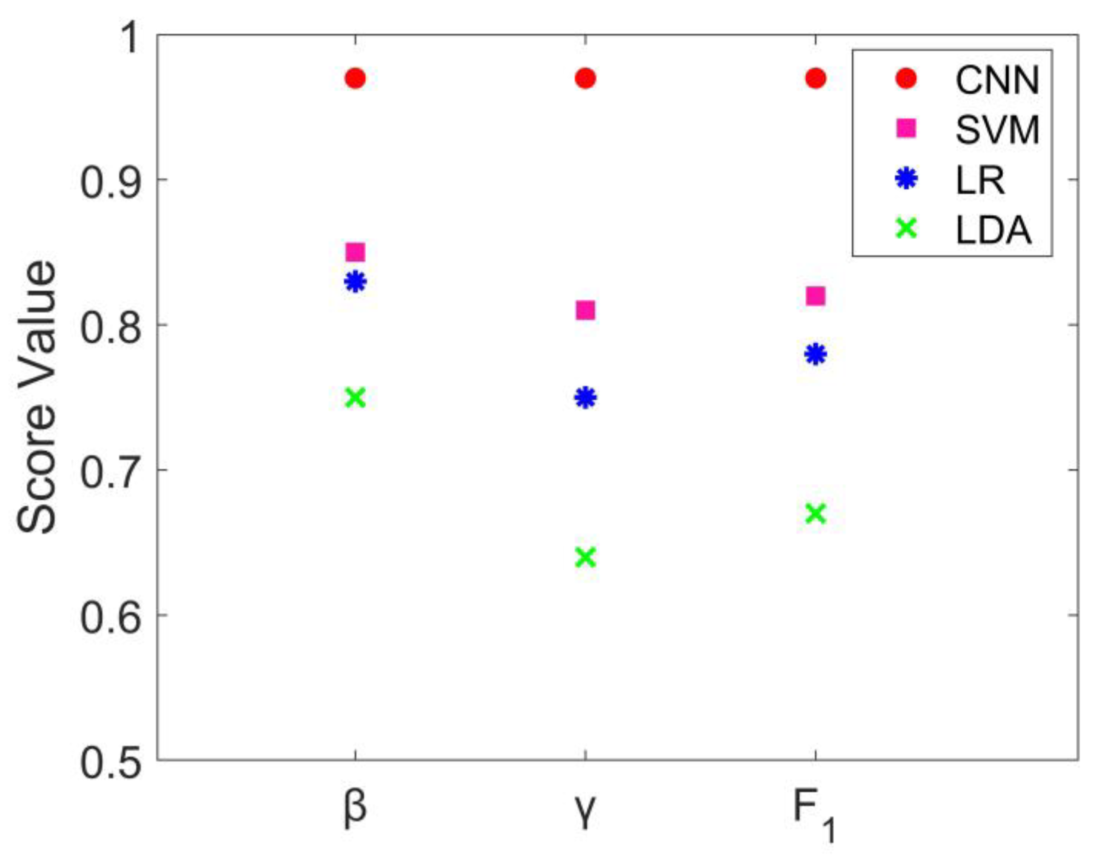
3.1. Classification Results and Performance Comparison

The 660 training spectra and their corresponding labeled rock type values were fed into the CNN, the LR, the SVM, and the LDA model, respectively. During the training phase, the parameters of each model were dynamically adjusted to enable the predicted output to well match the real rock type label. Generally speaking, for almost all machine learning algorithms, the classification correct rate in the training process can reach exactly 100%, and this work is no exception. All four machine learning models could achieve β = γ = F 1 = 1 for each rock type in the training (for the CNN model, this could be achieved as early as in the 4th or 5th step iteration), which was nothing special.
After the training, each of the four models would be fed with the 60 validation set spectra to evaluate whether the model had been well trained. The validation results indicated that each model was well trained since each one could make an absolutely correct rock classification, i.e., β = γ = F 1 = 1 for each rock type. By further calculating the Brier score according to Equation (4) ( N = 720 and M = 12 ), one can find that the Brier scores of the CNN, the LR, and the LDA are all 0.000000, while the Brier score of the SVM is 0.000524. Despite the difference seeming not large, this result has indicated that the four models do not have equal prediction capabilities. The prediction ability discrepancy would be more significant in the results for the testing set, as will be demonstrated in the following.
After the validation, which had verified that each model was mature enough, the 720 completely untrained spectra in the testing set were input into the models to test their genuine generalization capabilities. The classification correct rate of each of the four models is 0.966667 (CNN), 0.851389 (SVM), 0.833333 (LR), and 0.750000 (LDA), respectively. Apparently, the CNN has the highest overall accuracy. The more detailed accuracy information, revealed by β, γ, and F1 scores are listed in Table 4.
A comparison of the average values (averaging upon the 12 samples) of the three scores for the four methods is shown in Figure 9, and the superiority of the CNN is conspicuous. Moreover, although the performance of the other three models seems acceptable regarding the average scores, each of the three models actually contains several low scores, indicating many imprecise prediction cases for certain samples. In fact, the SVM can hardly discriminate the potash feldspar from the kaolinite, while the LDA cannot distinguish the andesite from the montmorillonite, just to name a few.
The high error rates in these predictions are mainly due to the similar chemical compositions of the certain rock samples. As illustrated in Figure 6, the spectra of kaolinite and potash feldspar are similar, and this is also true for andesite and montmorillonite. Although such similarity in the compositions and the spectra has brought great challenges to the three conventional algorithms, the testing results demonstrate that the proposed CNN model can discriminate these samples with high accuracy, achieving a full or nearly full F1 score for all the rock types listed in Table 4.
Figure 10 displays the Brier scores of the four models on the testing set. Unlike the case in the validation, the four Brier scores are clearly different in the testing. Either the LR or the LDA model, which have achieved a zero Brier score in the validation, behave much more poorly in the testing, implying that there exists considerable over-fitting in the training and the model used in this study does not have good generalization capability. The SVM performs the poorest in the validation, but it is the second best model among the four in terms of both overall correct rate and Brier score, indicating that it does not suffer from over-fitting and hence has a relatively great generalization ability. The CNN model obviously achieves a much lower Brier score than the other three models in the testing, thereby demonstrating remarkable superiority in prediction accuracy as well as generalization competence.
Since the CNN is the best performing model, a few more investigations have been carried out about the prediction performance of the CNN. Specifically, the dependence of the CNN performance on the testing set versus the validation set size has been examined. Adding the number of spectra in the validation set can increase the diversity of the validation set. This would be beneficial to model optimization according to the validation results, so that the performance on the testing set can be improved. On the other hand, adding the validation set size naturally means reducing the training set size within the data partition framework in this research. This is definitely unfavorable to the training of machine learning models (especially for deep learning models like CNN), and hence the performance on the testing set would be worsened. Therefore, it is interesting to change the validation set size to inspect the comprehensive impact of the two competitive effects mentioned above.
According to the data partition scheme described in Section 2.5, from each rock sample in Dataset I, five spectra are randomly selected to constitute the validation set. Denote NV as the number of spectra contributed by each sample for validation, then this scheme can be expressed as NV = 5. Besides the normal scheme of NV = 5, several other NV values have been tried, i.e., NV = 8, 10, 12, and 15 (also random spectra selection for each NV value). With the five different NV values, the overall classification correct rate of the CNN on the testing set is 0.966667, 0.912500, 0.897222, 0.888888, and 0.865278, respectively. It can be found that the classification accuracy slowly decays with the enlargement of the validation set size, revealing that the shrinkage of the training set size can really bring a considerable negative effect to the model training. By the way, it is noteworthy that the lowest CNN accuracy in this special investigation (0.865278) is still a bit higher than the second best model in the normal data partition scheme (SVM, 0.851389), indicating the great superiority of the deep learning CNN model.

3.2. Discussion

It is the specific LIBS spectral features that dictate the performance of a chemometric model. Therefore, the more powerful a machine learning method is in feature mining, the better performance it may achieve. The outstanding analytical capability of the CNN model mainly roots in the convolution operations, which thoroughly mine the correlation between the adjacent data points in a LIBS spectrum. However, the other three models, among the many other common machine learning models, may just regard the spectrum as thousands of isolated data points, and hence the inherent unity and internal correlation of the spectrum cannot be fully utilized.
As mentioned in Section 2.2, only a primary preprocessing has been carried out in this study. It is believed that the CNN model can perform well without further preprocessing, such as spectrum smoothing, continuum baseline removal, etc., as verified by the testing results. Such inference is made because only dark background is regarded as pure noise, while other kinds of “noises” (e.g., the continuum baseline) are thought of as inherent parts of the spectrum, which, in fact, may be partially beneficial to the feature extraction of the CNN. The competence to handle simply preprocessed spectra indicates that the CNN can be a highly efficient tool in real-time analysis, which may be a significant advantage in planetary geology researches.
Despite the excellent performance of the CNN, it should be noted that deep learning algorithms such as CNN have disadvantages. One of the most prominent defects is the “black box” nature. The CNN can establish extremely complicated input–output correlations but would reveal little information beyond the input and the output. The features “learned” by the CNN model might be too abstract, and the result interpretation is definitely difficult. Exploring the ways to enhance the interpretability of the deep learning CNN is beyond the scope of this paper, but it would be a great research direction for LIBS chemometrics researchers in the future.
Another disadvantage is relevant to training sample quantity. As demonstrated in the last part of Section 3.1, a large enough training set size is crucial to the CNN model. As a matter of fact, deep learning algorithms like CNN can perform well only when a great number of training samples are available, which is actually impossible in some scenarios in reality. It is noteworthy that only 12 types of rock sample have been employed in this study, which is a relatively small sample set compared to some previous great studies [58]. However, the total number of the LIBS spectra (more than 1400) may guarantee the credibility of the results to some extent. The preliminary tests imply that CNN-supported LIBS classification is a promising methodology for analyzing the MarSCoDe data of Tianwen-1 Mars mission. More experiments with larger sample sets (i.e., including more kinds of target samples) will be carried out in future studies.
Moreover, a newly established large-scale experimental platform able to realize a high-degree simulation of Martian atmospheric environment has been put into use [59]. Thanks to the great volume of this facility, not only the target samples but also the LIBS instrument (e.g., a duplicate laboratory model of MarSCoDe) can be placed in the simulated Martian environment. The long track inside the sample cabin also enables the LIBS detection distance to easily vary from 1.5 m to 7 m, which would be greatly beneficial to the simulation of field detection scenario on Mars and the investigation of the LIBS sampling distance effect.
With more dedicated reference samples and the excellent experimental platform, more LIBS data highly similar to those in real in situ detection will be achieved for further inspection.

4. Conclusions

As one of the six scientific payloads on Zhurong rover for the Tianwen-1 Mars mission, MarSCoDe utilizes LIBS technology to conduct stand-off detection of the chemical compositions of the rocks and soils on Martian surface. This study has proposed a deep CNN model to classify 12 types of rock samples based on the LIBS spectra, which were collected by MarSCoDe in Tianwen-1 pre-flight experiments. The LIBS measurements were partially mimicking the scenario of field operation on Mars, as the rock samples were placed in a simulated Martian atmospheric environment. There are 1440 LIBS spectra in all, which are divided into three datasets, namely a training set, a validation set, and a testing set. The classification task is challenging because the compositions of some different types of rock samples are quite similar, and meanwhile, the compositions of some identical types of rock samples are slightly different. The classification performance of the CNN method has been evaluated by precision score, recall score, F1 score, and Brier score. The results of the testing indicate that the CNN model has prominent superiority in terms of classification accuracy over conventional machine learning methods (LR, SVM, and LDA). The effect of the validation set size upon the CNN competence has also been investigated, probably providing reference for other researchers on data partition strategy.
With remarkable prediction accuracy and high processing efficiency, the CNN model adopted in this work is demonstrated to be a promising rock identification and classification method based on LIBS spectra. The developed CNN-LIBS methodology is expected to be applied to the spectra data from MarSCoDe field detection in the future.

Author Contributions

Conceptualization, F.Y. and L.L.; formal analysis, F.Y. and L.L.; methodology, W.X., F.Y., L.L. and X.L.; writing—original draft, F.Y.; writing—review and editing, Z.C., X.X., L.J., Y.C. and L.L.; supervision, W.X. and R.S. All authors have read and agreed to the published version of the manuscript.

Funding

This work was funded by National Natural Science Foundation of China (NSFC) (No. 11904378) and Natural Science Foundation of Shanghai (No. 22ZR1472400). This work also gained support from China National Space Administration (CNSA) and the National Natural Science Foundation (No. U1931211), Key Laboratory of Lunar and Deep Space Exploration, CAS (No. LDSE201904), and Pre-research Project on Civil Aerospace Technologies (No. D020102).

Data Availability Statement

Not applicable.

Conflicts of Interest

The authors declare no conflict of interest.

References

  1. Rusak, D.A.; Castle, B.C.; Smith, B.W.; Winefordner, J.D. Fundamentals and applications of laser-induced breakdown spectroscopy. Crit. Rev. Anal. Chem. 1997, 27, 257–290. [Google Scholar] [CrossRef]
  2. Harmon, R.S.; Remus, J.; McMillan, N.J.; McManus, C.; Collins, L.; Gottfried, J.L., Jr.; DeLucia, F.C.; Miziolek, A.W. LIBS analysis of geomaterials: Geochemical fingerprinting for the rapid analysis and discrimination of minerals. Appl. Geochem. 2009, 24, 1125–1141. [Google Scholar] [CrossRef]
  3. Gaudiuso, R.; Ewusi-Annan, E.; Melikechi, N.; Sun, X.Z.; Liu, B.Y.; Campesato, L.F.; Merghoub, T. Using LIBS to diagnose melanoma in biomedical fluids deposited on solid substrates: Limits of direct spectral analysis and capability of machine Learning. Spectrochim. Acta Part B At. Spectrosc. 2018, 146, 106–114. [Google Scholar] [CrossRef]
  4. Werheit, P.; Fricke-Begemann, C.; Gesing, M.; Noll, R. Fast single piece identification with a 3D scanning LIBS for aluminium cast and wrought alloys recycling. J. Anal. At. Spectrom. 2011, 26, 2166–2174. [Google Scholar] [CrossRef]
  5. Senesi, G.S.; Dell’Aglio, M.; Gaudiuso, R.; De Giacomo, A.; Zaccone, C.; De Pascale, O.; Miano, T.M.; Capitelli, M. Heavy metal concentrations in soils as determined by laser-induced breakdown spectroscopy (LIBS), with special emphasis on chromium. Environ. Res. 2009, 109, 413–420. [Google Scholar] [CrossRef]
  6. Liu, X.D.; Feng, X.P.; He, Y. Rapid discrimination of the categories of the biomass pellets using laser-induced breakdown spectroscopy. Renew. Energy 2019, 143, 176–182. [Google Scholar] [CrossRef]
  7. Burger, M.; Skrodzki, P.J.; Finney, L.A.; Nees, J.; Jovanovic, I. Remote Detection of Uranium Using Self-Focusing Intense Femtosecond Laser Pulses. Remote Sens. 2020, 12, 1281. [Google Scholar] [CrossRef] [Green Version]
  8. Shi, Q.; Niu, G.H.; Lin, Q.Y.; Xu, T.; Li, F.J.; Duan, Y.X. Quantitative analysis of sedimentary rocks using laser-induced breakdown spectroscopy: Comparison of Support Vector Regression and Partial Least Squares Regression Chemometric Methods. J. Anal. At. Spectrom. 2015, 30, 2384–2393. [Google Scholar] [CrossRef]
  9. Chatterjee, S.; Singh, M.; Biswal, B.P.; Sinha, U.K.; Patbhaje, S.; Sarkar, A. Application of laser-induced breakdown spectroscopy (LIBS) coupled with PCA for rapid classification of soil samples in geothermal areas. Anal. Bioanal. Chem. 2019, 411, 2855–2866. [Google Scholar] [CrossRef]
  10. Wiens, R.C.; Maurice, S.; Barraclough, B.; Saccoccio, M.; Barkley, W.C.; Bell, J.F., III; Bender, S.; Bernardin, J.; Blaney, D.; Blank, J.; et al. The ChemCam Instrument Suite on the Mars Science Laboratory (MSL) Rover: Body Unit and Combined System Tests. Space Sci. Rev. 2012, 170, 167–227. [Google Scholar] [CrossRef]
  11. Wiens, R.C.; Maurice, S.; Lasue, J.; Forni, O.; Anderson, R.B.; Clegg, S.; Bender, S.; Blaney, D.; Barraclough, B.; Cousin, A.; et al. Pre-flight calibration and initial data processing for the ChemCam laser-induced breakdown spectroscopy instrument on the Mars Science Laboratory rover. Spectrochim. Acta Part B At. Spectrosc. 2013, 82, 1–27. [Google Scholar] [CrossRef]
  12. Maurice, S.; Wiens, R.C.; Saccoccio, M.; Barraclough, B.; Gasnault, O.; Forni, O.; Mangold, N.; Baratoux, D.; Bender, S.; Berger, G.; et al. The ChemCam Instrument Suite on the Mars Science Laboratory (MSL) Rover: Science Objectives and Mast Unit Description. Space Sci. Rev. 2012, 170, 95–166. [Google Scholar] [CrossRef]
  13. Sautter, V.; Fabre, C.; Forni, O.; Toplis, M.J.; Cousin, A.; Ollila, A.M.; Meslin, P.Y.; Maurice, S.; Wiens, R.C.; Baratoux, D.; et al. Igneous mineralogy at Bradbury Rise: The first ChemCam campaign at Gale crater. J. Geophys. Res. Planets 2014, 119, 30–46. [Google Scholar] [CrossRef] [Green Version]
  14. Boucher, T.F.; Ozanne, M.V.; Carmosino, M.L.; Dyar, M.D.; Mahadevan, S.; Breves, E.A.; Lepore, K.H.; Clegg, S.M. A study of machine learning regression methods for major elemental analysis of rocks using laser-induced breakdown spectroscopy. Spectrochim. Acta Part B At. Spectrosc. 2015, 107, 1–10. [Google Scholar] [CrossRef]
  15. Schröder, S.; Meslin, P.-Y.; Gasnault, O.; Maurice, S.; Cousin, A.; Wiens, R.C.; Rapin, W.; Dyar, M.; Mangold, N.; Forni, O.; et al. Hydrogen detection with ChemCam at Gale crater. Icarus 2015, 249, 43–61. [Google Scholar] [CrossRef]
  16. Nachon, M.; Mangold, N.; Forni, O.; Kah, L.C.; Cousin, A.; Wiens, R.C.; Anderson, R.; Blaney, D.; Blank, J.; Calef, F.; et al. Chemistry of diagenetic features analyzed by ChemCam at Pahrump Hills, Gale crater, Mars. Icarus 2017, 281, 121–136. [Google Scholar] [CrossRef]
  17. Rivera-Hernández, F.; Sumner, D.Y.; Mangold, N.; Stack, K.M.; Forni, O.; Newsom, H.; Williams, A.; Nachon, M.; L’Haridon, J.; Gasnault, O.; et al. Using ChemCam LIBS data to constrain grain size in rocks on Mars: Proof of concept and application to rocks at Yellowknife Bay and Pahrump Hills, Gale crater. Icarus 2019, 321, 82–98. [Google Scholar] [CrossRef]
  18. Wiens, R.C.; Maurice, S.; McCabe, K.; Cais, P.; Anderson, R.B.; Beyssac, O.; Bonal, L.; Clegg, S.; Deflores, L.; Dromart, G.; et al. The SuperCam Remote Sensing Instrument Suite for Mars 2020. In Proceedings of the 47th Lunar and Planetary Science Conference, The Woodlands, TX, USA, 21–25 March 2016. [Google Scholar]
  19. Manrique, J.A.; Lopez-Reyes, G.; Cousin, A.; Rull, F.; Maurice, S.; Wiens, R.C.; Madsen, M.B.; Madariaga, J.M.; Gasnault, O.; Aramendia, J.; et al. SuperCam Calibration Targets: Design and Development. Space Sci. Rev. 2020, 216, 138. [Google Scholar] [CrossRef]
  20. Maurice, S.; Wiens, R.C.; Bernardi, P.; Caïs, P.; Robinson, S.; Nelson, T.; Gasnault, O.; Reess, J.-M.; Deleuze, M.; Rull, F.; et al. The SuperCam Instrument Suite on the Mars 2020 Rover: Science Objectives and Mast-Unit Description. Space Sci. Rev. 2021, 217, 47. [Google Scholar] [CrossRef]
  21. Wiens, R.C.; Maurice, S.; Robinson, S.H.; Nelson, A.E.; Cais, P.; Bernardi, P.; Newell, R.T.; Clegg, S.; Sharma, S.K.; Storms, S.; et al. The SuperCam Instrument Suite on the NASA Mars 2020 Rover: Body Unit and Combined System Tests. Space Sci. Rev. 2021, 217, 4. [Google Scholar] [CrossRef]
  22. Anderson, R.B.; Forni, O.; Cousin, A.; Wiens, R.C.; Clegg, S.M.; Frydenvang, J.; Gabriel, T.S.; Ollila, A.; Schröder, S.; Beyssac, O.; et al. Post-landing major element quantification using SuperCam laser induced breakdown spectroscopy. Spectrochim. Acta Part B At. Spectrosc. 2022, 188, 106347. [Google Scholar] [CrossRef]
  23. Xu, W.M.; Liu, X.F.; Yan, Z.X.; Li, L.N.; Zhang, Z.Q.; Kuang, Y.W.; Jiang, H.; Yu, H.; Yang, F.; Liu, C.; et al. The MarSCoDe Instrument Suite on the Mars Rover of China’s Tianwen-1 Mission. Space Sci. Rev. 2021, 217, 64. [Google Scholar] [CrossRef]
  24. Cousin, A.; Sautter, V.; Payré, V.; Forni, O.; Mangold, N.; Gasnault, O.; Le Deit, L.; Johnson, J.; Maurice, S.; Salvatore, M.; et al. Classification of igneous rocks analyzed by ChemCam at Gale crater, Mars. Icarus 2017, 288, 265–283. [Google Scholar] [CrossRef]
  25. Yang, G.; Qiao, S.; Chen, P.; Ding, Y.; Tian, D. Rock and soil classification using PLS-DA and SVM combined with a laser-induced breakdown spectroscopy library. Plasma Sci. Technol. 2015, 17, 656–663. [Google Scholar] [CrossRef]
  26. Vítková, G.; Novotný, K.; Prokeš, L.; Hrdlička, A.; Kaiser, J.; Novotný, J.; Malina, R.; Prochazka, D. Fast identification of biominerals by means of stand-off laser-induced breakdown spectroscopy using linear discriminant analysis and artificial neural networks. Spectrochim. Acta Part B At. Spectrosc. 2012, 73, 1–6. [Google Scholar] [CrossRef]
  27. Yelameli, M.; Thornton, B.; Takahashi, T.; Weerkoon, T.; Ishii, K. Classification and statistical analysis of hydrothermal seafloor rocks measured underwater using laser-induced breakdown spectroscopy. J. Chemometr. 2019, 33, e3092. [Google Scholar] [CrossRef]
  28. Bi, Y.; Zhang, Y.; Yan, J.; Wu, Z.; Li, Y. Classification and discrimination of minerals using laser induced breakdown spectroscopy and Raman spectroscopy. Plasma Sci. Technol. 2015, 17, 923–927. [Google Scholar] [CrossRef] [Green Version]
  29. D’Andrea, E.; Pagnotta, S.; Grifoni, E.; Lorenzetti, G.; Legnaioli, S.; Palleschi, V.; Lazzerini, B. An artificial neural network approach to laser-induced breakdown spectroscopy quantitative analysis. Spectrochim. Acta Part B At. Spectrosc. 2014, 99, 52–58. [Google Scholar] [CrossRef]
  30. Campanella, B.; Grifoni, E.; Legnaioli, S.; Lorenzetti, G.; Pagnotta, S.; Sorrentino, F.; Palleschi, V. Classification of wrought aluminum alloys by Artificial Neural Networks evaluation of Laser Induced Breakdown Spectroscopy spectra from aluminum scrap samples. Spectrochim. Acta Part B At. Spectrosc. 2017, 134, 52–57. [Google Scholar] [CrossRef]
  31. Liu, J.C.; Osadchy, M.; Ashton, L.; Foster, M.; Solomone, C.J.; Gibson, S.J. Deep convolutional neural networks for Raman spectrum recognition: A unified solution. Analyst 2017, 142, 4067–4074. [Google Scholar] [CrossRef]
  32. Acquarelli, J.; van Laarhoven, T.; Gerretzen, J.; Tran, T.N.; Buydens, L.M.C.; Marchiori, E. Convolutional neural networks for vibrational spectroscopic data analysis. Anal. Chim. Acta 2017, 954, 22–31. [Google Scholar] [CrossRef] [PubMed] [Green Version]
  33. Lu, C.X.; Wang, B.; Jiang, X.P.; Zhang, J.N.; Niu, K.; Yuan, Y.W. Detection of K in soil using time-resolved laser-induced breakdown spectroscopy based on convolutional neural networks. Plasma Sci. Technol. 2019, 21, 034014. [Google Scholar] [CrossRef]
  34. Krizhevsky, A.; Sutskever, I.; Hinton, G.E. ImageNet Classification with Deep Convolutional Neural Networks. Commun. ACM 2017, 60, 84. [Google Scholar] [CrossRef] [Green Version]
  35. Simonyan, K.; Zisserman, A. Very Deep Convolutional Networks for Large-Scale Image Recognition. arXiv 2015, arXiv:1409.1556. [Google Scholar]
  36. Li, L.N.; Liu, X.F.; Xu, W.M.; Wang, J.Y.; Shu, R. A laser-induced breakdown spectroscopy multi-component quantitative analytical method based on a deep convolutional neural network. Spectrochim. Acta Part B At. Spectrosc. 2020, 169, 105850. [Google Scholar] [CrossRef]
  37. Yang, F.; Li, L.N.; Xu, W.M.; Liu, X.F.; Cui, Z.C.; Jia, L.C.; Liu, Y.; Xu, J.H.; Chen, Y.W.; Xu, X.S.; et al. Laser-induced breakdown spectroscopy combined with a convolutional neural network: A promising methodology for geochemical sample identification in Tianwen-1 Mars mission. Spectrochim. Acta Part B At. Spectrosc. 2022, 192, 106417. [Google Scholar] [CrossRef]
  38. Wan, W.X.; Wang, C.; Li, C.L.; Wei, Y. China’s first mission to Mars. Nat. Astron. 2020, 4, 721. [Google Scholar] [CrossRef]
  39. Weitz, N.; Zanetti, M.; Osinski, G.R.; Fastook, J.L. Modeling concentric crater fill in Utopia Planitia, Mars, with an ice flow line model. Icarus 2018, 308, 209–220. [Google Scholar] [CrossRef]
  40. Head, J.W.; Kreslavsky, M.A.; Pratt, S. Northern lowlands of Mars: Evidence for widespread volcanic flooding and tectonic deformation in the Hesperian period. J. Geophys. Res. 2002, 107, 5003. [Google Scholar] [CrossRef]
  41. Soare, J.; Osinski, G.R.; Roehm, C.L. Thermokarst lakes and ponds on Mars in the very recent (late Amazonian) past. Earth Planet. Sc. Lett. 2008, 272, 382–393. [Google Scholar] [CrossRef]
  42. Lefort, A.; Russell, P.S.; Thomas, N.; McEwen, A.S.; Dundas, C.M.; Kirk, R.L. Observations of periglacial landforms in Utopia Planitia with the High Resolution Imaging Science Experiment (HiRISE). J. Geophys. Res. 2009, 114, E04005. [Google Scholar] [CrossRef]
  43. Morgenstern, A.; Hauber, E.; Reiss, D.; Gasselt, S.V.; Grosse, G.; Schirrmeister, L. Deposition and degradation of a volatile-rich layer in Utopia Planitia, and implications for climate history on Mars. J. Geophys. Res. 2007, 112, E06010. [Google Scholar] [CrossRef] [Green Version]
  44. Ulrich, M.; Morgenstern, A.; Günther, F.; Reiss, D.; Bauch, K.E.; Hauber, E.; Rössler, S.; Schirrmeister, L. Thermokarst in Siberian ice-rich permafrost: Comparison to asymmetric scalloped depressions on Mars. J. Geophys. Res. 2010, 115, E10009. [Google Scholar] [CrossRef] [Green Version]
  45. Clark, B.C.; Baird, A.K.; Rose, H.J.; Priestley, T.; Keil, K.; Castro, A.J.; Kelliher, W.C.; Rowe, C.D.; Evans, P.H. Inorganic analyses of Martian surface samples at the Viking landing sites. Science 1976, 194, 1283–1288. [Google Scholar] [CrossRef] [PubMed]
  46. Bandfield, J.L.; Hamilton, V.E.; Christensen, P.R. A global view of Martian surface compositions from MGS-TES. Science 2000, 287, 1626–1630. [Google Scholar] [CrossRef] [Green Version]
  47. Brennetot, R.; Lacour, J.L.; Vors, E.; Rivoallan, A.; Vailhen, D.; Maurice, S. Mars Analysis by Laser-Induced Breakdown Spectroscopy (MALIS): Influence of Mars Atmosphere on Plasma Emission and Study of Factors Influencing Plasma Emission with the use of Doehlert Designs. Appl. Spectrosc. 2003, 57, 744–752. [Google Scholar] [CrossRef]
  48. Liu, C.; Ling, Z.; Zhang, J.; Wu, Z.; Bai, H.; Liu, Y. A Stand-Off Laser-Induced Breakdown Spectroscopy (LIBS) System Applicable for Martian Rocks Studies. Remote Sens. 2021, 13, 4773. [Google Scholar] [CrossRef]
  49. Maas, A.L.; Hannun, A.Y.; Ng, A.Y. Rectifier nonlinearities improve neural network acoustic models. Proc. ICML 2013, 30, 3. [Google Scholar]
  50. Bishop, C.M. Pattern Recognition and Machine Learning; Springer: New York, NY, USA, 2006. [Google Scholar]
  51. Hinton, G.E.; Srivastava, N.; Krizhevsky, A.; Sutskever, I.; Salakhutdinov, R.R. Improving neural networks by preventing co-adaptation of feature detectors. arXiv 2012, arXiv:1207.0580. [Google Scholar]
  52. Hastie, T.; Tibshirani, R.; Friedman, J. The Elements of Statistical Learning: Data Mining, Inference, and Prediction; Springer: New York, NY, USA, 2009. [Google Scholar]
  53. Peng, C.J.; Lee, K.L.; Ingersoll, G.M. An Introduction to Logistic Regression Analysis and Reporting. J. Educ. Res. 2002, 96, 3–14. [Google Scholar] [CrossRef]
  54. Tharwat, A.; Gaber, T.; Ibrahim, A.; Hassanien, A.E. Linear discriminant analysis: A detailed tutorial. AI Commun. 2017, 30, 169–190. [Google Scholar] [CrossRef] [Green Version]
  55. Pedregosa, F.; Varoquaux, G.; Gramfort, A.; Michel, V.; Thirion, B.; Grisel, O.; Blondel, M.; Prettenhofer, P.; Weiss, R.; Dubourg, V.; et al. Scikit-learn: Machine Learning in Python. J. Mach. Learn. Res. 2011, 12, 2825–2830. [Google Scholar]
  56. Powers, D.M.W. Evaluation: From precision, recall and F-measure to ROC, informedness, markedness and correlation. J. Mach. Learn. Technol. 2011, 2, 37–63. [Google Scholar]
  57. Gerds, T.A.; Cai, T.; Schumacher, M. The performance of risk prediction models. Biom. J. 2008, 50, 457–479. [Google Scholar] [CrossRef] [PubMed]
  58. Clegg, S.M.; Wiens, R.C.; Anderson, R.; Forni, O.; Frydenvang, J.; Lasue, J.; Cousin, A.; Payré, V.; Boucher, T.; Dyar, M.D.; et al. Recalibration of the Mars Science Laboratory ChemCam instrument with an expanded geochemical database. Spectrochim. Acta Part B At. Spectrosc. 2017, 129, 64–85. [Google Scholar] [CrossRef]
  59. Cui, Z.; Jia, L.; Li, L.; Liu, X.; Xu, W.; Shu, R.; Xu, X. A Laser-Induced Breakdown Spectroscopy Experiment Platform for High-Degree Simulation of MarSCoDe In Situ Detection on Mars. Remote Sens. 2022, 14, 1954. [Google Scholar] [CrossRef]
Figure 1. A MOLA map of Mars with the landing site of Tianwen-1 lander marked out by the red pentagram (near the site of Viking 2). The base map is MOLA DEM37, available at https://astrogeology.usgs.gov/search/map/Mars/GlobalSurveyor/MOLA/Mars_MGS_MOLA_DEM_mosaic_global_463m, accessed on 21 August 2022).
Remotesensing 14 05343 g001
Figure 2. Diagram of Tianwen-1 lander (right) and Zhurong rover (left), which is equipped with the MarSCoDe instrument. The original picture is available on the Internet.
Remotesensing 14 05343 g002
Figure 3. Diagram of the LIBS experimental setup, including the MarSCoDe instrument and the Martian atmosphere simulation chamber holding the rock samples. The vacuum chamber was filled with CO2 gas, with a pressure of 933 Pa. The laser-target distance was kept 3.0 m.
Remotesensing 14 05343 g003
Figure 4. Demonstration of some sample pellets: (a) andesite, (b) dolomite, (c) kaolinite, (d) basalt. Some vaguely visible black dots are laser ablation craters.
Remotesensing 14 05343 g004
Figure 5. Typical preprocessed LIBS spectra of the twelve types of rock samples. DN stands for digital number.
Remotesensing 14 05343 g005
Figure 6. LIBS spectra of certain rock samples with similar chemical compositions, with some characteristic emission lines indicated. (a) The potash feldspar, (b) the andesite, (c) the kaolinite, (d) the montmorillonite. DN stands for digital number.
Remotesensing 14 05343 g006
Figure 7. The LIBS spectrum of the potash feldspar sample in the training set (reference material, red dashed line) and that in the testing set (natural sample, blue line). Each spectrum is an average of the 60 spectra. DN stands for digital number.
Remotesensing 14 05343 g007
Figure 8. (a) Schematic topology and relevant parameters of the designed CNN. (b) Demonstration of data operation by the convolutional layer and the max-pooling layer, and explanation of the main functions of the two kinds of layers.
Remotesensing 14 05343 g008
Figure 9. Comparison of the average precision score (β), recall score (γ), and F1 score values for the four methods. The three kinds of scores for each of the 12 samples can be calculated based on Equations (1)–(3), and for each kind of score the average score displayed herein is the mean of the 12 scores corresponding to the 12 samples. The red circles stand for the result of the CNN, magenta squares for the LR, blue stars for the SVM, and green crosses for the LDA.
Remotesensing 14 05343 g009
Figure 10. Comparison of Brier scores of the four methods on the testing set.
Remotesensing 14 05343 g010
Table 1. Main technical specifications of the MarSCoDe.
ParameterValue
Laser pulse width4 ns
Laser pulse energy9 mJ
Laser wavelength1064 nm
Laser repetition rate1 Hz, 2 Hz, 3 Hz
Overall spectral range240–850 nm
Number of spectral channels3
Pixels per spectral channel1800
Detection distance1.6–7 m
Table 2. The main components of the twelve types of rocks. The concentration value is expressed by weight percentage (in unit of %). The cross symbol denotes the case that the certain component is not included in the sample.
No.Rock TypeSiO2Al2O3Fe2O3CaOMgOK2ONa2O
1Andesite60.6216.174.95.21.721.893.86
2Dolomite0.0210.0170.22432.1120.370.00110.023
3Opal68.98××××××
4Kaolinite43.4134.771.50.0380.0690.780.045
5Potash feldspar66.2618.630.190.760.0549.63.69
6Montmorillonite77.8913.78×2.811.4×0.28
7Diopside53.401.380.4324.4018.310.150.26
8Basalt44.6413.8313.48.817.772.323.38
9Hematite9.820.4861.730.110.0550.0560.0056
10Olivine40.73×8.670.0450.05××
11Albite67.9619.620.10.480.0150.09811.26
12Gypsum7.211.920.6328.54.920.380.021
Table 3. Description of the LIBS spectra dataset partition.
DatasetDataset ⅠDataset Ⅱ
Training SetValidation SetTesting Set
Spectrum quantity66060720
Table 4. The classification performance of the four methods for the test dataset, evaluated by β, γ, and F1 scores.
Rock TypeCNNLRSVMLDA
βγF1βγF1βγF1βγF1
10.7810.880.330.740.46000000
210.950.98111111000
30.9010.95111111111
411110.50.6710.50.67111
50.970.980.97000000000
610.920.9610.920.9610.510.6710.370.54
70.950.900.9311110.970.98111
810.980.990.880.60.7211110.980.99
9111111111111
10111111111111
1110.880.9411111110.780.88
1211111111110.50.67
Publisher’s Note: MDPI stays neutral with regard to jurisdictional claims in published maps and institutional affiliations.

