Article

PU-WGCN: Point Cloud Upsampling Using Weighted Graph Convolutional Networks

1
School of Science, Beijing University of Civil Engineering and Architecture, Beijing 100044, China
2
Aerospace Information Research Institute, Chinese Academy of Sciences, Beijing 100094, China
*
Author to whom correspondence should be addressed.
Remote Sens. 2022, 14(21), 5356; https://doi.org/10.3390/rs14215356
Submission received: 6 August 2022 / Revised: 15 October 2022 / Accepted: 23 October 2022 / Published: 26 October 2022

Abstract

:
Point clouds are sparse and unevenly distributed, which makes upsampling a challenging task. The current upsampling algorithm encounters the problem that neighboring nodes are similar in terms of specific features, which tends to produce hole overfilling and boundary blurring. The local feature variability of the point cloud is small, and the aggregated neighborhood feature operation treats all neighboring nodes equally. These two reasons make the local node features too similar. We designed the graph feature enhancement module to reduce the similarity between different nodes as a solution to the problem. In addition, we calculate the feature similarity between neighboring nodes based on both spatial information and features of the point cloud, which is used as the boundary weight of the point cloud graph to solve the problem of boundary blurring. We fuse the graph feature enhancement module with the boundary information weighting module to form the weighted graph convolutional networks (WGCN). Finally, we combine the WGCN module with the upsampling module to form a point cloud upsampling network named PU-WGCN. Compared with other upsampling networks, the experimental results show that PU-WGCN can solve the problems of hole overfilling and boundary blurring and improve the upsampling accuracy.

1. Introduction

With the rapid development of 3D scanning technology, the point cloud data of objects in real scenes can be acquired efficiently. The acquired point cloud data are widely used in various fields such as architectural surveys and autonomous vehicles. However, due to the external environment and hardware constraints, laser scanners often produce noisy, non-uniform, and sparse point clouds, which will show obvious limitations. Therefore, upsampling input point cloud processing becomes an indispensable step. The upsampling operation preserves the object geometry, and further completes the missing point cloud, which can improve the point cloud quality and make the point cloud more complete.
The upsampling task of point clouds can increase the number of points efficiently and preserve the important geometric properties of the input point clouds. Moreover, the network requires a uniform distribution of upsampling points. The current study can achieve the reconstruction of point cloud surfaces by meshing, voxel [1], moving least squares smoothing [2], and Poisson surface reconstruction [3]. With the rapid development of deep learning, several scholars have started to use deep learning to classify [4,5], segment [6,7,8,9], upsample [5,10,11,12,13,14,15], and perform other operations on point clouds. Deep learning methods can perform the upsampling of point clouds more efficiently than traditional methods. In the point-based upsampling method, PointNet++ [5] increases the number of points by interpolation. Due to the sparse and nonuniform distribution of the original input point cloud, the interpolation method is not conducive to determining the location of the interpolation points, and instead the upsampling points will produce bias. PU-Net [10] is used to generate new points by duplicating and reshaping features in the feature space. However, the duplication method does not provide information about the location variation of the points, in which case the upsampled points may overlap or be near to the original points. To address the overlapping problem generated by PU-Net, MPU [11] randomly assigns a one-dimensional code with values of −1 and 1 in the upsampling module so that the upsampled points have different position variations. Although this method uses a differentiation strategy, the strategy does not consider geometric information. Because point clouds are irregular and disorderly, the above point-based methods do not work well for upsampling.
In addition to the point-based upsampling method, scholars nowadays also choose to two-dimensionalize and upsample the point cloud. In the upsampling module, PU-GAN [12] regularizes the point cloud by using the grid mechanism first in folding net, and then adds a two-dimensional vector after the replicated feature. It makes the replicated point features have subtle differences. We regularize the point cloud with a grid, but this does not mean that the transformed points are uniformly distributed on the three-dimensional surface. When the surface of the object is complex, the above method will produce an over-smoothing problem. PU-GeoNet [13] performs upsampling work on parametrized two-dimensional surfaces. It maps the upsampled points back to the three-dimensional surface with normal vectors. However, the current upsampling is performed in two dimensions with a loss of geometric information. In addition, the method generates outlier points at the corners of the object. As a result, the planarized point cloud causes the loss of its important information, which leads to ineffective upsampling. Feng et al. [14] proposed neural points to upsample the point cloud with an arbitrary number of points. The point cloud upsampling method based on neural fields [14] can effectively express its geometric information.
With the wide application of convolutional neural networks (CNN), more and more scholars gradually apply the convolutional idea to 3D. The basic idea of point cloud convolution [16,17,18] is to reweight and rearrange the associated features by transforming the matrix. The number of points is huge, so the memory consumption of the transformation matrix is extremely large, which also increases the computation overhead. To solve this problem, DGCNN [19] designed the EdgeConv module by using the idea of graph theory [20]. This module keeps the alignment invariance of the point cloud, and takes better account of the local geometric features of the point cloud. PU-GCN [15] uses the graph convolutional network (GCN) layers to construct point cloud graphs. In GCN networks, points convey information [21] through graph structure and node features. Compared with the duplicated upsampling method, GCN utilizes more local neighborhood information. In PU-GCN, the central node and boundary information are passed as local information of the point cloud. The local neighborhood variability is small and the aggregated neighborhood features operation treats all neighboring nodes equally. The above reasons make the neighboring nodes similar in specific attributes [22,23]. As a result, the upsampling operation of the point cloud can produce oversmoothing problems [21,24]. The oversmoothing problem tends to produce holes being overfilled. In addition, the NodeShuffle [15] mechanism in PU-GCN has no strict restriction on the boundary point cloud. Moreover, this network uses a uniform pattern to constrain the upsampled points in the point cloud graph. As a result, the upsampling points at the object boundaries produce more outliers, which leads to boundary blurring. Outlier points are generated after one round of upsampling learning at the object boundaries, which can be regarded as noise points. Because the learning mode of the upsampling network is multi-round, the boundaries of the objects will be more blurred after multiple upsampling operations.
To solve the problems of hole overfilling and boundary blurring generated by the upsampling network, we propose the graph feature enhancement module and the boundary information weighting module. These two modules are combined with the upsampling module to form an upsampling network called PU-WGCN. Among them, the graph feature enhancement module aims to reduce the similarity between different nodes and enhance the representation of node feature information. In addition, the nodes of the graph network can be selected in GNN by calculating the similarity between nodes. This idea has been applied to various fields to form graph network structures, such as complex network communities, knowledge graphs, recommender systems [25], and drug relationship networks [26]. We apply the idea to the construction of point cloud graphs. The point cloud graph is weighted [27] by calculating the feature similarity [28]. However, it lacks spatial geometry information if we only calculate the similarity for features. Therefore, we calculate the similarity based on both spatial information [29] and features [30] of the point cloud, and use it to weight the boundary information.
Experiments show that the above strategies can solve the problems of hole overfilling and boundary blurring generated by upsampling on point clouds. For the upsampling task, our method can achieve advanced results. In summary, our main contributions are as follows.
  • Neighboring nodes with less variability and the aggregated neighborhood features operation treats all neighboring nodes equally. These two reasons lead to features of neighboring nodes that are too similar. When upsampling at the hole of the object, the network imposes uniform constraints on the upsampling points. As a result, the upsampling network creates the problem of holes being overfilled when increasing the number of points in this local neighborhood. Therefore, we enhance the graph feature information for the purpose of reducing the feature similarity of the point cloud.
  • The current upsampling network has no strict constraints on the boundary points. Moreover, the upsampling network uses uniform pattern to constrain the upsampling points in the point cloud graph. As a result, the boundary point cloud of the object generates outliers, which lead to boundary blurring. To solve this problem, we propose the boundary information weighting module. It weights the boundary information by calculating the point similarity. It makes the upsampling network more boundary-focused.
  • The above two modules are combined with the upsampling module to form the upsampling network named PU-WGCN. PU-WGCN can solve the problems of hole overfilling and boundary blurring generated by upsampling.

2. Relation Work

In this section, we give a brief description of the work related to graph neural networks and GCN-based point cloud processing.

2.1. Graph Convolutional Networks (GCNs)

In real life, a lot of data exists in the form of graphs. For example, social networks, communication networks, etc. The nodes in a graph represent the individuals in the network, and the connected edges represent the connection relationships between the individuals. Kipf et al. [31] extended the convolvable range from Euclidean space to non-Euclidean space when GCN appeared in 2017. Currently, using graph neural networks to process non-Euclidean data is becoming increasingly popular. The selection of nodes and the construction of graphs are important when we use GCN for feature extraction. Otherwise, the network will suffer from oversmoothing problems. Chen et al. [32] found that the topology of the graph has a great impact on the smoothness and the performance of the model. They optimized the topology of the graph by removing interclass edges and adding intraclass edges. Kong et al. [33] improved the GCN performance by graph data augmentation method. This network uses weighted perturbations in the feature space during training to enrich the training data. Asiri et al. [34] proposed the GraphSNN model. This model considers the neighboring subgraph structure, but the structure of the subgraph is fixed. In the case of unknown graph structure, there are some limitations in fixing the graph structure.

2.2. Point Cloud Processing Based on Graph Neural Network

GNNs have emerged as a widespread graph analysis method due to the powerful expressive power of graph structures. GNNs have become popular in methods for 3D point cloud target detection and segmentation. PointGNN [35] uses graph neural networks to predict the class and shape of point clouds. We use the graph structure to preserve the irregularity of the point cloud. The point cloud features are further extracted by updating iterative graph features.

3. Materials and Methods

In this paper, an upsampling network named PU-WGCN is proposed to address the problems of hole overfilling and boundary blurring generated by the upsampling algorithm. The WGCN contains two parts, one is to enhance the graph features, and the other is to weight the boundary information in the point cloud graph. The two parts are described in detail below.

3.1. Weighted Graph Convolutional Networks (WGCN)

3.1.1. Graph Feature Enhancement Module

The local neighborhood is constructed by finding the k neighbor nodes of the central node through the K-nearest neighbor (KNN) algorithm. A point in the point cloud is chosen as the central node arbitrarily and k neighbor nodes are found by the KNN algorithm. We construct the local neighborhood by combining the central node with the neighborhood nodes. Within the local neighborhood, the neighborhood nodes’ information and the central node information are updated by passing through the aggregation operation. The spatial locations of the neighborhood points selected by KNN algorithm are close to each other, so the feature similarity of the neighborhood points is high after feature extraction. Moreover, the aggregated neighborhood feature operation treats all neighboring nodes equally. In addition, the selection of neighborhood points is obtained only by relying on the constraint of Euclidean distance, so the neighborhood nodes may be adjacent to the central node indirectly. When the network upsamples at object holes, the neighboring points may be separated from the center point by the holes. Within this local point cloud graph, when upsampling neighboring points with similar features, the network assumes that the neighboring points are uniformly distributed, and thus the upsampling network can cause the holes to be overfilled. As shown in the right panel of Figure 1, the location of the hole in the chair will be covered, where the red point cloud is the input point cloud and the green point cloud is the point cloud after upsampling. Therefore, strategies are needed to make the neighborhood point features more differentiated. We increase the representation of neighborhood point features by enhancing the graph feature module.
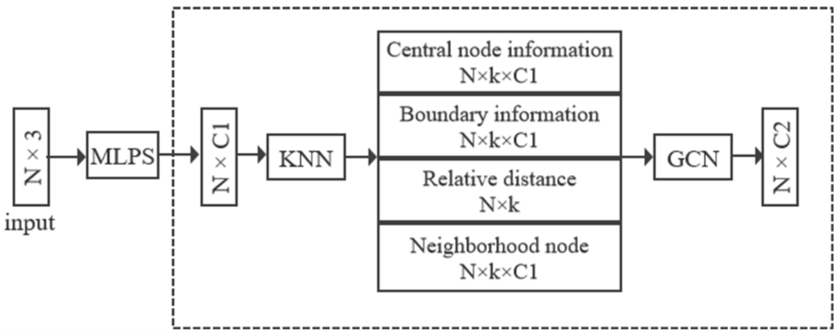
The previous upsampling studies focus on the features of the points and ignore the boundary information of the point cloud. The emergence of the GCN solves this problem. The GCN is utilized as the extracted feature module, as shown in Figure 2. This module is a feature extraction of the input point cloud with the help of central node information and boundary information. In the point cloud graph, we first extract the semantic information of the point cloud by the multilayer perceptron (MLP) operation. Furthermore, the neighborhood nodes are obtained by the KNN algorithm. We calculate the boundary features between the neighborhood nodes and the central node. We also concatenate the node information with the boundary information as the local point cloud graph features. Finally, the feature aggregation operation is performed by GCN to update the features of the points.
In the local point cloud graph, the points are close to each other. Therefore, the spatial location coordinates of individual points differ little. When we apply the MLP to learn the coordinate information, the semantic features obtained are too similar. We substitute them into the GCN module to get similar graph features. The similar graph features enter the upsampling module, and the network scatters the points uniformly in that local neighborhood. In particular, when upsampling at the holes of the object, the network will overfill the holes. What we want to do is to increase the feature representation of the point cloud, so that the upsampling network recognizes the features of each point.
After constructing the point cloud graph, the graph feature enhancement module increases the feature variability of different nodes by enhancing the node information. When upsampling local neighborhoods with hole details, the module enhances the information of the nodes, and the later upsampling network identifies the variability among the nodes. Thereby this module solves the problem of holes being overfilled. As shown in Figure 3, it enhances the features of nodes that are adjacent to each other indirectly. When upsampling is performed, it pulls apart the point cloud covering the object’s hole. The chair shown in Figure 3 retains the geometry of the holes.
The graphical feature enhancement module is used to enhance the point cloud features, the structure of which is shown in Figure 4. Compared with the GCN, it adds neighborhood nodes information and distance information to the construction of the point cloud graph. The purpose of the graph feature enhancement module is to enhance the graph feature information of neighboring nodes and reduce the similarity between different nodes. We use this module to solve the problem of overfilled holes generated by the upsampling network.
The graph feature enhancement module concatenates the central node information, neighborhood nodes information, boundary information, and distance information as local graph information. The upsampling network passes the enhanced information at each point in the local graph, and this operation will help the feature extraction module to obtain more distinguishable node features. The following is the calculation process.
Step 1: Get the neighbor nodes information. The local neighborhood graph is constructed by the KNN algorithm. We obtain the information of each node from the neighborhood graph.
Step 2: Get the central node information. The central node is the central point in the local neighborhood graph. In order to facilitate subsequent calculations, we need to expand the dimension of the central node.
Step 3: Get relative distance information. Because the number of point clouds is huge, the network is computationally overloaded. Therefore, the input points need to be grouped before constructing the point cloud graph. We give a point cloud in a patch as an input to the upsampling network. The input point cloud can be denoted as A = A 1 , A 2 A n R F , where n represents the number of points and F represents the number of feature dimensions. We choose one of the points A i as the center point of the point cloud graph and calculate the distance between this point and the other points in the patch:
D A i , A j = F = 1 C A i F A j F 2 .
Step 4: Get boundary information. We sort the calculated distances and select the k closest points to the centroid as local neighborhood points. Define e i j as the edge feature of the neighborhood point A j pointing to the center point A i and p i j as the point feature. F denotes the feature extraction function. In this paper the feature extraction function is the convolution function. The “⊕” operation refers to the concatenated operation of the point feature:
e i j = F A j A i
p i j = F A i F A j .
Finally, we connect the information obtained from the above calculations as point cloud graph information. We pass the information in the point cloud graph, and the process is represented in the following equation,
f i j = m a x R e l u F A j A i , D + p i j
where A j A i represents the boundary information of the neighboring points, D represents the relative distance information between the neighboring points and the center point, A i represents the center point feature, and A j represents the neighboring point feature. Here, p i j represents the point features. From the above steps we obtain the neighbor nodes information, central node information, relative distance information, and boundary information, respectively. We perform the concatenated operation on these four kinds of information and use them as point cloud graph information. The network aggregates local neighborhood features based on the point cloud graph structure. After that, the Relu activation operation is performed on the local neighborhood features to make the network learn the upsampling task better. Finally, to reduce the computation and video memory, we use the max function to extract its main features. The upsampling network conveys information and updates point features through the above ideas.

3.1.2. Boundary Information Weighting Module

In the point cloud graph, the neighborhood nodes information and the central node information are updated by passing through the aggregation operation. The NodeShuffle mechanism in the PU-GCN upsampling network has no strict restrictions on the boundary points. Furthermore, the upsampled points are uniformly distributed on the network constraints. As a result, the boundary point cloud produces spillover after upsampling. Figure 5 shows the upsampling of the chair, where the red point cloud is the input point cloud and the green point cloud is the point cloud after upsampling. From the figure, it can be seen that the boundary of the chair produces point cloud spillover, and the outliers lead to boundary blurring. Based on this, we weight the boundary information in the point cloud graph. The weighting operation increases the attention of the boundary information, so that the upsampling network can better preserve the boundary of the object.
As shown in Figure 6, we use the red points as the original points of the point cloud graph and the green points as the upsampling points. As can be seen from Figure 6, we mark the back boundary of the chair with a black line, and we can see multiple green points beyond the boundary of the chair. Within the local point cloud graph, we calculate the feature similarity between the original points and the upsampled points separately. The lower similarity indicates that the two points are more different. We regard the upsampled points with low similarity as the points overflowing the boundary. Then, the upsampling network should reduce the attention of the overflow boundary points. Based on this, we use the feature similarity to weight the boundary information. The weighted boundary information acts on the upsampling network. The lower similarity the points have, the less impact the upsampling learning of the network gets. As can be seen from Figure 7, The network then avoids creating new points around the points that overflow the boundary, which solves the problem of boundary blurring.
After constructing the local point cloud graph, we determine the attention of the boundary by calculating the feature similarity of the connected points. For the upsampled points beyond the object boundaries, we reduce their attention by the boundary information weighting operation, which also reduces the information transfer of spillover outliers. In other words, we pull back the outliers that overflow the boundaries, and the operation makes the network retain the boundary information of the objects.
The structure of our proposed boundary information weighting module is shown in Figure 8. In contrast to GCN, this module performs a weighting operation on the boundary information by calculating the feature similarity of the point cloud. We concatenate the central node features with the weighted boundary information as point cloud graph features, which are then substituted into the upsampling network for learning. The module will reduce the focus on neighborhood points with smaller feature similarity. This module will solve the problem of boundary blurring generated by the upsampling network.
The similarity of points can be obtained by computing feature vectors through dynamic update operations of complex networks [27,30], but this method is also computationally complex, and the process is not transparent. Moreover, the method of measuring similarity by calculating the feature distance [29] is more classical. The smaller the calculated distance is, the higher the similarity is. Compared with Manhattan distance and Chebyshev distance, the computation of cosine similarity is relatively small, so cosine similarity is more suitable as a weight. In addition, point cloud features are usually represented as vectors, and the value of Chebyshev equidistance is affected by the dimensionality, whereas cosine similarity is not. To avoid the problem of large distances due to the length of the features, we finally choose the cosine similarity to measure the similarity of the points.
We select a point A i F = C in the point cloud as the center point and a neighborhood point A j F = C in the local neighborhood arbitrarily. F is a joint name to denote the feature dimension, and C denotes the number of feature dimensions of the point cloud after the convolution operation. The ”⊕” operation in Equations (5) and (6) is a concatenated operation that takes the feature information, spatial coordinate information, and distance information of the point cloud. In addition, we connect the position space and distance information of the two points and the network uses the connected features to calculate the cosine similarity:
A i F = C = A i F = C A i F = 3 D
A j F = C = A j F = C A j F = 3 D .
Calculate the cosine similarity as follows:
s = F = 1 C A i × A j F = 1 C A i 2 × F = 1 C A j 2 .
The weighted messaging is as follows,
f i j = m a x R e l u s · e i j + F A i ,
where e i j represents the edge information of neighborhood points, s denotes feature similarity, and A i represents point features. s · e i j is the weighted boundary information. F is the convolution function to extract point features. We concatenate the boundary features with the central node features, and then apply the max and Relu functions to learn the point cloud graph features.
Compared with the original GCN, the boundary information weighting module performs feature weighting on the boundary information. This operation will help the upsampling network to pay more attention to the boundary and retain the boundary.

3.2. PU-WGCN Architecture

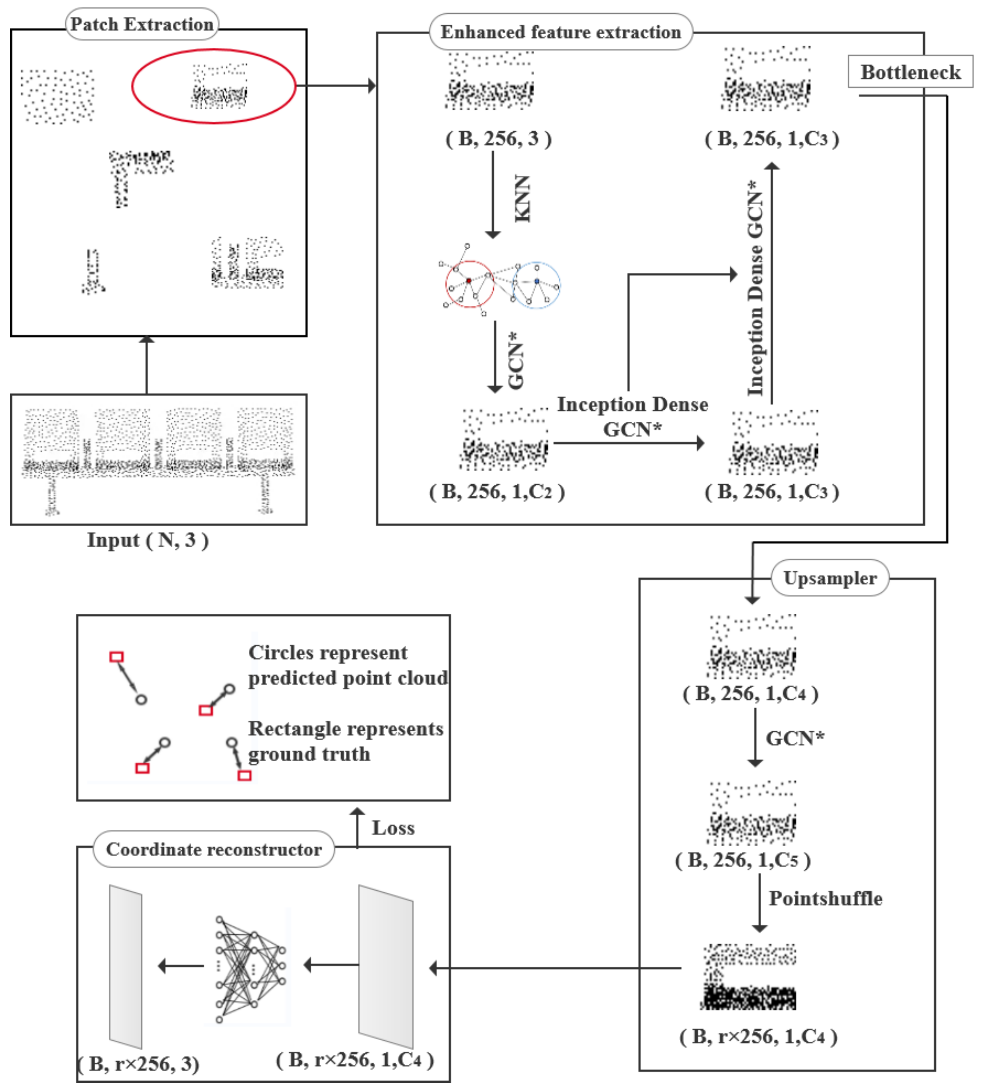
We fuse the above two parts to form the WGCN feature extraction module, and combine the WGCN module with the upsampling module to form the final upsampling network named PU-WGCN. The network framework is shown in Figure 9.
Patch Extraction. We select a series of 3D point cloud models as the input to the network with a size of N × 3 . These 3D models cover almost all aspects of life with various shapes. Among them are point clouds of chairs, motorcycles, cabinets, airplanes, and many other categories. We perform the upsampling operation of point clouds by learning the local point cloud features. The large amount of data in the point clouds makes us take a patch-based approach to upsample the point clouds.
In detail, we crop 50 patchs from each 3D model as the input to the network. We generate the ground truth point clouds in the original mesh by using Poisson disk sampling. The number of input point clouds in each patch is 256, and the ground truth point cloud is 1024.
Enhanced feature extraction. We use the cropped small patch point cloud as the input of the enhanced feature extraction module. First, the point cloud graph is constructed by the KNN algorithm. The information in the point cloud graph contains central nodes, neighboring nodes, relative distance, and weighted boundary information. The constructed point cloud graph is substituted into the GCN* for feature learning. The lower layers in the network are usually used to extract small-scale local features. We use two layers of Inception DenseGCN* for feature learning in the paper in order to enhance the upsampling quality. Then we aggregate the features from different layers. Through this module, we obtain the extracted feature size as N × C 3 . In this paper, we use WGCN as a point cloud graph feature extraction module. Its network structure is shown in Figure 10.
Upsampler. The NodeShuffle module was proposed by Qian et al. [15] originally. It is a graph convolution upsampling module. First, the computation is reduced by a bottleneck layer, the output size of which is N × C 4 . Secondly, we use the WGCN instead of the GCN module. This is done to make the upsampling network more focused on object boundaries and holes. Finally, we upsample the input point cloud of size N × C 4 to a point of size r N × C 4 .
Coordinate reconstructor. We reconstruct the points in the feature space into the coordinate space. The coordinate reconstruction method adopted in the paper is the same as that in PU-GCN [15], which uses two layers of MLPs for this module.
Figure 9 shows the upsampling network graph of a single patch. We use the WGCN module as the feature extraction module GCN* in the upsampling network. The number of input points is N. The number of points in each patch is 256 after the grouping operation. The point cloud in a single patch is increased from 256 to r 256 , where r is the upsampling rate. C 2 , C 3 , C 4 , and C 5 are the number of features of the point cloud after extraction by the feature extraction module.
In the point cloud graph, we have the cosine similarity on the boundary and also introduce the distance and neighborhood point information into the graph structure, which form the WGCN module. The process of information transfer in the point cloud graph is represented as follows:
f i j = m a x R e l u s · e i j + s · F D + F A i + F A j .
Equation (9) can be seen as a combination of Equations (4) and (8). The WGCN feature extraction module is combined with the upsampling module to form the upsampling network named PU-WGCN.

4. Experiments and Results

In this paper, the pu1k dataset is selected to train and test the network performance, and we compare and analyze the experimental results from both quantitative and qualitative perspectives. To verify the effectiveness of the proposed module, we also performed ablation experiments.

4.1. Results and Comparisons

The pu1k dataset [15] is a combination of the PU-GAN dataset [12] and the ShapeNetCore dataset. Compared with the existing upsampled datasets, the pu1k dataset has a richer variety of point clouds and the largest number of point cloud models. There are 1147 point cloud models in this dataset, of which 1020 models are used to train the network and 127 models are used to test the network performance. Therefore, we choose the pu1k dataset for the comparative analysis of experimental results.
All experiments in the paper were conducted on an NVIDIA Tesla V100. The experimental environment built in this paper is CUDA10.1, CUDNN7.6 and GCC7.3. To ensure the objectivity of the experiment, we chose the parameters consistently in each network. We obtain 51,000 patches in the pu1k dataset for network training and 6350 patches for testing. We train 100 epochs on the upsampled network. For a quantitative comparison with previous upsampling networks, we choose Chamfer distance (CD), Hausdroff distance (HD) and point to surface (P2F) as the measure of upsampling network accuracy.
The CD is the distance between the upsampled point cloud and the ground truth point cloud. If this distance is larger, it means that the difference between the two sets of point clouds is greater, and the smaller the distance, the better the upsampling effect. HD describes the degree of similarity between the two sets of point clouds, and measures the maximum mismatch between the two sets of point clouds. P2F is the distance between points to faces, which reduces the error of click-matching errors compared to the distance between points to points. For all the metrics, the smaller ones represent the better performance. The upsampling rate of the point cloud is 4. Point clouds of different densities have different a priori information. The denseness of the original point cloud determines the representation of the contour detail information of the object. The upsampling quality of dense point clouds containing more information is more advanced. We conduct experiments on point clouds of different densities separately and compare their results. The results are shown in the following table. The following table represents the magnitude of the improvement value of the PU-WGCN network compared to the previous upsampling network.
The test results of the upsampling network with 256 points as the input point cloud and 1024 points as the ground truth point cloud are shown in Table 1. The test results of the upsampling network with 512 points as the input point cloud and 2048 points as the ground truth point cloud are shown in Table 2. Table 3 shows the test results of the upsampling network with 1024 points as the input point cloud and 4096 points as the ground truth point cloud. We select 2048 points as the input point cloud and 8192 points as the ground truth (GT) point cloud, and the test results of its upsampling network are shown in Table 4. We have conducted upsampling experiments for point clouds at different densities separately, and the values of the upsampling effect are clearly shown in the table. From the data in the above table, we can see that the effect of three evaluation indexes has been improved.
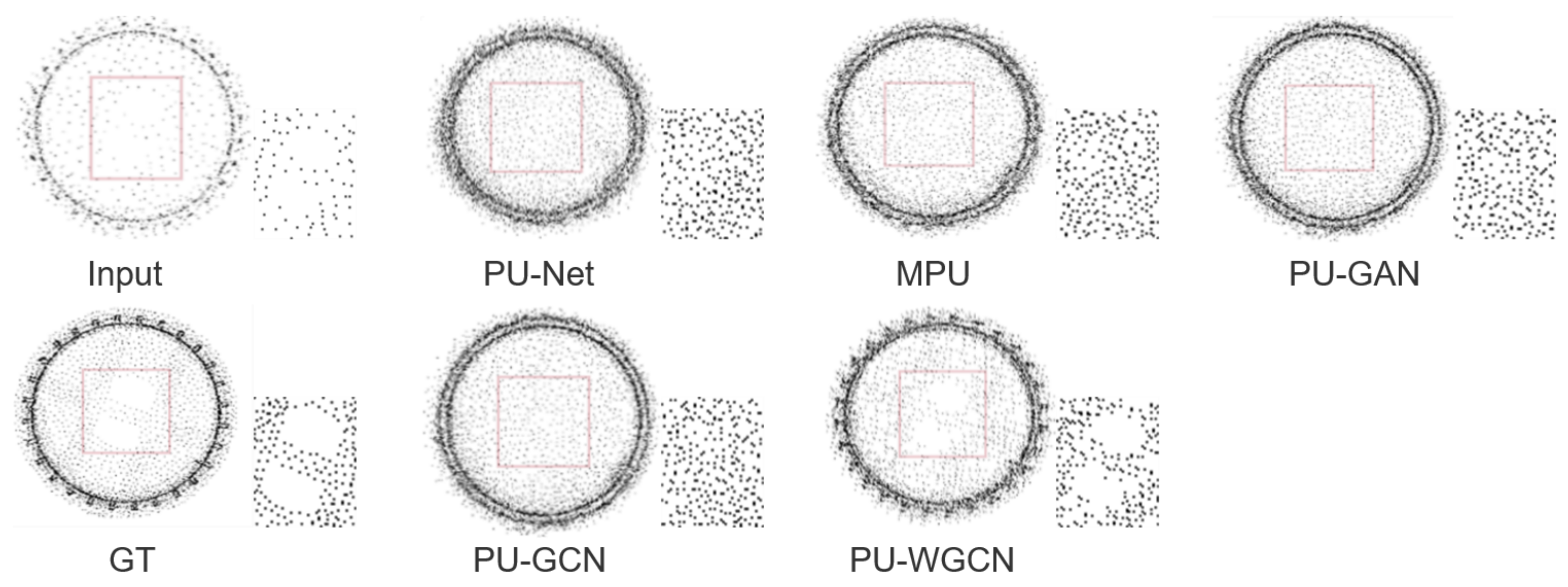
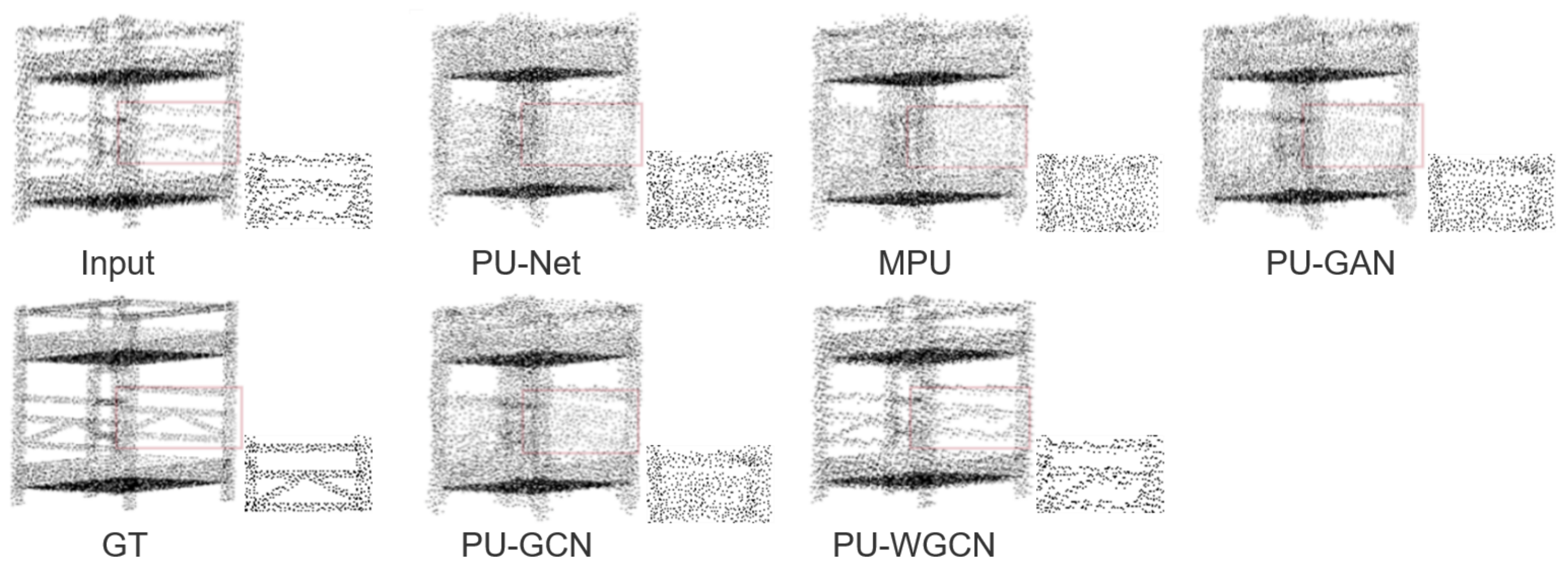
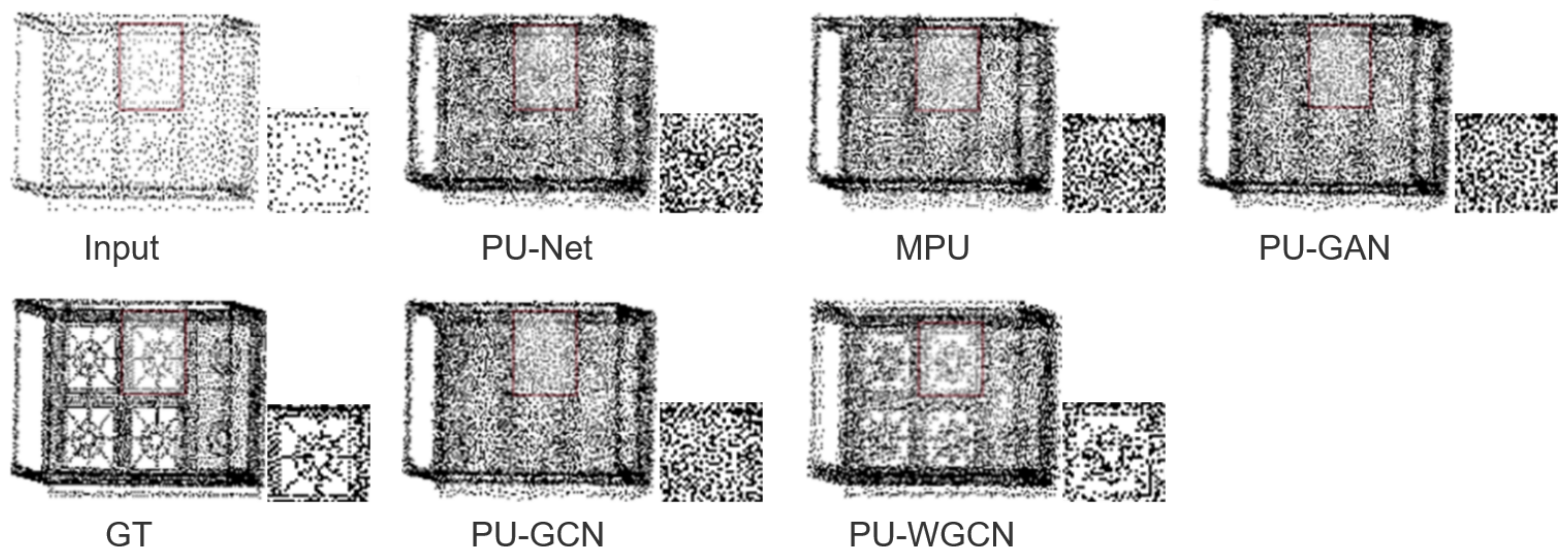
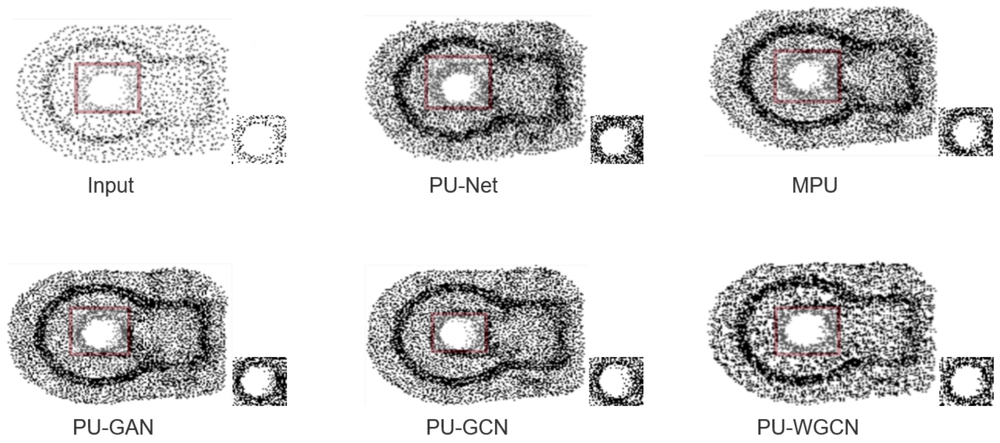
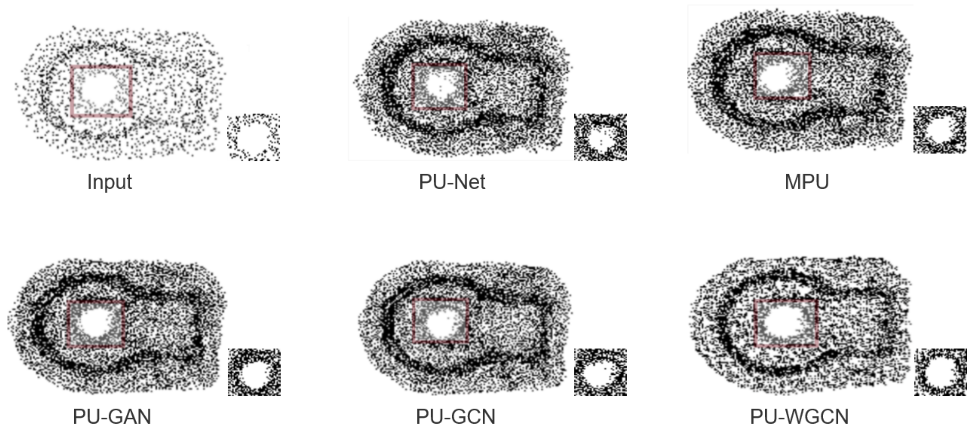
From the data in the table, it is clear that the effect of the upsampling network gradually increases as the number of inputs increases. Comparing this with the data of other groups, the data in Table 4 shows more advanced upsampling effect. We compare the effect of PU-WGCN with PU-Net, MPU, PU-GAN and PU-GCN. All the measures show different degrees of improvement. Among them, CD improved by 0.05 × 10 3 over PU-GCN effect, HD improved by 1.161 × 10 3 over PU-GCN effect, and P2F improved by 0.329 × 10 3 over PU-GCN effect. The experimental results show that our proposed module can focus on the boundary geometry properties of the point clouds, and PU-WGCN can obtain higher-quality upsampled point clouds. In order to visualize the comparative effect of the experiment, we visualize the 3D point cloud model after upsampling. We selected five point cloud models in the test set of pu1k for comparison. The original number of points is 2048. The comparison results are shown in the Figure 11, Figure 12, Figure 13, Figure 14 and Figure 15.
Figure 11, Figure 12, Figure 13, Figure 14 and Figure 15 show the comparison of the effect of PU-WGCN with other upsampling networks. The test data for each network model were obtained from the pu1k dataset. The above figures show the effect of four times the sampling rate, where the number of input points is 2048 and the number of points for GT is 8192. From Figure 11 in group a, it can be seen that the other upsampling networks lose the information of point cloud sawtooths and information of holes. PU-WGCN retains the geometric information of the serrations and the information of the holes. The network upsamples the point cloud of group b, and the blurring problem arises from the strip information of the cabinet sides. The PU-WGCN better preserves the strip geometry information. In group c, we can see the blurring problem at the boundary of the chair. The hole of the chair is also covered by the upsampling points. PU-WGCN retains the information of the chair holes in group c clearly, and the chairs are clearer at the boundaries. In the graph of group d, PU-WGCN can better preserve the information of point cloud boundaries and holes. In group e, the information of point cloud boundaries and holes is almost unrecognizable after upsampling. For PU-WGCN, the information of the holes is retained more completely. The visualization shows that the point cloud model is more complete after upsampling by using PU-WGCN, and the information of its holes and boundaries is better preserved.

4.2. Robustness to Real-Scanned Point Clouds

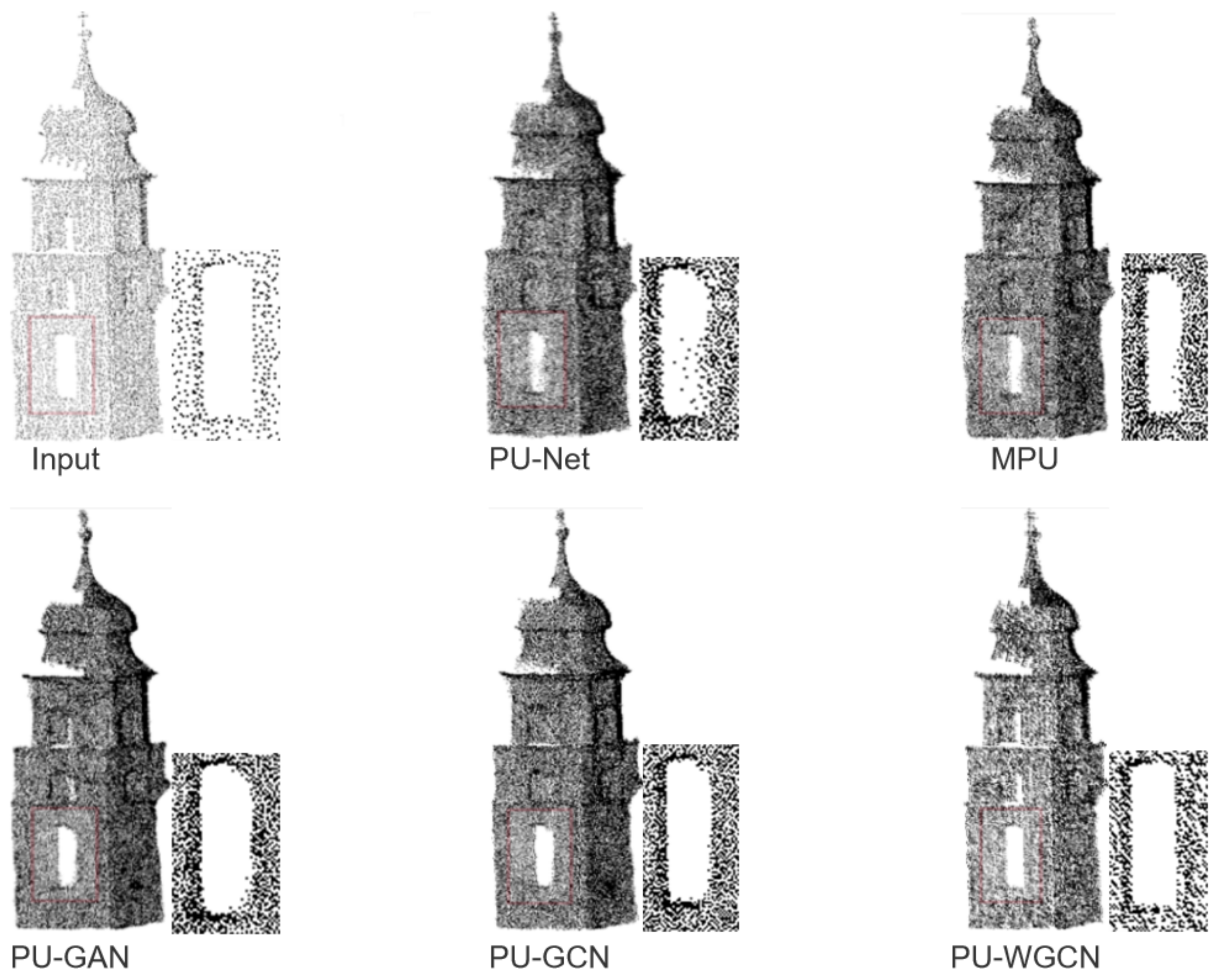
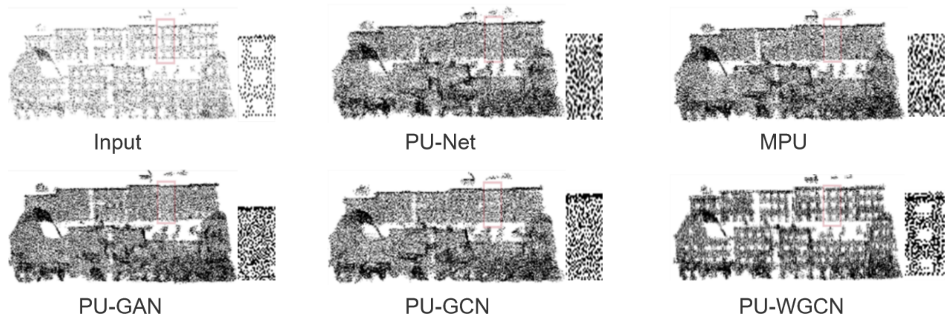
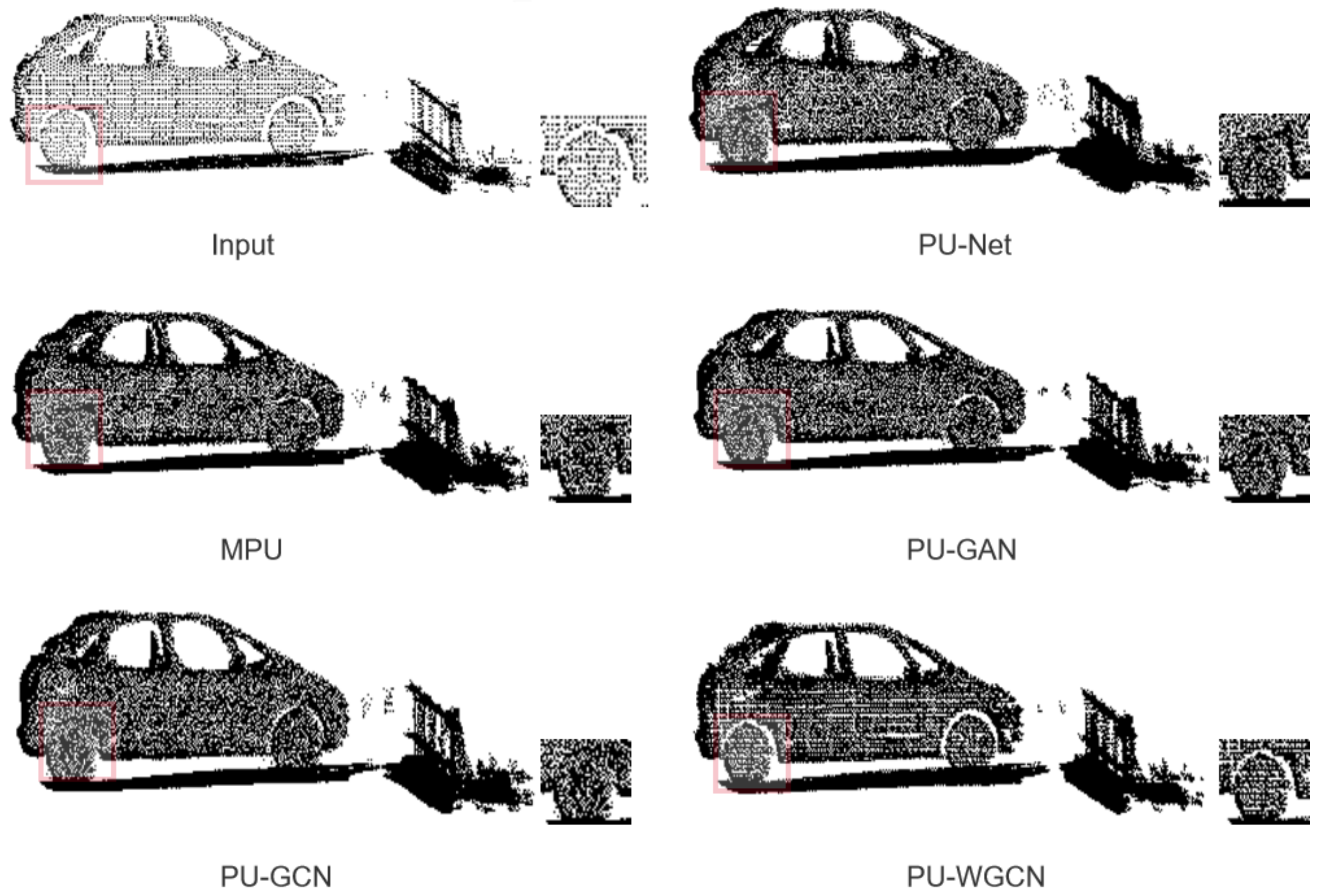
To further verify the upsampling effect of PU-WGCN, we conduct experiments by using real field point clouds. The data used for the network is the point cloud of the city scene in Semantic3D. The comparison effect of each upsampling network is shown in the Figure 16, Figure 17 and Figure 18.
From the visualization figure, we can see that PU-WGCN can retain the boundary information of the input point cloud well, and the holes of the object are also preserved. As shown in Figure 16, the other upsampling networks at the windows of the castle point cloud data in group f appear blurred at the boundaries. PU-WGCN can retain the geometric information of windows very well. PU-WGCN better preserves the window information in group g, while the shape of the window is almost no longer visible in other networks. We upsampled the vehicle point clouds in the h-group roads, and PU-WGCN also expresses significantly better than other networks at details.

4.3. Ablation Study

To compare the effects of the two modules of graph feature enhancement and boundary information weighting, we performed ablation experiments. We select the original GCN, enhanced GCN, weighted boundaries for GCN, and the WGCN for upsampling experiments respectively. We keep the choice of other parameters consistent for all experiments to ensure the accuracy of the results. The dataset for training and testing is pu1k. From the data in Table 1, Table 2, Table 3 and Table 4, it is clear that the best upsampling effect is found in Table 4. Therefore, we selected the PU-GCN in Table 4 for the ablation experiment comparison.
From the experimental results in Table 5, we can see that the HD of the graph feature enhancement module is improved by 1.278 × 10 3 compared to the PU-GCN effect. The CD of the boundary information weighting module is improved by 0.061 × 10 3 and the P2F is improved by 0.255 × 10 3 compared to the PU-GCN effect. Overall, the two modules show different degrees of improvement in the three evaluation metrics.

4.4. Robustness of PU-WGCN

We add Gaussian noise to the input point cloud in order to test the robustness of the network. Figure 19 shows the original point cloud without added noise named casting, which has 2048 points. But here, we just shift the position of the input point cloud instead of adding new points. The effect of upsampling network robustness is shown in the figure. Noise1 in Figure 20 is a Gaussian noise point cloud with a variance of 0.01 added, and Noise2 in Figure 21 is chosen with a variance of 0.02.
As seen in the above figures, the point clouds with Gaussian noises are upsampled through the previous network, and the object appears blurred to different degrees at the holes and boundaries. After the PU-WGCN network, the holes of the casting are retained more completely and their boundaries are clearer.

5. Discussion and Limitation

We tested the upsampling effect based on the pu1k dataset. The values of the evaluation metrics of PU-WGCN are better than other advanced networks significantly. Among them, CD has a 0.05 × 10 3 enhancement effect over PU-GCN, HD has a 1.161 × 10 3 enhancement effect over PU-GCN, and P2F has a 0.329 × 10 3 enhancement effect over PU-GCN. In addition, we perform upsampling experiments on real scanned point clouds in urban scenes, and PU-WGCN can preserve important geometric features such as window boundaries and road boundaries of the original point clouds. PU-WGCN has higher upsampling quality. Despite the above achievements, we did not make use of the geometric topology information of the point cloud. The geometric topology of the point cloud is more expressive of the shape information of the point cloud, which has a facilitating effect on upsampling. In future research work, we hope to use the topological structure information of the point clouds and further obtain better quality upsampled point clouds.

6. Conclusions

In this paper, we analyze the hole overfilling and the boundary blurring problem that occurs with upsampling on point clouds. The feature similarity is too high when the point cloud graph is constructed in the local neighborhood. This is because the neighboring points are close to each other. Moreover, the aggregated neighborhood operation treats all neighboring nodes equally. These two reasons cause the network to overfill the holes of the object when upsampling them. In addition, the current network does not have strict restrictions on the upsampling boundary points. This leads to spillover of point clouds at the boundaries after upsampling, and object boundaries become blurred. To solve the above problem, we propose the PU-WGCN. In this network, we design the weighted graph neural network module (WGCN). This module solves the problem of overfilled holes and blurred boundaries by two operations of enhanced graph features and weighting of boundary information. After experiments, it can be seen that the PU-WGCN network can preserve the hole and boundary geometric properties of the point cloud, and PU-WGCN has effective upsampling.

Author Contributions

Conceptualization, F.G. and C.Z.; methodology, F.G. and C.Z.; software, H.W.; validation, F.G., C.Z. and H.W.; investigation, F.G.; resources, Q.H.; data curation, Q.H., C.Z. and L.H.; writing—original draft preparation, F.G.; writing—review and editing, F.G. and C.Z.; visualization, F.G., C.Z., H.W. and L.H.; supervision, C.Z. and Q.H.; project administration, F.G. and H.W. All authors have read and agreed to the published version of the manuscript.

Funding

This research was funded by the National Natural Science Foundation of China (nos. 62072024 and 41971396), the Projects of Beijing Advanced Innovation Center for Future Urban Design (nos. UDC2019033324 and UDC2017033322), R&D Program of Beijing Municipal Education Commission (KM202210016002 and KM202110016001), the Fundamental Research Funds for Municipal Universities of Beijing University of Civil Engineering and Architecture (nos. X20084 and ZF17061), and the BUCEA Post Graduate Innovation Project (PG2022144).

Institutional Review Board Statement

Not applicable.

Informed Consent Statement

Not applicable.

Data Availability Statement

The dataset generated and analyzed during the current study can be obtained at https://drive.google.com/drive/folders/1k1AR_oklkupP8Ssw6gOrIve0CmXJaSH3 (accessed on 31 May 2022).

Acknowledgments

The authors are thankful to all the personnel who either provided technical support or helped with data collection. We also acknowledge all the reviewers for their useful comments and suggestions.

Conflicts of Interest

The authors declare no conflict of interest.

References

  1. Lv, C.; Lin, W.; Zhao, B. Voxel Structure-based Mesh Reconstruction from a 3D Point Cloud. IEEE Trans. Multimed. 2021, 24, 1815–1829. [Google Scholar] [CrossRef]
  2. Wu, J. A lidar point cloud encryption algorithm based on mobile least squares. Urban Geotech. Investig. Surv. 2019, 5, 110–115. [Google Scholar]
  3. Huang, K.Y.; Tang, J.C.; Zhou, X.J.; Chen, M.Y.; Fang, Y.M.; Lei, Z.Y. Poisson surface reconstruction algorithm based on improved normal orientation. Laser Optoelectron. Prog. 2019, 56, 88–95. [Google Scholar]
  4. Qi, C.R.; Su, H.; Mo, K.C.; Guibas, L.J. PointNet: Deep learning on point sets for 3D classification and segmentation. In Proceedings of the IEEE Conference on Computer Vision and Pattern Recognition (CVPR), Hawaii, HI, USA, 21–26 July 2017. [Google Scholar]
  5. Qi, C.R.; Li, Y.; Hao, S.; Guibas, L.J. PointNet++: Deep hierarchical feature learning on point sets in a metric space. In Proceedings of the Advances in Neural Information Processing Systems, Long Beach, CA, USA, 4–9 December 2017. [Google Scholar]
  6. Hu, Q.Y.; Yang, B.; Xie, L.H.; Rosa, S.; Guo, Y.L.; Wang, Z.H.; Trigoni, N.; Markham, A. RandLA-Net: Efficient Semantic Segmentation of Large-Scale Point Clouds. In Proceedings of the IEEE Conference on Computer Vision and Pattern Recognition (CVPR), Seattle, WA, USA, 13–19 June 2020. [Google Scholar]
  7. Fan, S.Q.; Dong, Q.L.; Zhu, F.H.; LV, Y.S.; Ye, P.J.; Wang, F.Y. SCF-Net: Learning Spatial Contextual Features for Large-Scale Point Cloud Segmentation. In Proceedings of the IEEE Conference on Computer Vision and Pattern Recognition (CVPR), Online, 19–25 June 2021. [Google Scholar]
  8. Nie, Y.Y.; Hou, J.; Han, X.G.; Niesner, M. RfD-Net: Point Scene Understanding by Semantic Instance Reconstruction. In Proceedings of the IEEE Conference on Computer Vision and Pattern Recognition (CVPR), Online, 19–25 June 2021. [Google Scholar]
  9. He, T.; Huang, H.B.; Yi, L.; Zhou, Y.Q.; Wu, C.H.; Wang, J.; Soatto, S. GeoNet: Deep Geodesic Networks for Point Cloud Analysis. In Proceedings of the IEEE Conference on Computer Vision and Pattern Recognition (CVPR), Long Beach, CA, USA, 15–21 June 2019. [Google Scholar]
  10. Yu, L.Q.; Li, X.Z.; Fu, C.W.; Cohen-Or, D.; Heng, P.A. PU-Net: Point cloud upsampling network. In Proceedings of the IEEE Conference on Computer Vision and Pattern Recognition (CVPR), Salt Lake City, UT, USA, 18–21 June 2018. [Google Scholar]
  11. Wang, Y.F.; Wu, S.H.; Huang, H.; Cohen-Or, D.; Sorkine-Hornung, O. Patch-based progressive 3d point set upsampling. In Proceedings of the IEEE Conference on Computer Vision and Pattern Recognition (CVPR), Long Beach, CA, USA, 15–21 June 2019. [Google Scholar]
  12. Li, R.H.; Li, X.Z.; Fu, C.W.; Cohen-Or, D.; Heng, P.A. PU-GAN: A point cloud upsampling adversarial network. In Proceedings of the IEEE/CVF International Conference on Computer Vision (ICCV), Seoul, Korea, 27 October 2019. [Google Scholar]
  13. Qian, Y.; Hou, J.H.; Kwong, S.; He, Y. PUGeo-Net: A geometry-centric network for 3d point cloud upsampling. In Proceedings of the European Conference on Computer Vision (ECCV), Online, 23–28 August 2020. [Google Scholar]
  14. Feng, W.Q.; Li, J.; Cai, H.R.; Luo, X.N.; Zhang, J.Y. Neural Points: Point Cloud Representation with Neural Fields for Arbitrary Upsampling. In Proceedings of the IEEE/CVF Conference on Computer Vision and Pattern Recognition (CVPR), New Orleans, LA, USA, 19–24 June 2022. [Google Scholar]
  15. Qian, G.C.; Abualshour, A.; Li, G.H.; Thabet, A.; Ghanem, B. PU-GCN: Point cloud up sampling using graph convolutional networks. In Proceedings of the IEEE/CVF Conference on Computer Vision and Pattern Recognition (CVPR), Online, 19–25 June 2021. [Google Scholar]
  16. Li, Y.Y.; Bu, R.; Sun, M.C.; Wu, W.; Di, X.H.; Chen, B.Q. PointCNN: Convolution on X-Transformed Points. In Proceedings of the Advances in Neural Information Processing Systems (NIPS), Palais des Congrès de Montréal, Montréal, QC, Canada, 3–8 December 2018. [Google Scholar]
  17. Wu, W.X.; Qi, Z.A.; Li, F.X. PointConv: Deep Convolutional Networks on 3D Point Clouds. In Proceedings of the IEEE/CVF Conference on Computer Vision and Pattern Recognition (CVPR), Seattle, WA, USA, 13–19 June 2020. [Google Scholar]
  18. Liu, Y.C.; Fan, B.; Xiang, S.M.; Pan, C.H. Relation-Shape Convolutional Neural Network for Point Cloud Analysis. In Proceedings of the IEEE/CVF Conference on Computer Vision and Pattern Recognition (CVPR), Long Beach, CA, USA, 15–21 June 2019. [Google Scholar]
  19. Wang, Y.; Sun, Y.B.; Liu, Z.W.; Sarma, S.E.; Bronstein, M.M.; Solomon, J.M. Dynamic Graph CNN for learning on point clouds. ACM Trans. Graph. 2019, 38, 1–12. [Google Scholar] [CrossRef] [Green Version]
  20. Li, G.H.; Mvller, M.A.; Thabet, A.; Ghanem, B. DeepGCNs: Can GCNs Go as Deep as CNNs? In Proceedings of the IEEE International Conference on Computer Vision (ICCV), Seoul, Korea, 27 October 2019. [Google Scholar]
  21. Li, D.L.; Shen, X.; Yu, Y.T.; Guan, H.Y.; Li, J.; Li, D. Building extraction from airborne multi-spectral lidar point clouds based on graph geometric moments convolutional neural networks. Remote Sens. 2020, 12, 3186. [Google Scholar] [CrossRef]
  22. Petar, V.; Guillem, C.; Arantxa, C.; Adriana, R.; Pietro, L.; Yoshua, B. Graph Attention Networks. In Proceedings of the International Conference on Learning Representations, Toulon, France, 24–26 April 2017. [Google Scholar]
  23. Zi, W.J.; Xiong, W.; Chen, H.; Li, J.; Jing, N. SGA-Net: Self-Constructing Graph Attention Neural Network for Semantic Segmentation of Remote Sensing Images. Remote Sens. 2021, 13, 4201. [Google Scholar] [CrossRef]
  24. Huang, W.B.; Rong, Y.; Xu, T.Y.; Sun, F.C.; Huang, J.Z. Tackling Over-Smoothing for General Graph Convolutional Networks. arXiv 2020, arXiv:2008.09864. [Google Scholar]
  25. Wu, S.W.; Sun, F.; Zhang, W.T.; Cui, B. Graph Neural Networks in Recommender Systems: A Survey. ACM Comput. Surv. 2022. [Google Scholar] [CrossRef]
  26. Tian, Q.Y.; Ding, M.; Yang, H.; Yue, C.B.; Zhong, Y.; Du, Z.Z.; Liu, D.Y.; Liu, J.L.; Deng, Y.F. Predicting drug-target affinity based on recurrent neural networks and graph convolutional neural networks. Comb. Chem. High Throughput Screen. 2022, 25, 634–641. [Google Scholar] [CrossRef] [PubMed]
  27. Li, Z.N.; Yang, B.; Liu, D.Y. Distance Similarity Algorithm for Mining Communities from Complex Networks. J. Front. Comput. Sci. Technol. 2011, 5, 336–346. [Google Scholar]
  28. Wang, K.; Guang, H.; Liang, Z.W.; Ye, M.Y. Detecting community in weighted complex network based on similarities. J. Sichuan Univ. Sci. Ed. 2014, 51, 1170–1176. [Google Scholar]
  29. Yu, L.; Li, T.; Zhan, Q.M.; Yu, K. Segmentation of LiDAR point clouds based on similarity measures in multi-dimensional Euclidean Space. Remote Sens. Land Resour. 2014, 26, 31–36. [Google Scholar]
  30. An, Y.J.; Chen, X.X.; Sui, L.C.; Zhou, R.R. A Structural Road Extraction Method Based on Normal Vectors Similarity of Point Clouds. Bull. Surv. Mapp. 2018, 11, 69–72. [Google Scholar]
  31. Kipf, T.N.; Welling, M. Semi-Supervised Classification with Graph Convolutional Networks. In Proceedings of the International Conference on Learning Representations (ICLR), Toulon, France, 24–26 April 2017. [Google Scholar]
  32. Chen, D.; Lin, Y.; Li, W.; Li, P.; Zhou, J.; Sun, X. Measuring and Relieving the Over-smoothing Problem for Graph NeuralNetworks from the Topological View. In Proceedings of the Association for the Advancement of Artificial Intelligence (AAAI), New York, NY, USA, 7–12 February 2020. [Google Scholar]
  33. Kong, K.Z.; Li, G.H.; Ding, M.C.; Wu, Z.X.; Zhu, C.; Ghanem, B.; Taylor, G.; Goldstein, T. Robust Optimization as Data Augmentation for Large-scale Graphs. In Proceedings of the IEEE/CVF Conference on Computer Vision and Pattern Recognition (CVPR), New Orleans, LA, USA, 19–24 June 2022. [Google Scholar]
  34. Asiri, W.; Wang, Q. A New Perspective on “How Graph Neural NetWorks go Beyond Weisfeiler-Lehman?”. In Proceedings of the International Conference on Learning Representations (ICLR), Online, 25–29 April 2022. [Google Scholar]
  35. Shi, W.J.; Rajkumar, R. Point-GNN: Graph Neural Network for 3D Object Detection in a Point Cloud. In Proceedings of the IEEE/CVF Conference on Computer Vision and Pattern Recognition (CVPR), Seattle, WA, USA, 13–19 June 2020. [Google Scholar]
Figure 1. The holes in the chair are overfilled. The red point cloud represents the original point cloud, and the green point cloud represents the point cloud after upsampling. In order to compare the upsampling effect clearly, we use a circle to select the hole part of the chair for magnification.
Remotesensing 14 05356 g001
Figure 2. Feature extraction module using GCN.
Remotesensing 14 05356 g002
Figure 3. Retain the holes in the chair. The green upsampled point cloud covers the holes of the chair. We have to add constraints to the green point cloud so that the hole information of the chair is preserved.
Remotesensing 14 05356 g003
Figure 4. Feature extraction module using enhanced GCN.
Remotesensing 14 05356 g004
Figure 5. Blurring the boundaries of the chair. Where the red point cloud represents the original point cloud and the green point cloud represents the upsampling point cloud. We use the circles to select the boundary part of the chair to magnify.
Remotesensing 14 05356 g005
Figure 6. Pull back the overflow point. The green upsampled point cloud exceeds the boundary of the red original point cloud, and this phenomenon causes the boundary of the chair to be blurred. For easier observation, we use circles for partial magnification.
Remotesensing 14 05356 g006
Figure 7. Preserve the boundaries of the chair. The red point cloud indicates the original point cloud, and we can see the boundary of the chair by magnifying the circle part clearly. However, the green point cloud produced by the previous algorithm blurs the boundary. We pull back the green points that are beyond the boundary to keep the boundary of the chair.
Remotesensing 14 05356 g007
Figure 8. GCN with boundary weighting is used as the feature extraction module.
Remotesensing 14 05356 g008
Figure 9. PU-WGCN architecture. PU-WGCN consists of four parts: patch extraction, enhanced feature extraction, upsampler, and coordinate reconstructor. In the enhanced feature extraction module, we construct the local neighborhood graph using KNN. The red circle and blue circle in the figure indicate the point cloud graphs constructed under different local neighborhoods, respectively. After that, the point cloud graphs are input into GCN* for feature extraction. To make the ablation experiment clearer, we use GCN* to represent the different feature extraction modules.
Remotesensing 14 05356 g009
Figure 10. Feature extraction module using WGCN.
Remotesensing 14 05356 g010
Figure 11. Upsampling visualization results of group a. We show the upsampled results when processed input point clouds by different upsampling networks (PU-Net, MPU, PU-GAN, PU-GCN, and our PU-WGCN). PU-WGCN preserves the hole information of objects.
Remotesensing 14 05356 g011
Figure 12. Upsampling visualization results of group b. Compared to the previous method, our upsampling boundary is clearer. PU-WGCN keeps the boundary information of objects well.
Remotesensing 14 05356 g012
Figure 13. Upsampling visualization results of group c. PU-WGCN preserves the boundary and hole information of the chair well.
Remotesensing 14 05356 g013
Figure 14. Upsampling visualization results of group d. PU-WGCN retains the motorcycle boundary and hole information well.
Remotesensing 14 05356 g014
Figure 15. Upsampling visualization results of group e. PU-WGCN preserves the hole information of objects.
Remotesensing 14 05356 g015
Figure 16. Visualization of the results in real scenes of group f. We show the upsampled results when processed the input point cloud by different upsampling networks (PU-Net, MPU, PU-GAN, PU-GCN and our PU-WGCN).PU-WGCN retains the hole information of the building well.
Remotesensing 14 05356 g016
Figure 17. Visualization of the results in real scenes of group g. We perform upsampling operations on the building data. At the windows of the building, PU-WGCN preserves the hole and boundary information better.
Remotesensing 14 05356 g017
Figure 18. Visualization of the results in real scenes of group h. We perform upsampling operations on the car data. PU-WGCN retains the hole and boundary information of the car well.
Remotesensing 14 05356 g018
Figure 19. Input and GT point cloud.
Remotesensing 14 05356 g019
Figure 20. Robustness test by adding Gaussian noise with a variance of 0.01.
Remotesensing 14 05356 g020
Figure 21. Robustness test by adding Gaussian noise with a variance of 0.02.
Remotesensing 14 05356 g021
Table 1. Comparison of upsampling results for point cloud numbers from 256 to 1024.
NetworkCD 10 3 HD 10 3 P2F 10 3
PU-Net4.56949.43115.645
MPU3.82138.1237.513
PU-GAN3.27431.2607.970
PU-GCN3.18631.8847.724
PU-WGCN2.93629.5677.265
Table 2. Comparison of upsampling results for point cloud numbers from 512 to 2048.
NetworkCD 10 3 HD 10 3 P2F 10 3
PU-Net2.99935.24011.189
MPU2.71729.5678.135
PU-GAN2.08521.8626.949
PU-GCN2.07023.7706.686
PU-WGCN1.91921.7486.014
Table 3. Comparison of upsampling results for point cloud numbers from 1024 to 4096.
NetworkCD 10 3 HD 10 3 P2F 10 3
PU-Net1.88624.3107.407
MPU1.60219.7225.350
PU-GAN1.22314.9324.571
PU-GCN1.14415.5464.312
PU-WGCN1.08713.3513.820
Table 4. Comparison of upsampling results for point cloud numbers from 2048 to 8192.
NetworkCD 10 3 HD 10 3 P2F 10 3
PU-Net1.09214.5614.928
MPU0.94012.5353.459
PU-GAN0.73810.0742.992
PU-GCN0.66910.0872.706
PU-WGCN0.6198.9262.377
Table 5. Experimental results of ablation of point cloud number from 2048 to 8192.
ExperimentsGraph Feature Enhancement ModuleBoundary Information Weighting ModuleCD 10 3 HD 10 3 P2F 10 3
Experiment 1 0.66910.0872.706
Experiment 2 0.6268.8092.550
Experiment 3 0.6089.4582.451
Experiment 40.6198.9262.377
Publisher’s Note: MDPI stays neutral with regard to jurisdictional claims in published maps and institutional affiliations.