Abstract
Ground reference data are typically required to evaluate the quality of a supervised image classification analysis used to produce a thematic map from remotely sensed data. Acquiring a suitable ground data set for a rigorous assessment of classification quality can be a major challenge. An alternative approach to quality assessment is to use a model-based method such as can be achieved with a latent class analysis. Previous research has shown that the latter can provide estimates of class areal extent for a non-site specific accuracy assessment and yield estimates of producer’s accuracy which are commonly used in site-specific accuracy assessment. Here, the potential for quality assessment via a latent class analysis is extended to show that an estimate of a complete confusion matrix can be predicted which allows a suite of standard accuracy measures to be generated to indicate global quality on an overall and per-class basis. In addition, information on classification uncertainty may be used to illustrate classification quality on a per-pixel basis and hence provide local information to highlight spatial variations in classification quality. Classifications of imagery from airborne and satellite-borne sensors were used to illustrate the potential of the latent class analysis with results compared against those arising from the use of a conventional ground data set.
1. Introduction
Ground reference data often play an important role in analyses of remotely sensed imagery. In a standard supervised image classification used in thematic mapping applications, for example, ground data are required normally to train and to test the analysis. Ideally, a ground data set needs to have attributes of quantity and quality as well as properties such as timeliness (i.e., be acquired at a time point close to that of image acquisition) that can be challenging to satisfy. A suitable ground data set can be expensive to acquire, especially if from authoritative field survey. Indeed the expense of traditional field survey is one of the main reasons for using remote sensing as a source of environmental information [1]. Because high quality ground data sets are expensive and challenging to form, means to reduce the training and testing data requirements for image classification have been explored.
The ground data requirements for training a supervised classification analysis can be reduced in a variety of ways. For example, approaches that have been adopted include the use of semi-supervised methods, active learning, historic training sets, pre-trained models with a transfer learning methods, spectral signature libraries, intelligent sample selection, use of data augmentation techniques and of data acquired by crowdsourcing [2,3,4,5,6,7,8]. Critically, however, numerous studies have shown the potential to reduce the training data requirements for accurate supervised image classification.
Ground data are required in the testing stage of a supervised image classification to evaluate the quality of the resulting thematic map and to inform analyses based upon it. The quality of an image classification is typically indicated by an assessment of classification accuracy and/or uncertainty in the labelling of cases in a testing set. Although accuracy and uncertainty are different concepts, with accuracy focused on the degree of error and uncertainty on the confidence of the class labelling, they both provide useful information to evaluate the quality of a thematic map derived from a classification analysis [9,10]. Attention is typically focused on accuracy assessment and the standard approach is a global accuracy assessment based on design-based inference for which recommendations for good practice exist [11]. A core component of the advice is the use of ground data acquired following an appropriate probability sample design. This can be a challenge to satisfy but given the importance of an accuracy assessment it has been suggested that a third of a mapping project’s budget should be allocated to accuracy assessment to enable a rigorous analysis [12]. A map without an accuracy assessment is an untested hypothesis, just one possible representation of the theme that is of ill-defined quality [12]. While the sampling design imposes a constraint that need not apply to training data there are ways to reduce the testing set requirements. The design of the accuracy assessment can, for example, include actions to meet specific mapping objectives and cost constraints [13].
Commonly, most attention is focused on a global assessment of the quality of the thematic map generated by the classification analysis. The latter assessment normally involves the production of an accuracy statement to accompany the map. The central feature of the accuracy statement is typically a summary statistic of overall map quality (e.g., percentage correctly classified cases ideally with confidence intervals at a specified level of significance). Often this reporting may be supplemented with accuracy information for individual classes and the provision of a confusion matrix from which a range of measures of classification quality can be calculated. Thus, for example estimates of accuracy on a per-class basis from the user’s and producer’s perspective may be provided [14]. These latter accuracy indicators are again global, relating to the entire map. However, a global accuracy statement will not convey information on how accuracy varies in space. Classification accuracy may vary geographically, with differences, for example, associated with local variations in the fragmentation of the landscape and image acquisition viewing geometry within the mapped area. Errors are, however, often concentrated spatially especially near inter-class boundaries [15,16,17,18]. Thus, there is sometimes a desire for local information recognising that classification quality can be variable in space [19,20,21,22,23].
Approaches to mapping accuracy locally may, for example, interpolate key measures between ground data sites or constrain the region providing ground data for estimation [9,20,24,25,26,27]. Such approaches, however, may require very considerable ground reference data if the measures are to be of value, especially if to be generated for numerous small sub-regions of the mapped area. An alternative approach to gaining local information on classification quality is to focus on the uncertainty of class allocations. For example, local estimates of classification quality such as per-pixel measures of class labelling uncertainty generated in the analysis may be mapped. Thus, maps of variables such as the posterior probabilities of class membership generated in a conventional maximum likelihood classification can be produced [17,23]. This approach provides a wall-to-wall illustration of classification quality without any ground data for testing purposes.
Often classification quality assessments are undertaken sub-optimally which limits their value. For example, the use of a small testing set in an accuracy assessment may be associated with uncertain estimates (e.g., wide confidence intervals) and use of a non-probability sample greatly limits interpretability. None-the-less ways to reduce the costs and acquire ground data exist. As in the training stage, it may, for example, be possible to use crowdsourced data. An alternative approach which could greatly reduce or potentially remove the need for ground reference data is to adopt a method based on model-based inference [28]. Model based approaches have not been widely used in remote sensing but the potential for both non-site- and site-specific accuracy assessment through a latent class analysis has been highlighted [29].
With a latent class model, the outputs of a set of image classifications are used to make model based estimates of quality measures for each of the input classifications. This is, therefore, a means to intrinsic quality assessment with the quality measures generated directly from the input data themselves. In [29] the focus was on making estimates of the extent of each class in the region mapped, which can be used in non-site specific accuracy assessment, and of the producer’s accuracy, which provides a per-class measure that is widely estimated in conventional site-specific accuracy assessments. Critically, the two measures, class extent and producer’s accuracy, are parameters of the latent class model and are estimated without ground reference data. Here, the aim is to revisit and extend the exploration of the potential of latent class analysis for accuracy assessment. Specifically, this paper seeks to illustrate two key issues. First, that a matrix of conditional probabilities of class membership may be obtained. This matrix shows the pattern of class allocations, correct and errors, for all classes and thus, provides, in essence, information on class allocations similar to a conventional confusion matrix. From this matrix, a range of global measures of accuracy may be calculated on both a per-class and overall basis without any ground reference data. Second, the latent class analysis allows both global and local assessments of classification quality to be undertaken. The latent class analysis can yield estimates of key class allocation probabilities that allow quality to be estimated on a per-pixel basis and enable a wall-to-wall representation of classification quality. Thus, it will be argued that the latent class analysis can provide both local and global assessments of classification quality on both an overall and per-class basis without any ground reference data.
2. Methods
Two remotely sensed data sets acquired for the region around the village of Feltwell in the UK were used. These data have been used and reported on in earlier work (e.g., [4,30]) and hence here only key details are provided. The study area comprised mainly flat land that has been divided up into large agricultural fields and has been used as a test site for a range of remote sensing missions for many years. The remotely sensed data used were acquired by the SPOT HRV [31] and an airborne thematic mapper (ATM) in June and July 1986 respectively. A key attraction of these data sets was the availability of high quality ground data acquired near the time of image acquisitions which showed the crop type planted in most fields in the study area to allow conventional quality assessments to compare against the results from the latent class analyses; the ground data were used only to generate a conventional quality assessment for comparative purposes.
The ATM sensor used acquired data in 11 spectral wavebands. A feature selection analysis indicated that a high degree of class separability could be acquired using only the data acquired in three bands: these were the 0.60–0.63 µm, 0.69–0.75 µm and 1.55–1.75 µm wavebands. Focusing on only the data acquired in these three bands also helped reduce the training data requirements for the six classes that dominated the test site: sugar beet (S), wheat (W), barley (B), carrot (C), potato (P) and grass (G). In an earlier study [30], the ATM data set had been classified using four popular classifiers: a discriminant analysis, a decision tree, a multi-layer perceptron neural network using a backpropagation learning algorithm and a support vector machine with a radial basis function kernel. The new work presented here uses the confusion matrices, generated with a testing set of 320 classified pixels acquired with a simple random sample design, to describe the accuracy of the classifications (reported in Figure 3 of [30]).
The SPOT HRV image (Figure 1) was used mainly to illustrate the ability to generate local information on classification quality. A small image extract (Figure 1b) was used which contains mainly three classes: sugar beet, wheat and barley. The three crop classes in the image extract were highly separable spectrally. However, with 20 m pixels it would be expected that classification error could occur near the boundaries of classes. At these locations mixed pixels may occur and the classifiers used (described below) would, as conventional hard classifiers, act to force a single class label to each pixel. Thus, while pure pixels of the classes, such as found in the central regions of the field, would be expected to be highly separable there is scope for error near boundaries separating fields planted to different classes.
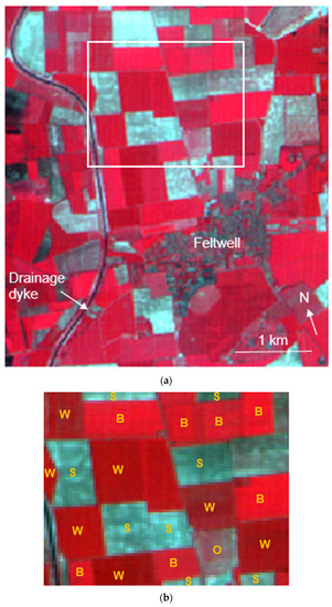
Figure 1.
False colour composite SPOT HRV imagery. (a) regional setting and context around the village of Feltwell, UK. The white box illustrates the extract used to illustrate the potential of latent class analysis for provision of local information on classification quality and (b) the extract used with class labels (B, S and W) annotated; the location labelled O is discussed in the text. Image copyright CNES (2020), reproduced by GMF under licence from SPOT Image.
At the time of the SPOT HRV image acquisition the sugar beet crop would provide only a low amount of ground cover and thus the fields planted to this class would have a spectral response dominated by the background soil and hence have a blue colouration in the false colour composite (Figure 1). While all three classes are spectrally separable in the image, the low ground cover makes the sugar beet class spectrally very dissimilar to the two other crop types. Mixing that involves the sugar beet class might, therefore, result in uncertainty in class membership. Uncertainty in class allocation was, therefore, expected to occur most at inter-class boundaries and especially if the boundary separated sugar beet from another class.
Training data for the three crops were obtained from fields in the region surrounding the image extract. Four classifications were generated by applying minimum distance to means and maximum likelihood classifiers twice, once using just the data in SPOT HRV band 3 and then secondly using the data acquired in all three SPOT HRV wavebands. Note, the focus in this paper is not on producing highly accurate classifications but generating a set that could be used in a latent class analysis.
Latent class modelling has been widely used in other disciplines as a means to estimate the accuracy of a classification when a gold-standard reference data set is unavailable, e.g., [32,33]. In the context of assessing the quality of an image classification, the latent class analysis is focused on the set of class labels for all pixels in the image obtained from the application of a set of different image classifiers. The labels from the set of classifications were used to form a multi-dimensional contingency table that summarized the allocations made and the analysis sought to explain them with a latent variable [34]. Because it is easy to generate multiple classifications of an image, something that is often undertaken if using a consensus approach to classification, it should normally be simple to generate the classification inputs required for a latent class analysis. Indeed the addition of further classifications has the attractive feature of increasing the degrees of freedom in the analysis which helps estimation of parameters from the model [35]. However, this could also result in many cells in the contingency table being empty which can complicate the estimation and interpretation of model fit [36,37]. There is an extensive literature on latent class modelling, e.g., [32,33,34,35,36,37,38,39,40,41] and here only key details are provided for brevity.
The latent class analysis requires that a set of at least three image classifications are available as indicators of the unobserved (latent) variable and its classes [38,39]. In the analysis, the observed associations among the set of classification outputs generated is taken to be explainable by a latent variable that represents the thematic classes of interest [35,39]. The patterns of class labelling observed for the image pixels classified multiple times by the set of classifiers adopted may be used to form a latent class model from which the accuracy of each individual classification may be estimated without the use of ground reference data. The basis of the latent class model for an image data set that has been subjected to four different classification analyses (classifiers A, B, C and D allocating cases to class sets a, b, c, and d respectively), which is the situation for the analyses presented below, is:
where is the probability that a randomly selected case will lie in the a, b, c, d, x cell of the multi-dimensional contingency table, X is the latent variable that has a set of x classes [34,36,40]. The first term or parameter to the right of the equals sign in the latent class model presented in Equation (1), , is the latent class probability which is the probability of a case belonging to class x of the latent variable X. The remaining terms are conditional probabilities that show the probability of a case in class x of the latent variable X belonging to a class as indicated by the relevant input classification. When the latent class and the class allocated by a classification are the same the conditional probability is the producer’s accuracy for that class in the relevant classification. Earlier work in [29] focused on just these two parameters estimated from a latent class analysis (the latent class probability and producer’s accuracy). Here, however, the key focus is on the other conditional probabilities, those for which the classified class label and latent class label differ. These conditional probabilities convey useful information on the pattern of mis-classification.
Information on classification quality may also be generated for each pixel and this may be used to visualize the spatial pattern of classification quality. The set of class allocations made by the classifications together with the parameters of the latent class model allows quantification of the posterior probability of belonging to a class [36,41] using Bayes theorem [36]. This allows each pixel in the image to be allocated to the class with which it displayed the highest posterior probability of membership [36,41]. Critically, this also provides a means to illustrate classification quality on a per-pixel basis. The posterior probabilities may be mapped to illustrate the spatial variation in classification uncertainty. So, beyond the content of [29] it will be stressed that local and global assessments may be undertaken on both overall and per-class basis without ground reference data.
The basic latent class model assumes the input classifications are conditionally independent. This model can, however, be adjusted if conditional dependence is observed which is important to avoid biased estimates of key model parameters [42,43,44]. Here, the latent class modelling was undertaken using the LEM software (obtained from: https://jeroenvermunt.nl/#software, last accessed on 22 October 2022), with model fit assessed with the L2 statistic and conditional dependence was assessed using CONDEP (obtained from: https://www.john-uebersax.com/stat/condep.htm, last accessed on 22 October 2022).
3. Results
As reported in [29], the basic latent class model used appeared to fit with the classifications from the ATM data set, with L2 = 72.3 and no significant conditional dependence observed. The latent classes produced were associated with the crop classes on the basis of prior knowledge of the site, especially class abundance [29]. The latent class and conditional probabilities were output from the analysis for each of the four classifiers applied to the data (Table 1).

Table 1.
Probabilities output from the latent class analysis of the ATM data set. (a) latent class probabilities (i.e., ), (b) conditional probabilities from the discriminant analysis, (c) conditional probabilities from the decision tree, (d) conditional probabilities from the neural network and (e) conditional probabilities from the support vector machine. Note that class membership in the latent variable is shown in columns and the elements on the main diagonal in (b–e) represents the producer’s accuracy.
The output of the latent class model for the ATM data provides information on the land cover classes and their spectral separbility. The probabilities output from the latent class model applied to the ATM data are summarised in Table 1. The probability that a case is a member of a particular latent class, the first term in Equation (1), indicates the abundance or areal extent of the class and the other terms of Equation (1) represent the conditional probabilities. The latent class probability and conditional probability equating to the producer’s accuracy were reported in [29]. For example, the second term in Equation (1) would be the producer’s accuracy for classifier A when the class label in a is the same as that in x. Here, the key focus is on the other conditional probabilities of class membership output from the latent class analysis. These latter probabilities indicate the pattern of class allocation, critically providing information on misclassifications that can aid the evaluation of the quality of a classification and inform other analyses. For example, Table 1b shows the conditional probabilities of class membership generated from the latent class analysis with regard to the classification by the discriminant analysis. This matrix shows patterns of misclassification with non-zero entries in elements off the main diagonal indicating the magnitude of misclassification. For example, in Table 1b it is evident that some cases the latent class analysis associated with the sugar beet (S) class have some confusion with the wheat (W) and potato (P) classes. Specifically P(W|S) = 0.0189 and P(P|S) = 0.0522. Importantly, the conditional probabilities generated from the latent class analysis are close to those obtained with the use of the ground reference data in the available testing set (Table 2). To aid assessment the difference between the individual conditional probabilities are shown in Table 3. Thus not only does the latent class analysis provide information on class abundance that can be used in non-site specific accuracy assessment and the producers’s accuracy for each class it provides information on the pattern of class allocation, critically highlighting misclassifications amongst the classes.
Table 2.
Probabilities of class membership obtained with ground reference data; actual class of membership in columns. Values calculated as conditional to actual class of membership. (a) probability of class occurrence, (b) conditional probabilities from the discriminant analysis, (c) conditional probabilities from the decision tree, (d) conditional probabilities from the neural network and (e) conditional probabilities from the support vector machine. As in Table 1, the main diagonal in (b–e) represents the producer’s accuracy.
Table 3.
Difference between the latent class and actual value determined with ground data (calculated as latent estimate—actual). (a) probability of class occurrence, (b) conditional probabilities from the discriminant analysis, (c) conditional probabilities from the decision tree, (d) conditional probabilities from the neural network and (e) conditional probabilities from the support vector machine.
With information on class abundance, the conditional probabilities of class membership generated from the latent class analysis (Table 1) may be used to generate a prediction of the main content of a full confusion matrix. Thus, the probabilities of the latent class occurrence (Table 1a) may be used with the conditional probabilities generated for each classification analysis (Table 1b–e) to essentially build an estimate of a confusion matrix for each classification which is the basis of numerous measures of classification accuracy. Thus, for example, it has been estimated that 29.94% of the study area is composed of class S (Table 1a). Having the conditional probabilities of membership to each class given membership of class S would allow the formation of a column of a confusion matrix. This can be illustrated simply by assuming a testing sample of 320 cases to allow comparison against the actual confusion matrices, published in [30], based on a testing set of that size acquired by simple random sampling. As the sugar beet class has been estimated to occupy 29.94% of the test site, the column for that class would be expected to contain 95.81 cases; fractional cases would not occur in reality but maintained for illustrative purposes. Focusing on the classification by the discriminant analysis as an example (Table 1b), of those cases, based on the conditional probabilities of class membership (Table 1b), 89.00 would be labelled sugar beet, 1.81 labelled wheat and 5.00 labelled as potato. Repeating such an analysis for each class allows the prediction of the columns of a confusion matrix generated entirely from the latent class analysis and without the aid of any ground reference data (Table 4); the reference data set were used to assess the quality of the estimates obtained from the latent class analysis. For comparative purposes the actual confusion matrices generated with the 320 testing cases, and published in [30], are shown in Table 5. It is evident that there are differences, which is expected as there are, for instance, differences in the class area estimates from the latent class analysis (Table 1a) and that generated from the ground data (Table 2a), but they are small (Table 3a). Critically, however, an estimate of a full confusion matrix that, while imperfect, illustrates the general pattern of misallocation was obtained from the latent class analysis
Table 4.
Confusion matrices predicted from the outputs from the latent class analysis. (a) for the discriminant analysis, (b) for the decision tree, (c) for the neural network and (d) for the support vector machine.
Table 5.
Confusion matrices generated with the ground reference data; actual class of membership shown in the columns. (a) for the discriminant analysis, (b) for the decision tree, (c) for the neural network and (d) for the support vector machine. Data from [30].
Four classifications of the SPOT HRV data were generated. A latent class analysis assuming conditional independence of the input data, as used with the ATM data, was applied to the four classifications of the SPOT HRV image. As many elements of the multi-dimensional contingency table summarizing the class allocations made by the set of classifiers were associated with zero values the assessment of fit is, however, difficult but the model fitted the data with L2 = 1684.15. Additionally, a test for conditional dependence indicated that was significant dependence between classifications generated by the minimum distance and maximum likelihood classifications that only used the data acquired in SPOT HRV band 3. Informed by this analysis, a series of trials of other models was undertaken. Here, attention focused on a model that includes conditional dependence between the minimum distance and maximum likelihood classifications generated using the same set of spectral wavebands. This model appeared to fit the data more closely than the basic model with L2 = 730.22 although interpretation of the fit statistics is again limited by the large number of elements in the multi-dimensional contingency table with zero values.
4. Discussion
A key outcome from the analyses of the ATM data set was the ability to obtain information on classification accuracy and the pattern of mis-classification. The matrix formed for each classifer (Table 4) has some similarity to a confusion matrix, although representing an imperfect guide to reality. Critically, the matrices may be used to generate a suite of global measures of classification quality on an overall and on a per-class basis (e.g., [14]). For example, the confusion matrix would allow an estimate of the overall proportion of correct allocations (i.e., overall accuracy) or per-class accuracy from the user’s and producer’s perspectives to be generated. The latent class analysis, therefore, provides a means to generate an estimate of traditional global measures of classification accuracy, on an overall and per-class basis without the use of a testing set of ground reference data.
The potential to extract additional and critically local information on classification quality was explored with the SPOT HRV data set. The outputs from the latent class model applied to the four classifications of the SPOT HRV data provide a means to explore the potential for local information on classification accuracy that is available on a wall-to-wall basis. This was illustrated by focusing on locations that may be expected to be associated with uncertainty in class membership in the image extract (Figure 1b).
Figure 2 shows the posterior probabilities generated from the latent class analysis of the region. Note that most pixels have probability values close to 0 or 1. This situation arises because the classes are spectrally separable and so pixels, especially those located in the central or core area of fields, are typically associated very strongly with one class and minimally with the others. A key exception to this situation is near field boundaries where probabilities of an intermediate value were observed. In particular, probabilities of intermediate value were, as expected, often observed with boundaries that separated a field of sugar beet from another class. There is also a region with intermediate posterior probabilities highlighted with an O in Figure 1b. Unfortunately the actual class membership of this region is unknown but visual interpretation of the false colour image (Figure 2a) suggests that while this region has low vegetation cover it has more than typically observed for the sugar beet class. Hence, the region spectrally lies between sugar beet and the other classes, resulting in the analysis yielding posterior probabilities with intermediate values. Critically, the output from the latent class analysis is providing information on classification quality for each pixel, indicating classification quality locally and on a wall-to-wall basis. Consequently, the latent class analysis is providing both local and global information on classification quality.
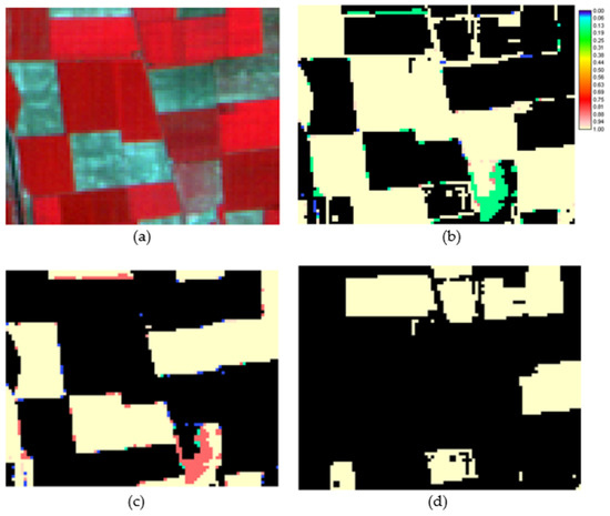
Figure 2.
Spatial information on class allocation quality generated from the latent class analysis. (a) false colour SPOT HRV image of test site, (b) posterior probability to wheat, (c) posterior probability to sugar beet and (d) posterior probability to barley. Image copyright CNES (2020), reproduced by GMF under licence from SPOT Image.
Finally, the results also illustrate a common challenge in quality assessments of image classifications. Note, for instance, that the drainage dyke (Figure 1b) is, in effect, an untrained class but is confidently allocated to one of the set of defined classes (Figure 2). The effect of an underpinning assumption, namely that the set of classes is exhaustively defined, should not be ignored. None-the-less, the latent class analysis appears to offer considerable potential to aid analyses of classifications of remotely sensed data and further, more rigorous, evaluation of the potential of the approach would be valuable. For example, issues such as the number and variety of classifiers used, the effect of deviations from model assumptions, the integration of limited ground data into the analysis and inclusion of probabilities conditional on the matrix’s row as well as column values (i.e. making a better estimate of a confusion matrix) may be topics worthy of exploration.
5. Conclusions
Previous work [29] indicated the potential of latent class analysis for non-site and site-specific accuracy assessment in the form of estimates of class areal extent and producer’s accuracy. The focus had also been on only global assessments of classification accuracy. Here, the potential of latent class modelling has been further assessed. The results reported here show that the latent class model outputs can include a full set of class conditional probabilities, which estimate a full confusion matrix from which numerous global measures of accuracy can be produced. Thus, without ground data, it would be possible to generate estimates of standard measures of global accuracy on an overall basis (e.g., overall accuracy or percent correct) and on a per-class basis from both the user’s and producer’s perspectives. It should be noted, however, that the confusion matrices derived were in close but not perfect agreement to real confusion matrices generated using ground reference data.
In addition to the global information on classification accuracy, it is stressed that information on classification quality was generated for each pixel. Thus, highly localised, per-pixel, information on classification quality can be generated. This was illustrated by focusing on the magnitude of the posterior probabilities of class membership near boundary regions which are known to be a common source of error and uncertainty in image classification analyses. Critically, the latent class analysis was able to provide both local and global information on classification quality on both an overall and per-class basis without use of a testing set. While the examples presented here have been based on conventional per-pixel classifiers the method would be applicable to classifications based on a different spatial unit (e.g., object or field). Further research to more fully and rigorously evaluate the potential of latent class modelling in remote sensing applications, including limitations, would be valuable.
Funding
This research received no external funding.
Data Availability Statement
The SPOT HRV data were acquired via the NERC Earth Observation Data Centre while the ATM and ground data had been acquired as part of the European Commission’s AgriSAR campaign. These data may be available to others from these bodies.
Acknowledgments
I am grateful to the providers of the software and data used. The work has benefitted from research with a range of collaborators in the past although responsibility for all the new work and interpretations lies with G.M.F. I am grateful for the comments from the three referees that helped enhance this article.
Conflicts of Interest
The author declares no conflict of interest.
References
- Lechner, A.M.; Foody, G.M.; Boyd, D.S. Applications in remote sensing to forest ecology and management. One Earth 2020, 2, 405–412. [Google Scholar] [CrossRef]
- Bruzzone, L.; Chi, M.; Marconcini, M. A novel transductive SVM for semisupervised classification of remote-sensing images. IEEE Trans. Geosci. Remote Sens. 2006, 44, 3363–3373. [Google Scholar] [CrossRef]
- Saha, S.; Mou, L.; Zhu, X.X.; Bovolo, F.; Bruzzone, L. Semisupervised change detection using graph convolutional network. IEEE Geosci. Remote Sens. Lett. 2021, 18, 607–611. [Google Scholar] [CrossRef]
- Foody, G.M.; Mathur, A. Toward intelligent training of supervised image classifications: Directing training data acquisition for SVM classification. Remote Sens. Environ. 2004, 93, 107–117. [Google Scholar] [CrossRef]
- Li, X.; Zhang, L.; Du, B.; Zhang, L.; Shi, Q. Iterative reweighting heterogeneous transfer learning framework for supervised remote sensing image classification. IEEE J. Sel. Top. Appl. Earth Obs. Remote Sens. 2017, 10, 2022–2035. [Google Scholar] [CrossRef]
- He, X.; Chen, Y. Transferring CNN ensemble for hyperspectral image classification. IEEE Geosci. Remote Sens. Lett. 2000, 18, 876–880. [Google Scholar] [CrossRef]
- Zhang, J.; He, Y.; Yuan, L.; Liu, P.; Zhou, X.; Huang, Y. Machine learning-based spectral library for crop classification and status monitoring. Agronomy 2019, 9, 496. [Google Scholar] [CrossRef]
- Saralioglu, E.; Gungor, O. Crowdsourcing-based application to solve the problem of insufficient training data in deep learning-based classification of satellite images. Geocarto Int. 2022, 37, 5433–5452. [Google Scholar] [CrossRef]
- Khatami, R.; Mountrakis, G.; Stehman, S.V. Mapping per-pixel predicted accuracy of classified remote sensing images. Remote Sens. Environ. 2017, 191, 156–167. [Google Scholar] [CrossRef]
- Mountrakis, G.; Xi, B. Assessing reference dataset representativeness through confidence metrics based on information density. ISPRS J. Photogramm. Remote Sens. 2013, 78, 129–147. [Google Scholar] [CrossRef]
- Olofsson, P.; Foody, G.M.; Herold, M.; Stehman, S.V.; Woodcock, C.E.; Wulder, M.A. Good practices for estimating area and assessing accuracy of land change. Remote Sens. Environ. 2014, 148, 42–57. [Google Scholar] [CrossRef]
- Strahler, A.H.; Boschetti, L.; Foody, G.M.; Friedl, M.A.; Hansen, M.C.; Herold, M.; Mayaux, P.; Morisette, J.T.; Stehman, S.V.; Woodcock, C.E. Global Land Cover Validation: Recommendations for Evaluation and Accuracy Assessment of Global Land Cover Maps; European Communities: Luxembourg, 2006; Volume 51, pp. 1–60. Available online: https://op.europa.eu/en/publication-detail/-/publication/52730469-6bc9-47a9-b486-5e2662629976 (accessed on 22 October 2022).
- Stehman, S.V. Sampling designs for accuracy assessment of land cover. Int. J. Remote Sens. 2009, 30, 5243–5272. [Google Scholar] [CrossRef]
- Liu, C.; Frazier, P.; Kumar, L. Comparative assessment of the measures of thematic classification accuracy. Remote Sens. Environ. 2007, 107, 606–616. [Google Scholar] [CrossRef]
- Congalton, R.G. Using spatial autocorrelation analysis to explore the errors in maps generated from remotely sensed data. Photogramm. Eng. Remote Sens. 1988, 54, 587–592. [Google Scholar]
- Edwards, G.; Lowell, K.E. Modeling uncertainty in photointerpreted boundaries. Photogramm. Eng. Remote Sens. 1996, 62, 377–390. [Google Scholar]
- Steele, B.M.; Winne, J.C.; Redmond, R.L. Estimation and mapping of misclassification probabilities for thematic land cover maps. Remote Sens. Environ. 1998, 66, 192–202. [Google Scholar] [CrossRef]
- Fuller, R.M.; Groom, G.B.; Jones, A.R. The land-cover map of Great Britain: An automated classification of Landsat thematic mapper data. Photogramm. Eng. Remote Sens. 1994, 60, 553–562. [Google Scholar]
- Meyer, H.; Pebesma, E. Machine learning-based global maps of ecological variables and the challenge of assessing them. Nat. Commun. 2022, 13, 2208. [Google Scholar] [CrossRef]
- Foody, G.M. Local characterization of thematic classification accuracy through spatially constrained confusion matrices. Int. J. Remote Sens. 2005, 26, 1217–1228. [Google Scholar] [CrossRef]
- Mitchell, P.J.; Downie, A.L.; Diesing, M. How good is my map? A tool for semi-automated thematic mapping and spatially explicit confidence assessment. Environ. Model. Softw. 2018, 108, 111–122. [Google Scholar] [CrossRef]
- Bogaert, P.; Waldner, F.; Defourny, P. An information-based criterion to measure pixel-level thematic uncertainty in land cover classifications. Stoch. Environ. Res. Risk Assess. 2017, 31, 2297–2312. [Google Scholar] [CrossRef]
- Foody, G.M.; Campbell, N.A.; Trodd, N.M.; Wood, T.F. Derivation and applications of probabilistic measures of class membership from the maximum-likelihood classification. Photogramm. Eng. Remote Sens. 1992, 58, 1335–1341. [Google Scholar]
- Comber, A.; Fisher, P.; Brunsdon, C.; Khmag, A. Spatial analysis of remote sensing image classification accuracy. Remote Sens. Environ. 2012, 127, 237–246. [Google Scholar] [CrossRef]
- Comber, A.; Brunsdon, C.; Charlton, M.; Harris, P. Geographically weighted correspondence matrices for local error reporting and change analyses: Mapping the spatial distribution of errors and change. Remote Sens. Lett. 2017, 8, 234–243. [Google Scholar] [CrossRef]
- Comber, A.J. Geographically weighted methods for estimating local surfaces of overall, user and producer accuracies. Remote Sens. Lett. 2013, 4, 373–380. [Google Scholar] [CrossRef]
- Ebrahimy, H.; Mirbagheri, B.; Matkan, A.A.; Azadbakht, M. Per-pixel land cover accuracy prediction: A random forest-based method with limited reference sample data. ISPRS J. Photogramm. Remote Sens. 2021, 172, 17–27. [Google Scholar] [CrossRef]
- McRoberts, R.E.; Naesset, E.; Gobakken, T. Accuracy and precision for remote sensing applications of nonlinear model-based inference. IEEE J. Sel. Top. Appl. Earth Obs. Remote Sens. 2013, 6, 27–34. [Google Scholar] [CrossRef]
- Foody, G.M. Latent class modeling for site-and non-site-specific classification accuracy assessment without ground data. IEEE Trans. Geosci. Remote Sens. 2012, 50, 2827–2838. [Google Scholar] [CrossRef]
- Foody, G.M.; Mathur, A. A relative evaluation of multiclass image classification by support vector machines. IEEE Trans. Geosci. Remote Sens. 2004, 42, 1335–1343. [Google Scholar] [CrossRef]
- Lillesand, T.; Kiefer, R.W.; Chipman, J. Remote Sensing and Image Interpretation, 7th ed.; John Wiley & Sons: New York, NY, USA, 2015. [Google Scholar]
- Collins, J.; Huynh, M. Estimation of diagnostic test accuracy without full verification: A review of latent class methods. Stat. Med. 2014, 33, 4141–4169. [Google Scholar] [CrossRef]
- Garrett, E.S.; Eaton, W.W.; Zeger, S. Methods for evaluating the performance of diagnostic tests in the absence of a gold standard: A latent class model approach. Stat. Med. 2002, 21, 1289–1307. [Google Scholar] [CrossRef]
- McCutcheon, A.L. Latent Class Analysis; Sage: Newbury Park, CA, USA, 1987. [Google Scholar]
- Yin, Z.G.; Zhang, J.B.; Kan, S.L.; Wang, X.G. Diagnostic accuracy of imaging modalities for suspected scaphoid fractures: Meta-analysis combined with latent class analysis. J. Bone Jt. Surgery Br. Vol. 2012, 94, 1077–1085. [Google Scholar] [CrossRef]
- Vermunt, J.K.; Magidson, J. Latent class analysis. In The SAGE Encyclopedia of Social Sciences Research Methods; Lewis-Beck, M.S., Bryman, A., Liao, T.F., Eds.; Sage: Thousand Oaks, CA, USA, 2004; pp. 549–553. [Google Scholar]
- van Kollenburg, G.H.; Mulder, J.; Vermunt, J.K. Assessing model fit in latent class analysis when asymptotics do not hold. Methodol. Eur. J. Res. Methods Behav. Soc. Sci. 2015, 11, 65–79. [Google Scholar] [CrossRef][Green Version]
- Rutjes, A.W.S.; Reitsma, J.B.; Coomarasamy, A.; Khan, K.S.; Bossuyt, P.M.M. Evaluation of Diagnostic Tests when There Is no Gold Standard. A Review of Methods. Health Technol. Assess. 2007, 11. [Google Scholar] [CrossRef]
- Walter, S.D. Estimation of diagnostic test accuracy: A “Rule of Three” for data with repeated observations but without a gold standard. Stat. Med. 2021, 40, 4815–4829. [Google Scholar] [CrossRef]
- Yang, I.; Becker, M.P. Latent variable modeling of diagnostic accuracy. Biometrics 1997, 53, 948–958. [Google Scholar] [CrossRef]
- Magidson, J.; Vermunt, J.K. Latent class models. In The SAGE Handbook of Quantitative Methodology for the Social Sciences; Kaplan, D., Ed.; Sage: Thousand Oaks, CA, USA, 2004; pp. 175–198. [Google Scholar]
- Albert, P.S.; Dodd, L.E. A cautionary note on the robustness of latent class models for estimating diagnostic error without a gold standard. Biometrics 2004, 60, 427–435. [Google Scholar] [CrossRef]
- Pepe, M.S.; Janes, H. Insights into latent class analysis of diagnostic test performance. Biostatistics 2007, 8, 474–484. [Google Scholar] [CrossRef]
- Visser, M.; Depaoli, S. A guide to detecting and modeling local dependence in latent class analysis models. Struct. Equ. Model. Multidiscip. J. 2022, 1–12. [Google Scholar] [CrossRef]


Publisher’s Note: MDPI stays neutral with regard to jurisdictional claims in published maps and institutional affiliations. |
© 2022 by the author. Licensee MDPI, Basel, Switzerland. This article is an open access article distributed under the terms and conditions of the Creative Commons Attribution (CC BY) license (https://creativecommons.org/licenses/by/4.0/).