Abstract
The enormous increase in the volume of Earth Observations (EOs) has provided the scientific community with unprecedented temporal, spatial, and spectral information. However, this increase in the volume of EOs has not yet resulted in proportional progress with our ability to forecast agricultural systems. This study examines the applicability of EOs obtained from Sentinel-2 and Landsat-8 for constraining the APSIM-Maize model parameters. We leveraged leaf area index (LAI) retrieved from Sentinel-2 and Landsat-8 NDVI (Normalized Difference Vegetation Index) to constrain a series of APSIM-Maize model parameters in three different Bayesian multi-criteria optimization frameworks across 13 different calibration sites in the U.S. Midwest. The novelty of the current study lies in its approach in providing a mathematical framework to directly integrate EOs into process-based models for improved parameter estimation and system representation. Thus, a time variant sensitivity analysis was performed to identify the most influential parameters driving the LAI (Leaf Area Index) estimates in APSIM-Maize model. Then surrogate models were developed using random samples taken from the parameter space using Latin hypercube sampling to emulate APSIM’s behavior in simulating NDVI and LAI at all sites. Site-level, global and hierarchical Bayesian optimization models were then developed using the site-level emulators to simultaneously constrain all parameters and estimate the site to site variability in crop parameters. For within sample predictions, site-level optimization showed the largest predictive uncertainty around LAI and crop yield, whereas the global optimization showed the most constraint predictions for these variables. The lowest RMSE within sample yield prediction was found for hierarchical optimization scheme (1423 Kg ha) while the largest RMSE was found for site-level (1494 Kg ha). In out-of-sample predictions for within the spatio-temporal extent of the training sites, global optimization showed lower RMSE (1627 Kg ha) compared to the hierarchical approach (1822 Kg ha) across 90 independent sites in the U.S. Midwest. On comparison between these two optimization schemes across another 242 independent sites outside the spatio-temporal extent of the training sites, global optimization also showed substantially lower RMSE (1554 Kg ha) as compared to the hierarchical approach (2532 Kg ha). Overall, EOs demonstrated their real use case for constraining process-based crop models and showed comparable results to model calibration exercises using only field measurements.
1. Introduction
Data ingestion and data integration are grand challenges of today’s age of digital agriculture. The enormous volume of data produced by all phases of agriculture, such as field observations, satellite imagery, flux towers or soil/plant sensors, has enabled data-driven decision making for improving agricultural productivity [1,2,3]. However, the inherently fragmented nature of observational data due to variable temporal and/or spatial resolution has made the integration of these data products challenging and often impractical [4]. As a result, previous multidimensional assessments of agricultural productivity and environmental impacts have often fallen short of data-measured potential. To perform multidimensional studies across broads regions, agricultural researchers are increasingly turning to process-based simulation models [5,6], such as the The Agricultural Production Systems sIMulator (APSIM) [7] or the Decision Support System for Agrotechnology Transfer (DSSAT) [8]. These models integrate state-of-the-art knowledge on a multitude of soil and crop processes to enable analyses of higher dimensionality than what is possible with field experiments. These pioneering models are at the core of many recent forecasting and climate impact assessment efforts around the world [9,10,11]. However, due to the large number of uncertain parameters within these models, their predictive capacity is limited in accuracy, precision, or both for real-world applications [12,13].
Although constraining parameters in nonlinear models is a common task across many different disciplines, optimizing and constraining process-based crop model parameters is a particularly challenging task for several reasons [14]. First, process-based crop models are computationally expensive, and it is often impractical to optimize them using “big data” that spans a large number of sites and/or years [15]. As a result, crop model calibration exercises are typically limited to a single site or single data constraint, an approach that is in direct contrast to the diverse range of available observations produced by all phases of agriculture [13]. Second, the observational data used for calibrating crop models often have substantial associated uncertainty due to low sample size. Since most numerical optimization techniques lack mechanisms to account for uncertainty in observational data, their application can potentially lead to wrongly over-confident model predictions. Third, it is unclear how observational data from multiple sites and years can be simultaneously ingested. The most common approach is to independently calibrate crop models at different sites (known as site-level calibration); however, this approach assumes that all sites are completely independent and ignores the potential of across-site information. Consequently, site-level calibration offers limited potential for upscaling model simulations to new sites and across broad regions [15,16]. On the other hand, global optimization (known as joint calibration) assumes no site-to-site variability and pools all observations to identify a combination of parameters that minimizes model prediction error at all sites simultaneously. Past studies have shown that both approaches have trouble estimating the “true” uncertainty in model parameters and offer no formal distinction between “within-sample” prediction and “out-of-sample” prediction [17]. In addition, these approaches provide no clear path to capturing spatiotemporal variability in model parameters. Lastly, process-based models are calibrated with a limited number of observations that often pales in comparison to the potential list of parameters impacting the simulated results. This often results in equifinality, such that calibration does not lead to unique parameter values and different combinations of parameter values can give the same results [14]. Due to the above-mentioned reasons, most model calibration studies lack proper constraint and accounting of uncertainty in model parameters and, therefore, produce models that perform well only in a subspace of the genetics (G), environment (E), and management (M) (G × E × M) inference space and, consequently, have limited generalizability for broader applications.
Earth Observations (EOs) with their extensive temporal and spatial coverage have provided the scientific community with a unique opportunity to monitor and map plant status [18]. Radiative Transfer Models (RTM) have enabled retrieval of biophysical and biochemical plant traits from EOs through both passive and active measurements [19,20]. These estimates are spatially contiguous and temporally frequent and they offer a substantially larger sample size compared to field measurements [21]. Consistent and long-term plant traits obtained from EOs could potentially inform process-based models, constraining multiple state variables, such as LAI, plant N concentration, and plant biomass, and/or model parameters, such as thermal times for phenological stages. Thus, EOs could help to overcome the spatiotemporal limitations of field experiment data and could serve as a powerful resource for multi-criteria crop model calibration across broad regions [21]. However to leverage EOs, novel and flexible methods are needed that allow for streamlining data extraction, ingestion, and integration into crop models with the goal of constraining model parameters and state variables.
As one of the most widely used process-based crop models, APSIM model has been calibrated using a variety of different optimization techniques and observational data types for simulating maize across the U.S. Midwest [22,23,24,25]. These studies have often achieved high yet inconsistent prediction accuracy in estimating maize grain yields. For instance, ref. [26] tested the APSIM model with 12 years of experimental data covering maize-maize and maize-soybean rotations in IA. APSIM captured changes in maize yield due to nitrogen fertilizer treatments but still made large prediction errors in a few site-years. The authors attributed such errors to missing crop damage processes (i.e., hail), missing spatial information (i.e., elevation), and an overly simple N-uptake routine, which emphasized N stress at floral initiation. Ref. [27] also calibrated and tested APSIM at several maize sites in the state of Iowa in the U.S. and found the model to be highly accurate, explaining 87% of the variability in maize yields and achieving a Normalized Root Mean Square Error (nRMSE) value of 7.7%. However, the authors also highlighted the fact that their calibration and validation datasets originated from a similar study area and, consequently, experienced the same weather patterns. Consequently, their calibrated model was tested under limited environmental conditions. Ref. [24] calibrated APSIM for 6 years of experimental data covering maize-maize, maize-soybean, and winter cover crop rotations in IA to investigate crop water use efficiency. When performing two-year simulations, they found the model was successful in predicting yield for the maize-maize rotations with an RMSE of 723 kg/ha. Ref. [28] calibrated the APSIM model for 16 site-years in the U.S. Midwest that spanned different rotations and fertilizer rates. They found the calibrated model to perform better when N fertilizers were applied since the model only had to rely on correct water limitation simulation. Moreover, ref. [29] used default APSIM settings to test the model in predicting maize stover and grain yield at three locations. Against 113 observations, APSIM achieved an RMSE of 1241 kg/ha (nRMSE 14%) for maize grain yield estimates, and the authors also noted improved simulation with increased N fertilizer rates (i.e., lower N stress conditions).
Although the APSIM model has been calibrated and validated extensively using field observations, the unprecedented data coverage provided by EOs has never been leveraged to our knowledge to optimize APSIM and broaden its successful application. In this study, we present a mathematical framework that constrains APSIM model parameters with EOs for maize simulations in the U.S. Midwest using emulation and three Bayesian optimization schemes: global, individual, and hierarchical. The overall objectives of the current study are: (1) to assess the potential of EOs for improving maize yield prediction using the APSIM model; and (2) to compare different optimization techniques with varying degrees of information sharing across sites in their maize yield prediction in the U.S. Midwest.
2. Materials and Methods
2.1. Overall Workflow
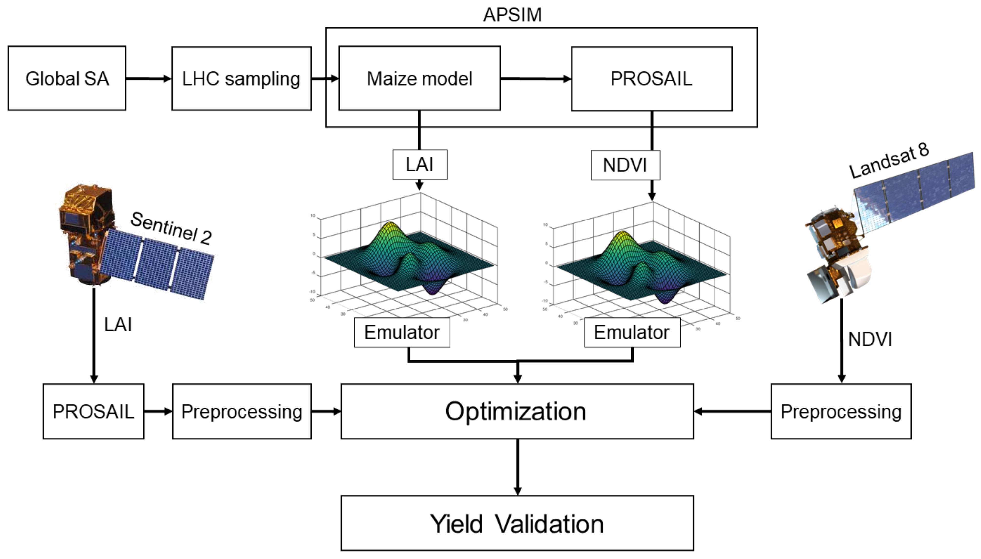
This study explores the effectiveness of incorporating EOs into the APSIM crop model through different optimization schemes to constrain and improve maize yield prediction (Figure 1). First, a comprehensive global sensitivity analysis (GSA) was performed to identify the most influential parameters controlling LAI estimation. Next, APSIM was run across a series of random parameter samples drawn from the influential parameter space at 13 calibration sites. Based on these runs, surrogate models (emulators) were developed using Generalized Additive Models (GAMs) to replace APSIM with more efficient statistical models. These GAMS were trained on the model output to estimate LAI and Normalized Difference Vegetation Index (NDVI) at each site as a function of influential parameters. LAI estimates from Sentinel-2 and NDVI estimates from Landsat-8 were then used to constrain the model parameters using the fitted site-level emulators within a Bayesian optimization framework. Finally, the information contribution of the LAI and NDVI observations was assessed in simulating maize yield across different optimization schemes and 332 sites in the U.S. Midwest.

Figure 1.
The overall workflow of linking APSIM-Maize model with radiative transfer model (PROSAIL) for developing the emulators, optimization procedure and model validation.
2.2. Study Sites
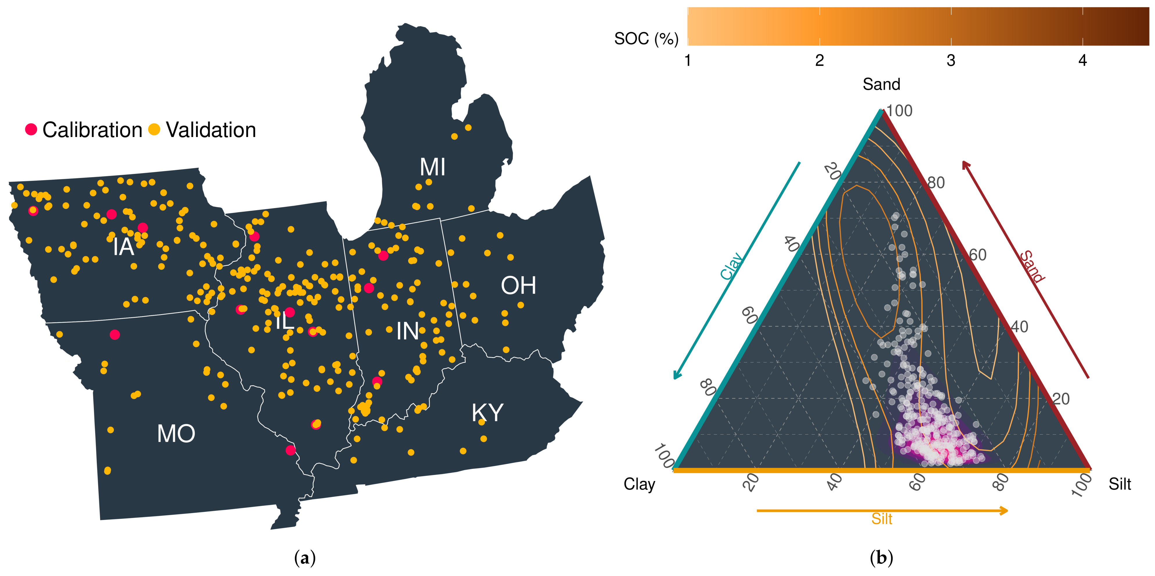
The study area for this modeling experiment extends over the Midwest region of the U.S., including sites in Iowa, Illinois, Missouri, Indiana, Michigan, Ohio, and Kentucky. The region was chosen because of its relative importance in global and domestic maize production [30]. Across the study area, maize was planted on an average of 16.5 ± 0.2 million ha from 2014–2019 [31]. To perform APSIM simulations at a series of randomly selected locations, site-level information was acquired from the publicly available maize yield dataset maintained by Beck’s Hybrids (https://www.beckshybrids.com/Research/Yield-Data, accessed on 30 November 2021). The dataset included information on management operations (i.e., planting date, harvesting date, plant population, row spacing, and previous crop planted for residue type), soil, and weather for 332 locations from 2014 to 2019 (Figure 2a). Information on soil texture and soil organic carbon (SOC) across the study sites is presented in Figure 2b. Each location consisted of a field varying in size from 0.3–0.5 km. Multiple hybrids were grown simultaneously, and as a consequence of the within hybrid variability, average maize yield was used as representative of the location as elaborated in [32].

Figure 2.
(a) Geographical location and (b) distribution of basic soil properties of calibration and validation sites. SOC: Soil Organic Carbon.
2.3. Data Collection
2.3.1. Weather and Soil
All the simulations conducted in this study, including those used in the sensitivity analysis, emulator development, and final yield validation, were performed by leveraging the uncertainty propagation workflow detailed in [12]. A Monte-Carlo sampling approach was used to propagate uncertainties in soil properties, meteorological variables, and unknown management practices. To propagate uncertainty in soil properties, 25 different representations (ensembles) of the soil profile were sampled for each site using the mean and uncertainty values retrieved from the SoilGrids dataset [33]. 10 ensemble members from the ERA5 reanalysis data product [34], which provides weather information at a 0.25 degree spatial resolution, were employed to propagate uncertainty in meteorological forcing.
2.3.2. LAI and NDVI Retrieval and Data Processing
Sentinel-2 and Landsat-8 were used in this study to provide observations of Leaf Area Index (LAI) and NDVI, respectively, for the calibration sites. These variables were selected mainly because they have been shown to be strong predictors of crop yield [35]. Sentinel-2 provides measurements of surface reflectance with 10 m–60 m spatial resolution depending on the spectral band with 5 days revisit time, while Landsat-8 images have 30m spatial resolution with 16 days revisit time. The forward model used for the LAI retrieval is a canopy radiative transfer model PROSAIL (PROSPECT + SAIL) [36], which takes inputs of bio-physical parameters, defining the state of canopy structure, leaf structure and leaf pigments (Table A2), and soil background, generating canopy level reflectance spanning 400–2500 nm. In order to cover a wide variety of soil conditions for different land surfaces, the soil reflectance model in the original PROSAIL model is replaced with one derived from wider samples. A spectral library of more than 6000 soil samples from public available soil databases (Table A1) is used to derive a soil model Equation (1) based on principle components analysis (PCA):
where is the simulated soil reflectance, is the mean value of soil reflectance from the spectral library, is the ith component of the PCA analysis and is the weight for the ith component. To simulate different soil spectra with the proposed soil model, weights for each component are randomly sampled within the bounds of PCs’ weights from the original soil spectral library. Then, the forward model PROSAIL M is used to simulate the surface reflectance R with the inputs of and can be expressed as:
Using inverse emulators Neural Networks (NNs) W, the mapping from the top of canopy (TOC) reflectance r to canopy state parameters is described as:
Bounds for , shown in Table A2, are used to generate samples from the PROSAIL model with uniform distributions.
The practical processes are described as:
- Randomly sampled 400,000 combinations of PROSAIL input parameters with bounds shown in Table A2 and weights for the soil model.
- Using PROSAIL to compute top of canopy reflectance with the randomly sampled inputs and the simulated soil background.
- The simulated reflectance is convolved with the Sentinel-2 relative spectral response functions to simulate surface reflectance at different bands (addB02, B03, B04, B05, B06, B07, B08, B8A, B11, B12).
- Train NN for LAI by using the simulated reflectance over Sentinel-2 bands as inputs.
- The trained NN is then used to map from satellite surface reflectance to LAI.
After retrieving LAI and calculating NDVI, a double logistic model was fit to each time series to remove noisy observations. NDVI values of below 0.5 were not used for further model optimization, because the surface reflectance signal is dominated by background soil reflectance compared to canopy reflectance early in the growing season resulting in often unreliable retrieval of plant traits.
2.3.3. Crop Growth Model
The APSIM classic (version 7.10) was employed and constrained in this study. As one of the most widely used crop modeling platforms, APSIM uses meteorological forcing and detailed soil information to simulate soil water, soil carbon (C), and soil nitrogen (N) dynamics at a daily time step and to generate predictions of crop growth and development. APSIM has been extensively tested and validated across the U.S. Midwest and has been used for exploring new management practices [22], as well as crop yield prediction at both the regional [12,37] and farm scale [10,38].
The Maize module in APSIM simulates the growth and development of a maize crop in response to climate, soil water, and soil N [7,39]. Leaf area development in the maize module is estimated based on total leaf number and leaf area [40]. Furthermore, the maize module allows for thermal time accumulation between 0 to 10 C, providing a more accurate simulation of maize phenology in cool environments [41]. Estimating daily leaf area development in the maize module begins by calculating the potential increase in leaf area from new leaves which is driven by thermal time and leaf size [42]. The potential leaf area is then limited by the biomass accumulation (carbon supply) and the number of expanded leaves [40]. Therefore, the accuracy of LAI predictions in the Maize module is dependent on both the accurate simulation of phenology as well as the crop-specific parameters controlling leaf size, leaf appearance rate, and biomass partitioning.
To estimate canopy reflectance, this study coupled APSIM with PROSAIL (version. 5B) (a Radiative Transfer Model) through the C# manager module. The PROSAIL model integrates the PROSPECT leaf optical properties model and the SAIL canopy bidirectional reflectance model to effectively simulate the crop canopy reflectance as a function of leaf biochemical traits, canopy architecture, soil background, and sensor geometry [36]. At the end of each day and for each ensemble member, C# manager passes a series of soil and plant state variables to the PROSAIL model to compute spectral reflectance. The reflectance profile simulated by the PROSAIL model was then used to estimate APSIM NDVI for each site, which was then compared to site-level Landsat-8 NDVI estimates. Site-level LAI estimates from Sentinel-2 were directly compared with model LAI predictions.
This study closely followed the coupling procedure detailed in [43]. In addition to LAI, which was directly passed to the PROSAIL model from APSIM, the remaining PROSAIL inputs were estimated as follows and the detailed definition of each parameter with its associated possible range and unit is provided in Table A2:
where SLA is the specific leaf area per dry weight (), is soil wetness/dryness factor, SWC is the actual soil water (), SAT is the soil water at saturation (), DM is the dry matter () and NP is the percentage of green leaf nitrogen (%). The other 9 parameters within the PROSAIL model were either directly extracted from the EO images or set using the same default values as given in Table 2 of [43]. These parameters are mainly related to the viewing geometry of sensor, crop type, and day of the year. The viewing parameters (hotspot, solar zenith angle, observer solar angle, azimuth) were extracted directly from the image properties, while other biophysical parameters (Cbrown, Cw, leaf Angle) were set according to the values provided by [43,44,45].
2.4. Model and Parameter Selection
A global sensitivity analysis (GSA) was performed prior to model calibration on 14 Maize module parameters across 13 training sites. Parameters were selected which control, to some extent, the estimation of LAI in the model. GSA is usually performed to reduce the dimensionality of crop model calibration techniques by identifying the most influential model parameters for a particular model output. In this study, the candidate parameters influencing LAI were chosen based on [40], which laid the foundation for LAI estimation in the Maize module. A time-variant, Analysis of variance (ANOVA) based GSA was employed to identify parameters that explained the largest variation in LAI during the growing season across the 13 sites.
Prior to GSA, a power analysis was conducted to determine the minimum sample size required for detecting an effect size as small as 0.01 with . Our power analysis showed that, with 2500 simulations, our ANOVA-based GSA would be able to detect effects as small as 0.01 with more than 95 % power () for 4 model parameters.
For the GSA, a total of 2500 simulations were executed for each site using random samples taken from the candidate parameter space. Then, a linear model was fit to predict simulated LAI as a function of the sampled parameters at 30 different time steps during the growing season in 2018 and 2019. The contribution of each parameter was calculated as the proportion of variability in LAI estimates that it explained at each time step. The total sensitivity of each parameter was estimated as the Sums of Square (SSQ) ratio following [18,22]
2.5. Emulator Development
Given that most optimization techniques require frequent evaluation of the process model, most prior stochastic Bayesian optimization studies have focused on simple crop models, as applying such techniques with slow process-based models would impose a computational burden. To overcome this limitation, this study leveraged more computationally efficient surrogate models (emulators) instead of the full APSIM model when performing optimization. Emulators are statistical models that are faster to run and can replicate the behaviour of the full model within a constrained parameter space [46].
To develop the the site-level emulators for optimization, we used a Latin hyper cube sampling method to generate 250 samples for the most sensitive parameters found in the GSA under broad, non-informative priors. Then, for each sampled point in the parameter space, the model was run with 50 ensembles (accounting for the uncertainty in soil and weather data) at each site to generate LAI estimates. Average estimates of LAI were then computed for each sampling point at each site and used as the response variable in the emulator development stage. Emulators were developed using Generalized Additive Models (GAM) as follows:
where t represents time and Pi represents the ith most sensitive parameter. The emulators were fitted independently at each site and predict an LAI time series at days with available observations as a function of the most sensitive parameters.
2.6. Optimization Schemes
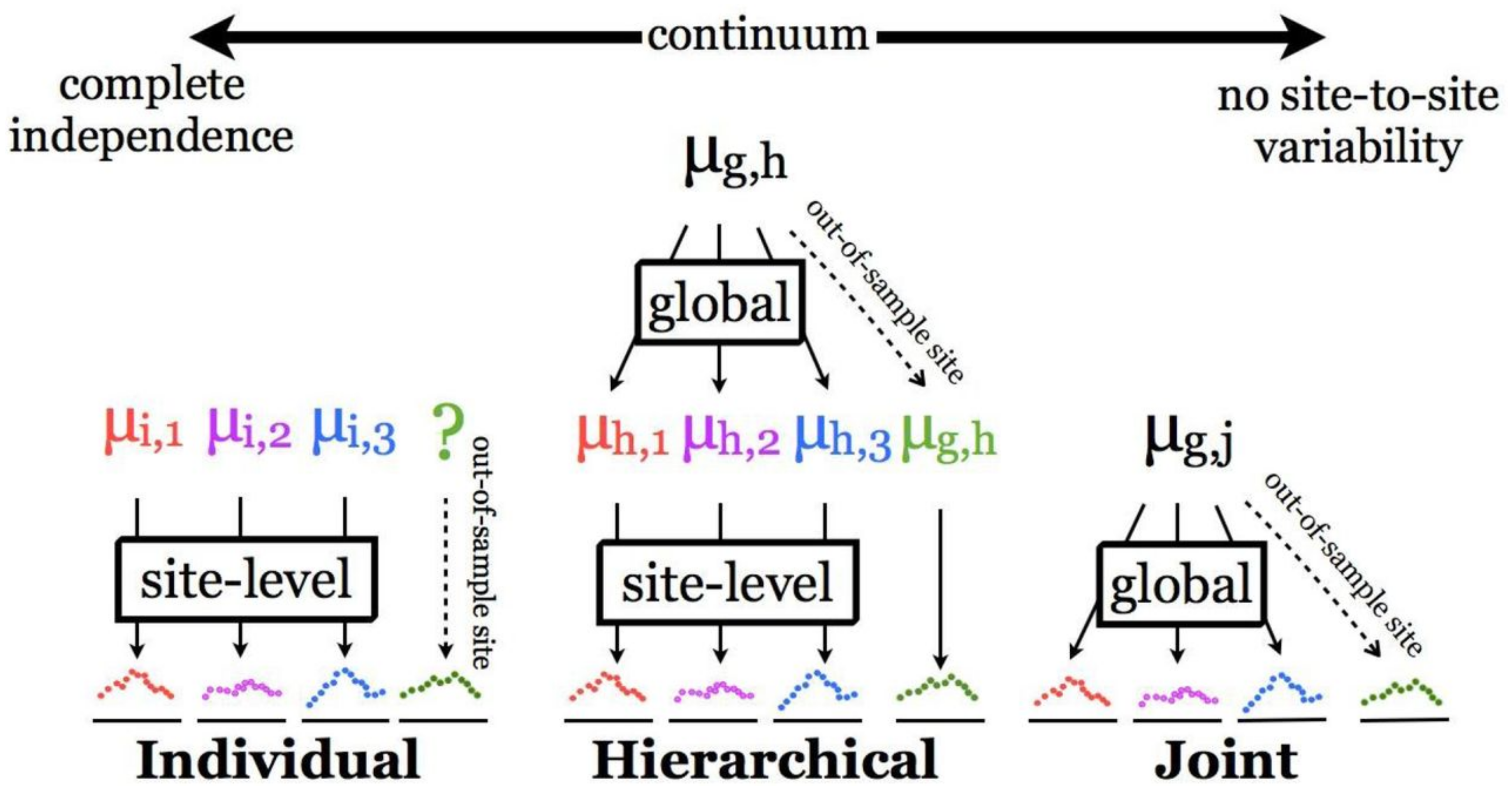
This study explores three different Bayesian optimization schemes with each scheme varying in the degree to which observations are shared across different sites. The site-level optimization scheme assumes full independence between observations collected at different sites, while the global (joint) optimization scheme shares all observations across all sites and attempts to find a set of optimum parameters that maximizes the likelihood of monitoring observations across all sites simultaneously (Figure 3). These two optimization schemes are widely used for constraining process-based ecological and crop growth models [22]. However, it has been demonstrated that the full independence assumption in site-level optimization limits the extent to which results can be up-scaled or applied to new sites [17]. Prediction at new sites will be unreliable and overconfident. In addition, neither scheme offers a solution for quantifying or propagating spatiotemporal variability in model parameters [17].

Figure 3.
Graphical representation of different optimization schemes explored in this study to constrain model parameters, as adopted from [17].
Alternatively, a hierarchical optimization scheme (HPDA; Figure 3) allows for sharing information across sites and attempts to capture site-to-site variability in model parameters by estimating a series of site effects. The unexplained variability captured in site effects can help to reveal missing processes in the process model and to account for systematic biases in model inputs and/or parameters. This scheme estimates a global mean, as well as site-level means which vary around the global mean by an estimated random site effect. By estimating site effect variance in HPDA, we quantify the portion of total variability in model parameters which can be attributed to variability between sites.
To compare the site-to-site variability among parameters, the standard deviation estimated for site effects was used with the HPDA joint mean estimate to calculate a unit-less coefficient of variation. All statistical models for the optimization schemes (Table 1) were fit using the NIMBLE package in R [47]. Consistent uniform priors were selected for all parameters across all optimization schemes to ensure objective estimation of parameter posteriors.

Table 1.
Model definition for different optimization schemes explored in this study. Across all schemes, represents the vector of model parameters, k represents observations or parameters for site k, Y represents LAI and NDVI observations, and f represents the emulator.
We assessed the information contribution of NDVI for constraining model parameters by performing two HPDA optimizations: one with both data constraints and one with only LAI as a data constraint. The shrinkage in prediction uncertainty associated with LAI and NDVI constraints was then estimated as the ratio of the coefficients of variation for the two HPDA optimizations (i.e., both:LAI only). When this ratio is less than one, it represents a larger shrinkage of prediction uncertainty with both data constraints, while a value greater than one indicates LAI alone led to greater shrinkage.
The model predictions of yield after optimization was compared against observed yield for both within and out-of-sample predictions using the following statistics:
where is the observed yield and is the corresponding simulated yield. In addition, is and is with representing the average observed yield [48].
3. Results
3.1. Sensitivity Analysis and Emulator Performance
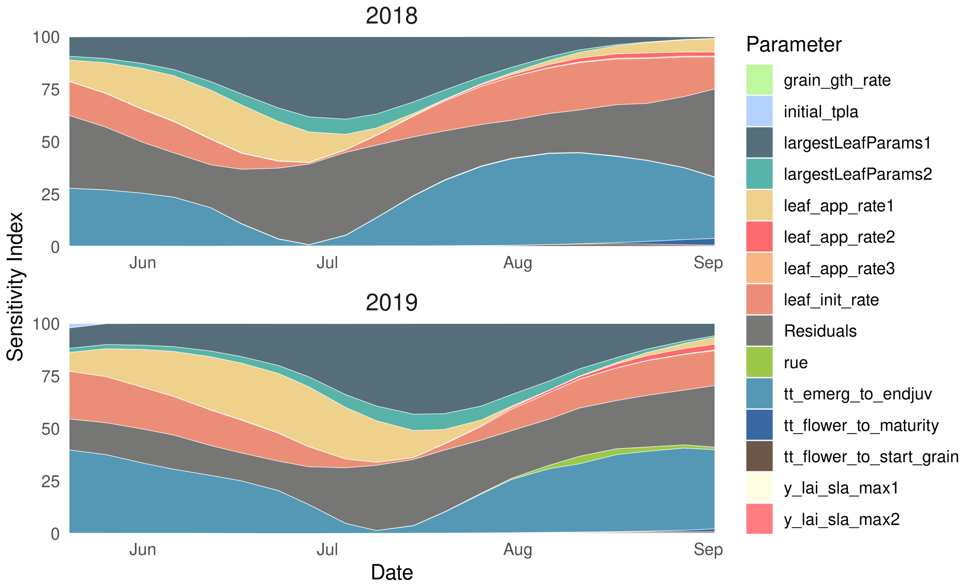
The 14 parameters included in the GSA were those within APSIM that control leaf appearance (e.g., leaf_init_rate, leaf_app_rate1), growth (e.g., largestLeafParams1), and development (e.g., tt_emergence_to_endjuv). The time-varying GSA demonstrated the dynamic contribution of all 14 parameters in explaining LAI variation across all sites for 2018 and 2019 (Figure 4). Similar patterns were found across both years and all sites, where the 14 included parameters accounted for ≈ 80% of the variation in LAI between early June until early September. However, the predictive power of the selected parameters diminished from early September until early November, at which point these parameters explained only ≈ 10% of the variability. After this initial set of parameters loses its predictive power in early September, the residuals—which describe the contribution of all other factors to LAI variability—keep increasing till the end of October. We speculate that parameters controlling leaf senescence would make up much of the residual contribution towards the end of growing season.

Figure 4.
Average sensitivity index for maize leaf area index (LAI) corresponding to 14 model parameters in APSIM across all sites for years 2018 and 2019.
Of the 14 parameters included in the GSA, the largestLeafParams1 and the thermal time from emergence to the end of the juvenile stage (tt_emergence_to_endjuv) were the most influential parameters, together explaining ≈40% of the LAI variability at their peak contribution. In addition, leaf_init_rate and leaf_app_rate1 together explained a maximum ≈20–25% of the LAI variability. Therefore, we selected these four parameters for emulator development and optimization in this study as they are the most influential parameters for LAI estimation in the APSIM Maize module. Following [40], APSIM uses a nonlinear continuous equation to estimate the total leaf area as a function of the leaf number (determined by growing degree days and leaf appearance rate) and the area of the largest leaf, where maximum leaf area is limited to 1000 cm per plant. Looking at our most influential parameters, largestLeafParams1 helps determine the largest potential leaf area, while leaf_init_rate and leaf_app_rate1 helps to control the total leaf number. Further constraint of the largestLeafParams1 parameter was especially warranted as the original model proposed by [40] was developed with a relatively small sample size (n = 18).
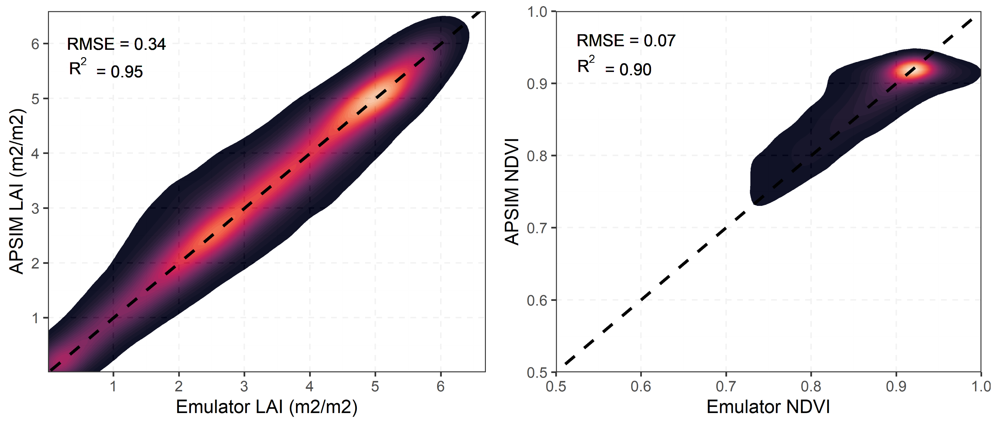
To assess the predictive power of the emulators, APSIM estimates of NDVI and LAI were compared against emulator estimates (Figure 5). Both the LAI and NDVI emulators showed strong predictive capacity with of 0.95 for LAI and 0.90 for NDVI, demonstrating their ability to replicate APSIM behavior given the most influential parameters found in the GSA (Figure 5). We speculate the variability around the 1:1 line for both LAI and NDVI predictions stems from the uncertainty propagated in APSIM simulations (Figure 5). This uncertainty can be associated with soil properties, meteorological forcing, and management practices.

Figure 5.
Density plots comparing emulator and APSIM estimates of LAI and NDVI across calibration sites. The lighter colors represent higher density of points and darker color represent lower density of points.
3.2. Within Sample Prediction
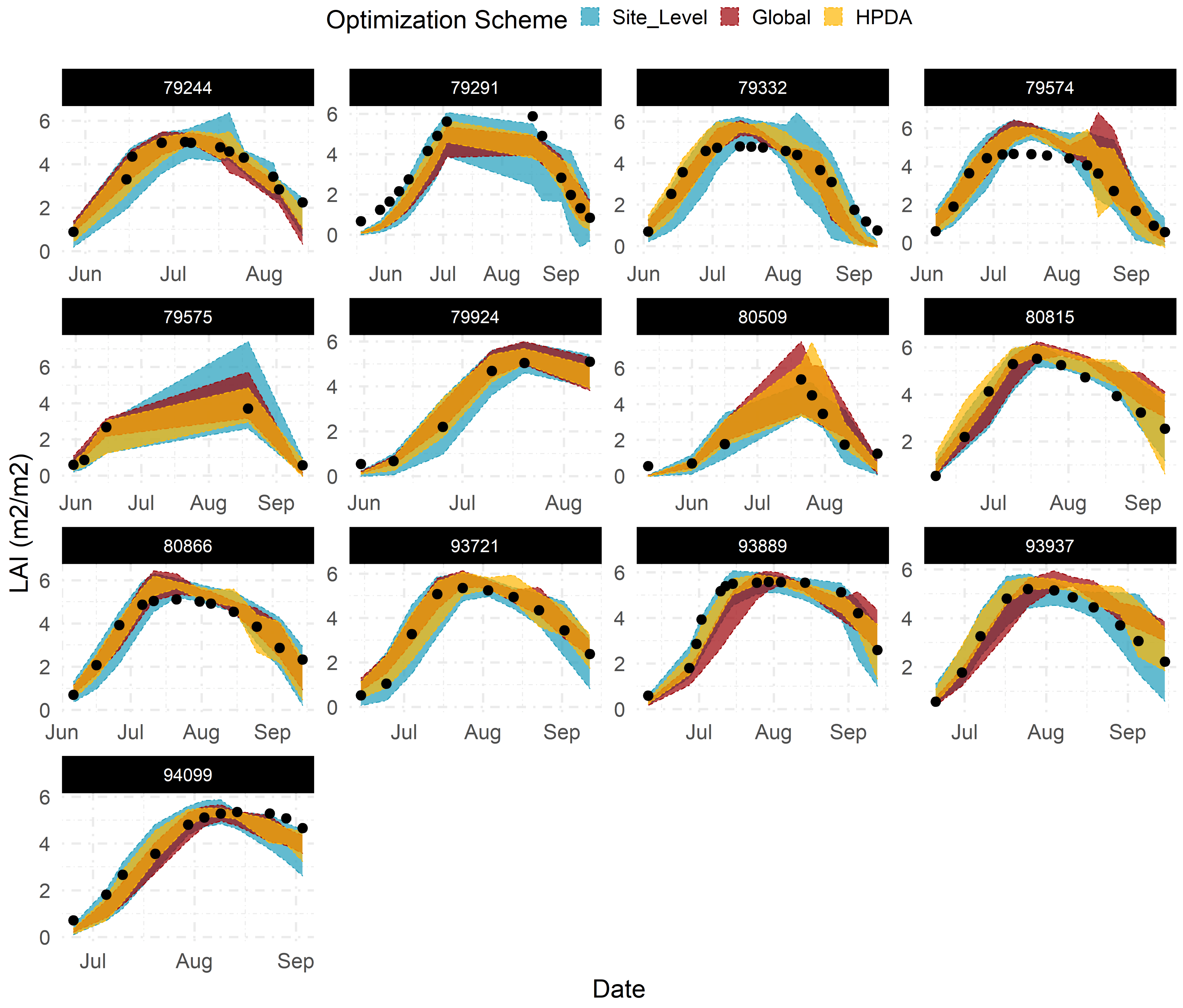
Emulators showed sufficient flexibility in replicating the dynamic behavior of LAI and NDVI throughout the growing season across all sites when given the most sensitive parameters (Figure 6). Across all sites, site-level optimization showed the largest predictive uncertainty around LAI and NDVI estimates, whereas global optimization demonstrated the most constrained predictions. This behaviour was expected as it closely relates to how each statistical model (Table 1) shares information across sites and, consequently, the number of observations available to each model for “learning” LAI and NDVI patterns.

Figure 6.
95% confidence interval for emulator predicted LAI using optimized parameters corresponding to each optimization scheme across all calibration sites.Title for each subplot corresponds to the site ID in Beck’s dataset.
With site-level optimization, only observations available at each site are used to estimate the model parameters. As a result, we found greater constraint of LAI and NDVI predictions for sites with a higher number of observations (e.g., site 80866, 94099 and 93889) compared to sites with larger data gaps (e.g., site 79575) (Figure 6). With global optimization, all observations across all sites are used simultaneously for estimating model parameters. Global optimization ignores the structure in the data and provides mean parameter estimates that maximize the likelihood of all observations when using all site emulators simultaneously. This increases the total number of observations available for estimating model parameters compared to the site-level approach. HPDA, on the other hand, attempts to capture the site-to-site variability by adding random effects for each site, while still leveraging all available observations. Site effects in HPDA account for another layer of uncertainty around the global mean estimate for each parameter and naturally resulting in more uncertain LAI and NDVI predictions compared to global optimization (Figure 6).
All optimization schemes showed similar d-index values in LAI prediction across all months and sites (Table 2), though global optimization showed a marginally lower d-index, on average, when compared to the site-level and HPDA schemes. A similar pattern was found for RMSE such that the site-level and HPDA schemes showed lower RMSE than the global optimization. However, it was found that the site-level scheme largely underestimates LAI compared to the global and HPDA optimizations with Mean Error (ME) of −0.16 kg/ha compared to −0.08 and −0.07 kg/ha for global and HPDA optimization schemes, respectively.

Table 2.
Performance of different optimization schemes across different months for LAI.
To assess the contribution of NDVI observations in shrinking LAI prediction uncertainty within the HPDA scheme, the prediction coefficient of variation (CV) under both data constraints was compared with that under only LAI constraint using a ratio. Shrinkage in model uncertainty with added NDVI constraint was dependent on site (or possibly data quality at each site) and month of the year. The largest reduction in LAI uncertainty after adding NDVI was found in May, August, and September, and the largest reduction in NDVI uncertainty was found in May and August (Figure A3).
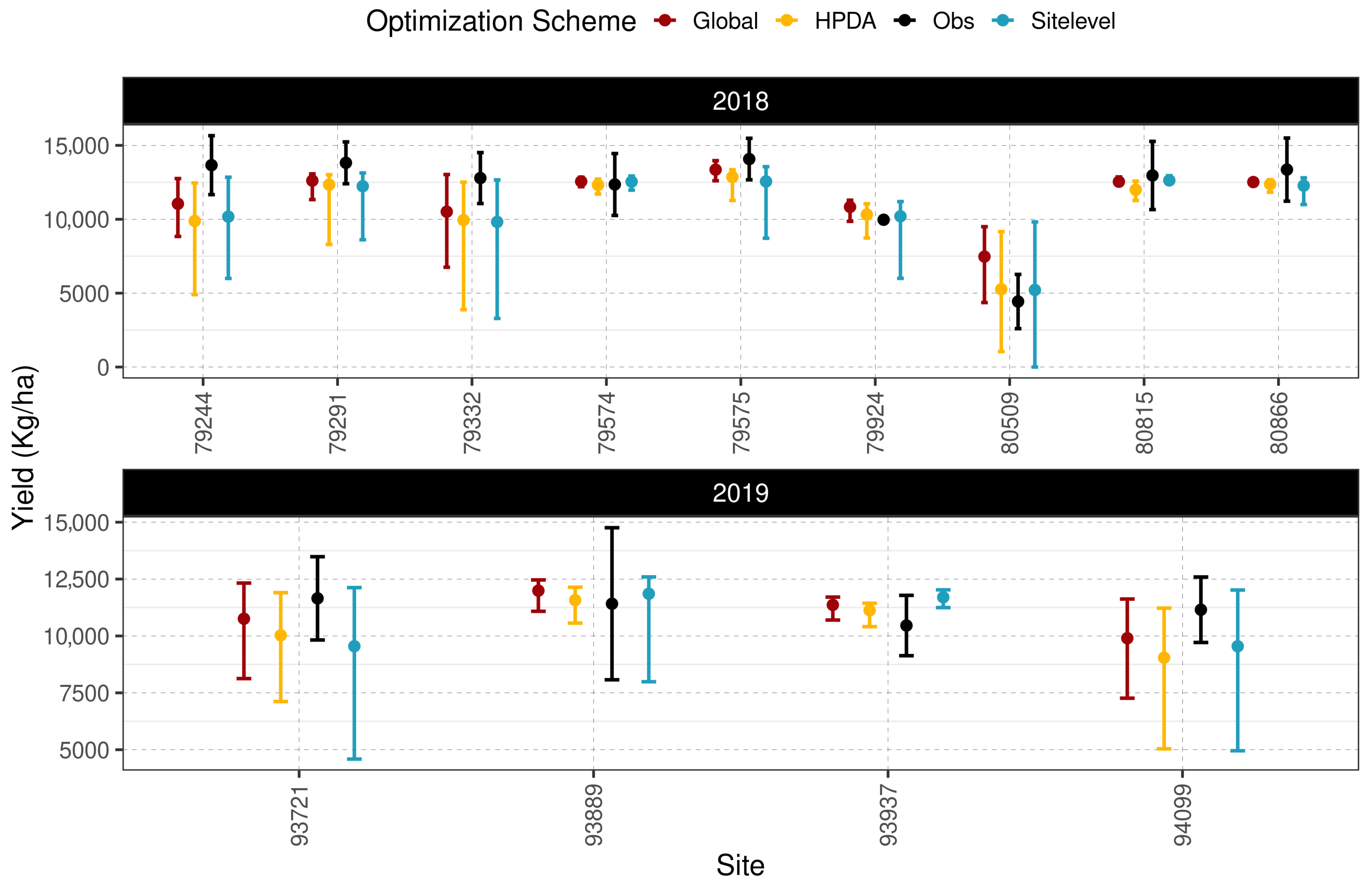
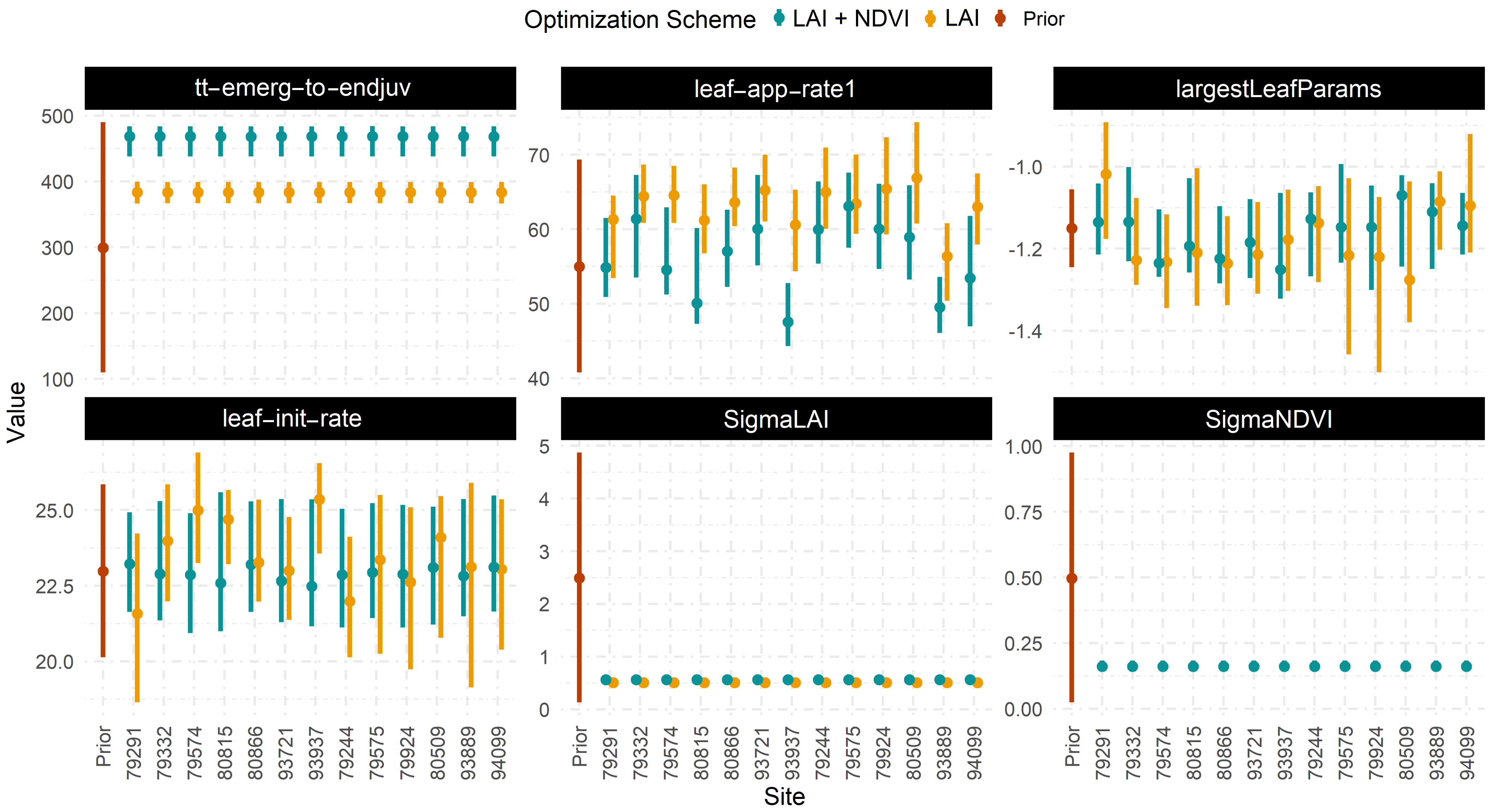
Including NDVI in the HPDA optimization resulted in more constrained estimates of largestleafParam1 and shifted the mean site-level estimates of tt_emergence_to_endjuv up (Figure A5). In addition, both scenarios resulted in a similar mean suggesting a minimal contribution of NDVI in closing the gap between model estimates and observations. All optimization schemes performed similarly for within-sample yield prediction, with RMSE values ranging from 1423 () for HPDA to 1494 () for site-level optimization (Figure 7). HPDA showed the highest d-index (0.9), whereas global optimization showed the lowest d-index of 0.85. Among all optimization schemes, the global scheme showed the lowest mean error (ME) of −282 (), whereas HPDA showed the largest ME of −780 (). Furthermore, as expected global optimization showed the lowest median CV for both years in within sample yield prediction followed by HPDA and then the site-level scheme (Figure A1).

Figure 7.
95% Confidence interval for within sample yield comparison between different optimization schemes.
3.3. Comparing Posterior Distributions
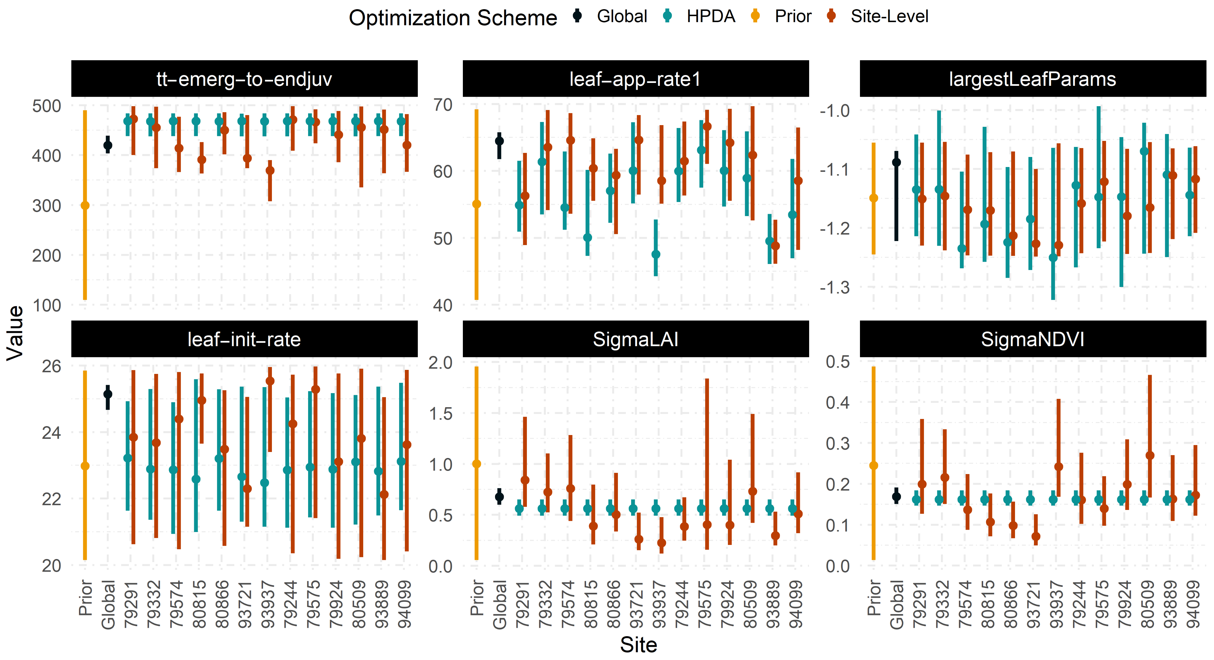
Though we set identical priors for each parameter across all optimization schemes (Figure 8), the most constrained posterior densities were found for tt_emergence_to_endjuv and leaf_app_rate1 across all sites and optimization schemes. Global optimization offered the most constrained set of posterior distributions for all parameters, whereas site-level optimization estimated the least constrained set of posteriors and exhibited variable constraint across different sites.

Figure 8.
95% Confidence interval for various crop model parameters across different optimization schemes and sites.
Since the site-level and HPDA schemes are more reliant on the quality and quantity of observations available at a given site, the degree to which they were able to constrain model parameters varied significantly with site. In site-level optimization, the largest site-to-site variability was found for tt_emergence_to_endjuv ( = 9.5 %), while the lowest variability was estimated for largestleafParam1 ( = 5%). Similarly, the largest site-to-site variability within the HPDA was found for leaf appearance rate with an average CV of 9% while tt_emergence_to_endjuv showed the least variability with a CV of 2 %. Greater parameter constraint with the global optimization scheme (Figure 8) resulted in narrower confidence intervals around LAI and NDVI predictions (Figure 6). Alternatively, prediction intervals depend on in sites with greater mean estimates of and often showed larger prediction intervals.
In addition, no statistically significant relationship was found between variability in model parameters and the quality of fit ( and ). Sites with fewer observations had substantially larger values of relative to those estimated with the global and HPDA schemes. We found a statistically significant and lower value of for site 93937 which, interestingly, demonstrated a trade-off with a higher value of .
3.4. Out-of-Sample Prediction
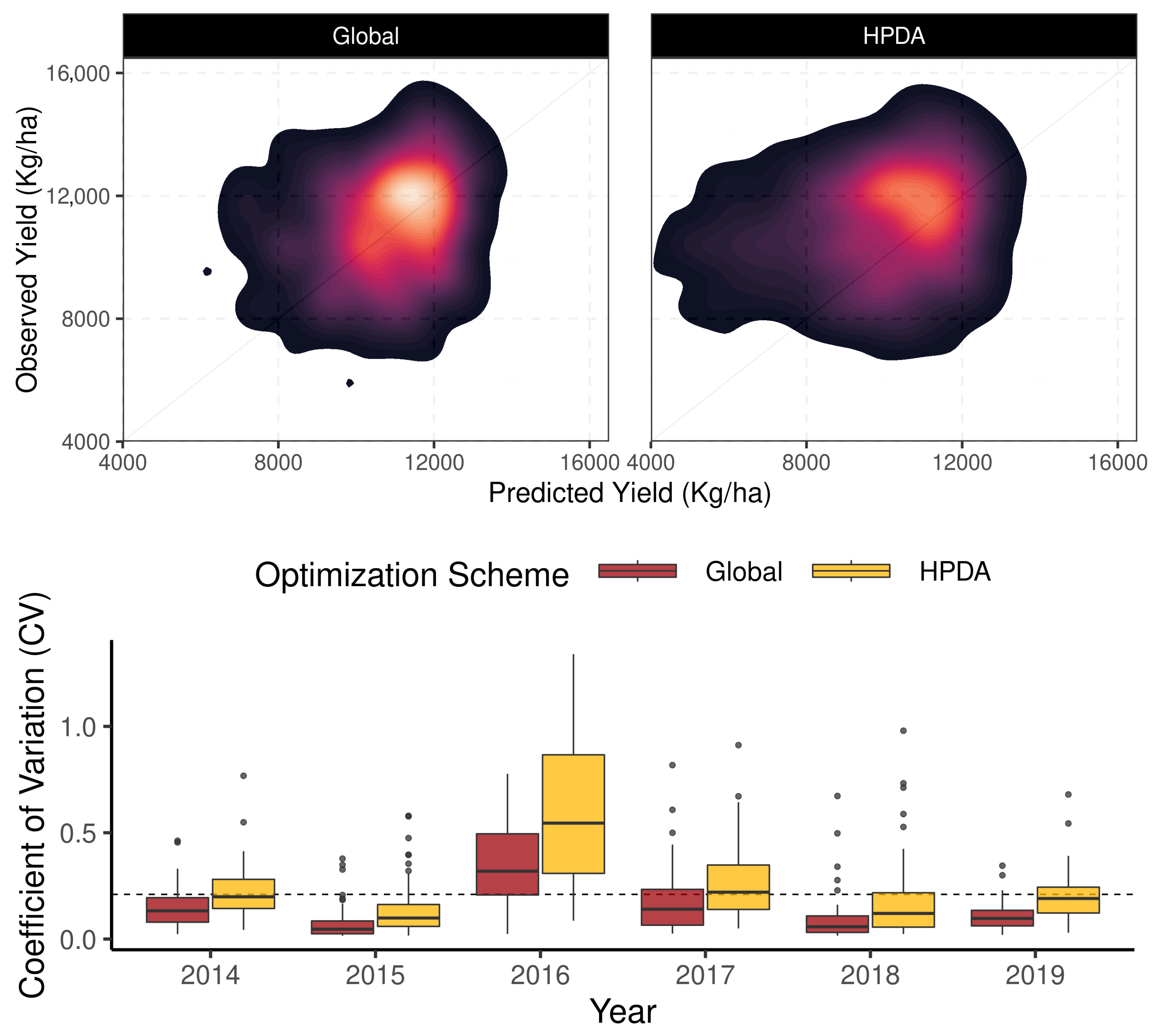
The evaluation of the optimization schemes for predicting crop yield was carried out at 325 sites independent of those used for optimization (Figure 9). Since site-level optimizations cannot be generalized to new sites, this optimization scheme was dropped from evaluation. The HPDA and global optimization schemes reported similar d-index values (0.55 for Global and 0.51 for HPDA ) for evaluation when averaged across all sites and years (Table 3). The global optimization, however, reported a lower RMSE for crop yield (1768 kg ha) than HPDA (2296 kg ha) and, similarly, the ME for global optimization and HPDA was estimated to be around −66 kg ha and −939 kg ha, respectively when averaged across all sites and years. The ME values from year to year showed that the HPDA optimization systematically underpredicted crop yield at the evaluation sites.

Figure 9.
Density plots comparing yield estimates for out of sample sites (top), and yield variability (bottom) for global and HPDA optimization schemes.

Table 3.
Comparing model performance in simulating crop yield on out of sample sites for outside (2014–2017) and within the (2018–2019) the spatiotemporal extent of training dataset.
To assess whether there was a spatial pattern in the underestimation of crop yield, we divided the sites into two different categories: ‘within’ the spatial extent of calibration sites and ‘beyond’ the spatial extent of calibration sites. Following this approach, 242 sites were classified as ’within’ and 90 sites were classified as ’beyond’ of the 332 sites evaluated (Figure A4). When HPDA and global optimization schemes were compared only within the temporal and spatial extent of the training sites (90 sites), both approaches showed robust (less variable) and similar performance in maize yield prediction with RMSE values ranging from 1.6–1.8 Mg/ha for global and HPDA predictions, respectively (Table 3). When HPDA and global optimization predictions were compared for sites outside the spatiotemporal extent of the training dataset (242 sites), global optimization performed substantially better than HPDA with average RMSE of 1838 Mg/ha for global versus 2500 Mg/ha for HPDA (Table 3). For these ’beyond’ predictions, lower precision in yield prediction was found for HPDA on average whereas global optimization consistently showed lower uncertainty compared to HPDA. This is mainly due to the fact that the HPDA global mean estimates for parameters is inherently more uncertain.
This study solely relied on EOs to calibrate and validate the APSIM model across an unprecedented number of sites with large spatiotemporal variability, but the results of model validation still showed similar performance to prior site-level APSIM calibrations with field observations. For instance, ref. [49] calibrated APSIM using 56 site-years of data from 8 field studies across six states in US Midwest for maize-maize rotation. They reported grain yield RMSE at the site-level (not summarized) with values ranging from 1.35–2.97 Mg/ha. Ref. [23] calibrated APSIM using a time-dependent parameter estimation framework to better capture maize yield variability due to changes in cultivar and management. They parameterized 9 parameters for maize cultivar across the US Corn-Belt using three different calibration methods and compared predictions to 9 machine learning models. Their calibrated APSIM model showed RMSE values between 0.865–1.459 Mg/ha over the 5 sites for the time period between 1985–2018. Ref. [50] calibrated APSIM for seven experimental sites in the Midwest (including sites in southern Minnesota, Iowa, Indiana, and Ohio). After calibration, their model achieved an RMSE of 1.27 Mg/ha for maize yields. Lastly, ref. [25] compared two different formal (DREAM) and informal (GLUE) Bayesian optimization approaches in calibrating an APSIM maize model and reported RMSE ranging from 0.274–2.1 Mg/ha across 6 maize cultivar on the north China plain.
4. Discussion
Although direct measurements are not available for all optimized parameters, a recent study by [51], explored the variability of leaf appearance rate across 98 sites for maize in the U.S. Midwest. Their results showed that the average first phase phyllochron for modern maize hybrids in the U.S. Midwest is 57.9 ± 7.5 (C-day). This aligns with the results of this study, such that the mean estimates of this parameter was 64, 60 and 56 (C-day) for the global, site-level, and HPDA schemes, respectively. In another study with manual calibration, ref. [27] found that leaf appearance occurs at a rate of 57 (C-day), a rate that is significantly faster than APSIM maize’s default rate of 65 (C-day) in the U.S. Corn Belt.
Similar to [17], who did not find any improvement in model accuracy using HPDA over global optimization scheme on “out-of-sample” sites, we did not find any improvement in maize yield prediction using HPDA. However, ref. [17] suggested that the difference in performance between HPDA and global optimization will increase in favor of HPDA as the number of sites/parameters increases. In contrast to completely generic (global) or completely site-specific (site-level) model parameters, HPDA offers an alternative solution that allows under-sampled sites to borrow strength from sites with more data to achieve better constraint in model predictions [52,53]. HPDA has the advantage of having a formal distinction between prediction at known calibration sites and “out-of-sample” sites [17]. When predictions are made for “within-sample” sites, site-level parameters (, Table 1) can be used to make predictions, whereas the global mean () estimated through HPDA is used to make predictions on “out-of-sample” sites. Furthermore, when designing HPDA optimization schemes, extra attention needs to be paid in deciding which parameters should be random. By attempting to capture site-to-site variability, the total number of parameters in our hierarchical model increases, which could be limiting in cases with low sample sizes. However, this is less of a concern for EOs given their extensive spatiotemporal coverage and larger sample size compared to field experiments. Similar to [23] which accounted only for the effect of year in APSIM model parameters, future works on HPDA also may need to explore the impact of including a year effect in addition to the site effect to estimate the full spatiotemporal variability in APSIM maize parameters.
Site-level model calibration showed variable performance in constraining LAI and yield estimates, with performance operating as a function of data density across within-sample sites. This points to the inherently limited nature of this calibration scheme for application to broad regions. Moreover, this limitation in site-level calibration is even more pronounced due to the “perfect model” assumption behind all calibration procedures. The “perfect model” assumption ignores any structural error in process-based crop models, assuming discrepancies between model estimates and data originate solely from non-optimum parameters. Calibration attempts to correct for these discrepancies in the model by adjusting the parameter values so that the model performs well within the domain of the training dataset. However, due to biased parameter estimates which often differ from the “true” parameter values, the final parameterized model often underperforms in out-of-sample sites [54].
Ref. [54] suggested it is often impractical to fit multiple data streams simultaneously using complex computer simulation models due to internal constraints, such as mass balance and structural error. They argued that calibration schemes tend to find an optimum set of parameter values that corrects for error in the more data-rich output at the cost of larger errors or overly narrow confidence intervals in data-poor streams. In this study, though an unbalanced dataset of LAI and NDVI was used, APSIM performed reasonably well in simulating both outputs and, overall, no trade-off was found between NDVI and LAI predictions (e.g., Site 79924).
No significant correlation was found between maximum a posteriori of optimized parameters and different soil or weather variables across all training sites suggesting that the estimated site effect is potentially also reflecting a confounding G X E effect and not just an environmental (’E’) effect. However, in order to untangle this confounding G x E interaction, more replications are needed for the cultivars used in the training sites. In a similar study, ref. [17] calibrated the the Simplified Photosynthesis and Evapotranspiration (SIPNET) model through HPDA across 12 temperate deciduous Ameriflux sites. They identified a missing temperature response in respiration and photosynthesis and associated it with a lack of thermal acclimation and adaptation in the model. The missing temperature response was found due to large site-site variability (’E’ effect) found in parameters related to these processes.
For within-sample model application, the global optimization approach offered the most robust (least variability) parameter estimates and provided the most well-constrained LAI and yield predictions. This shows the potential for global optimization in low sample size prediction problems. Global optimization also performed substantially better than HPDA in “out-of-sample” sites, especially when sites fell outside of the spatiotemporal extent of the training data (Table 3).
Ref. [55] states that describing the state of knowledge for complex ecological systems clearly and accurately is only possible when one has accounted for all sources of uncertainty. These sources include uncertainty in model parameters, initial and boundary conditions, and agricultural practices [12], similar to those propagated in this study. Bayesian optimization techniques offer a systematic approach for accounting for these uncertainties [56,57] and are often preferred over numerical methods for calibrating process-based crop models because (1) when new data becomes available, posterior densities from previous studies can be used as an informed prior to rapidly incorporate new information and (2) Bayesian techniques allow for incorporating error in observational data, which, given the noisy nature of EOs, can be essential to account for true uncertainty in model parameters [21].
The larger sample size and multi-faceted observational data provided by EOs can potentially reduce the risk of equifinality in model calibration by constraining multiple parameters/state variables in models simultaneously. Furthermore, recent advancements in mapping and monitoring crop phenology [58] through EOs could be leveraged in addition to retrieving biophysical variables, like LAI, to further increase the number of data constraints and adjust crop phenology accordingly. Process-based crop models are often calibrated under no-stress conditions which is impractical given the nature of EOs. However, as a future direction, we will work towards including additional parameters that control water/N stress within the optimization problem. This could be particularly important as [51] reported that water and nitrogen stress may delay phenology and leaf appearance in maize across the U.S. Midwest.
Our proposed framework is novel among previous model calibration efforts in that it (1) incorporates and leverages site-to-site variability in optimization, (2) employs EOs to constrain model parameters, (3) accounts for observation uncertainty and estimates parameter uncertainty, and (4) follows a systematic calibration approach that could be updated as new data becomes available for new sites. This work demonstrated a proof-of-concept for direct application of EOs in constraining and improving yield prediction with the APSIM model. Future works should consider upscaling this framework from 13 calibration sites to potentially hundreds of sites with sufficient sample sizes on different crops/cultivars to fully explore the inherent spatiotemporal variability of APSIM model parameters. Furthermore, the effect of increase in the total number of data constraints and their spatial resolution on crop yield and optimized parameters needs to be further investigated.
5. Conclusions
This study demonstrated the use of EOs for calibrating parameters in complex process-based crop models through different optimization schemes that vary in the degree to which information is shared across sites. A time-varying global sensitive analysis performed on 13 sites helped identify the most influential parameters controlling maize LAI prediction in APSIM. GAMs were used as surrogate models to replicate the APSIM model behavior in simulating LAI and NDVI given the most influential parameters. These surrogate models were then used in three different calibration schemes including site-level, hierarchical, and global/join optimization. Overall, all optimization schemes showed similar performance in simulating crop yield for within-sample sites. However, global optimization demonstrated the most constrained LAI and yield estimates, while HPDA provided the most accurate yield estimates. For out-of-sample sites, global optimization provided both, the most accurate and most constrained yield estimates of the three optimizations.
Author Contributions
Conceptualization, H.D.; methodology, H.D.; software, H.D.; validation, H.D., T.R. and M.K.; formal analysis, H.D.; investigation, H.D., T.R. and M.K.; data curation, H.D.; writing, H.D., F.Y., M.K. and T.R.; review and editing, T.R., M.K., P.L. and J.L.G.-D.; visualization, H.D.; supervision, H.D.; project administration, H.D.; funding acquisition, H.D. All authors have read and agreed to the published version of the manuscript.
Funding
PL, JGD and FY would like to acknowledge support from the United Kingdom’s Natural Environment Research Council (NERC) National Centre for Earth Observation (NCEO) (projects NE/R000115/1 and NE/R016526/1), the Newton Prize (Newton Prize 2019 Chair’s Award, administered by BEIS), and STFC under project AMAZING - Advancing MAiZe INformation for Ghana (ST/V001388/1).
Data Availability Statement
The data presented in this study are available on request from the corresponding author.
Conflicts of Interest
The contact author has declared that neither they nor their co-authors have any competing interest.
Appendix A

Table A1.
List of spectral databases used in the study.
Table A1.
List of spectral databases used in the study.
| Library | Type | Reference |
|---|---|---|
| USGS v7 | Measurements | [59] |
| ICRAF-ISRIC | Measurements | [60] |
| Price | Soil model | [61] |
| Prosail | Soil model | [36] |

Table A2.
List of PROSAIL parameters used along with the APSIM-maize model in the study.
Table A2.
List of PROSAIL parameters used along with the APSIM-maize model in the study.
| Traits Type | Parameter | Symbol | Range | Unit |
|---|---|---|---|---|
| Canopy structure | leaf area index | 0–8 | m/m | |
| leaf angle distribution function | 0–90 | |||
| Leaf optical | chlorophyll a and b content | 0–120 | g/cm | |
| Carotenoid content | 0–25 | g/cm | ||
| Anthocyanin content | 0 | g/cm | ||
| leaf dry matter per leaf area | 0.002–0.01 | g/cm | ||
| leaf water content per leaf area | 0–0.04 | mg/cm | ||
| brown pigment content | 0–1 | - | ||
| mesophyll structure coefficient | N | 1–2.5 | - | |
| angles | solar zenith angle | sza | 0–80 | |
| viewing zenith angle | vza | 0–15 | ||
| relative azimuth angle | raa | 0–360 |

Table A3.
List of initial candidate parameters used in the global sensitivity analysis
Table A3.
List of initial candidate parameters used in the global sensitivity analysis
| Parameter | Upper Bound | Lower Bound |
|---|---|---|
| tt_flower_to_maturity | 1100 | 700 |
| tt_emerg_to_endjuv | 500 | 200 |
| tt_flower_to_start_grain | 400 | 100 |
| leaf_app_rate1 | 65 | 40 |
| leaf_app_rate2 | 50 | 20 |
| leaf_app_rate3 | 50 | 20 |
| largestLeafParams1 | −1 | −2 |
| largestLeafParams2 | 0.05 | 0.03 |
| y_lai_sla_max1 | 55,000 | 45,000 |
| y_lai_sla_max2 | 30,000 | 20,000 |
| leaf_init_rate | 30 | 15 |
| rue | 3 | 1.6 |
| grain_gth_rate | 11 | 8 |
| initial_tpla | 450 | 300 |

Figure A1.
Within sample yield variability comparison for different optimization schemes.
Figure A1.
Within sample yield variability comparison for different optimization schemes.
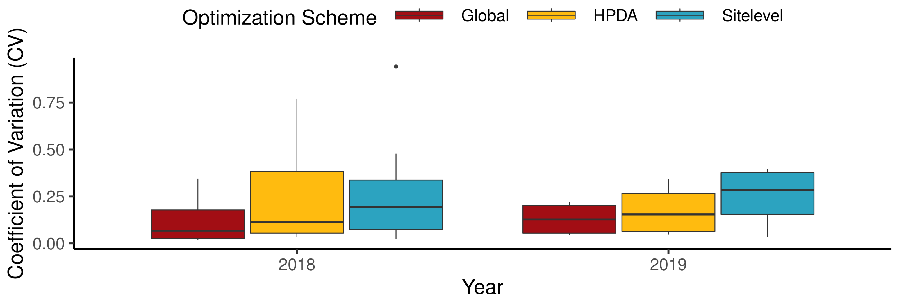

Figure A2.
Difference in the posterior distribution of parameters with LAI only, and both LAI and NDVI data constraints in HPDA.
Figure A2.
Difference in the posterior distribution of parameters with LAI only, and both LAI and NDVI data constraints in HPDA.
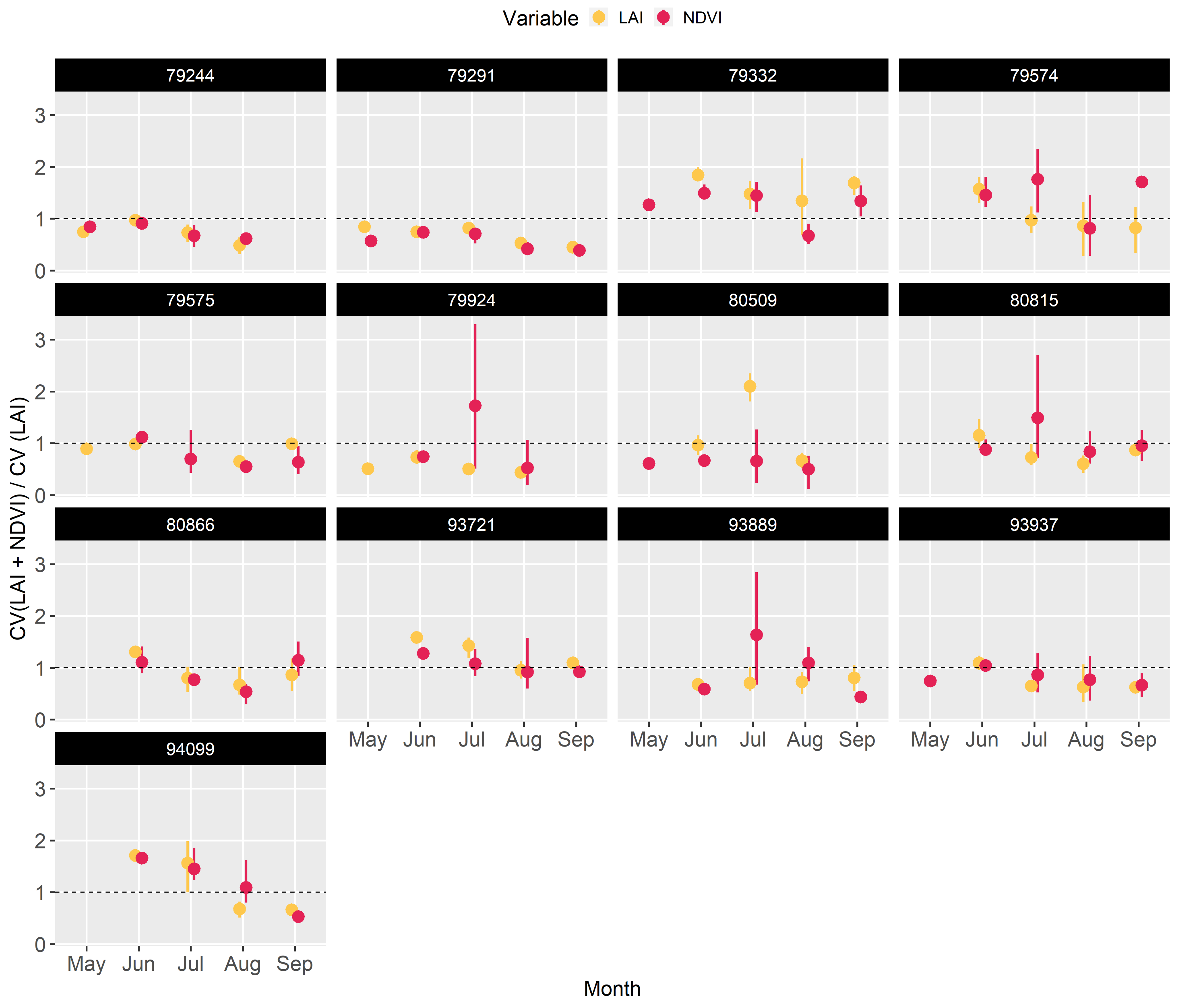

Figure A3.
95 % confidence interval for NDVI predictions made by the emulators across all the sites using the optimized parameters obtained from different optimization schemes.
Figure A3.
95 % confidence interval for NDVI predictions made by the emulators across all the sites using the optimized parameters obtained from different optimization schemes.
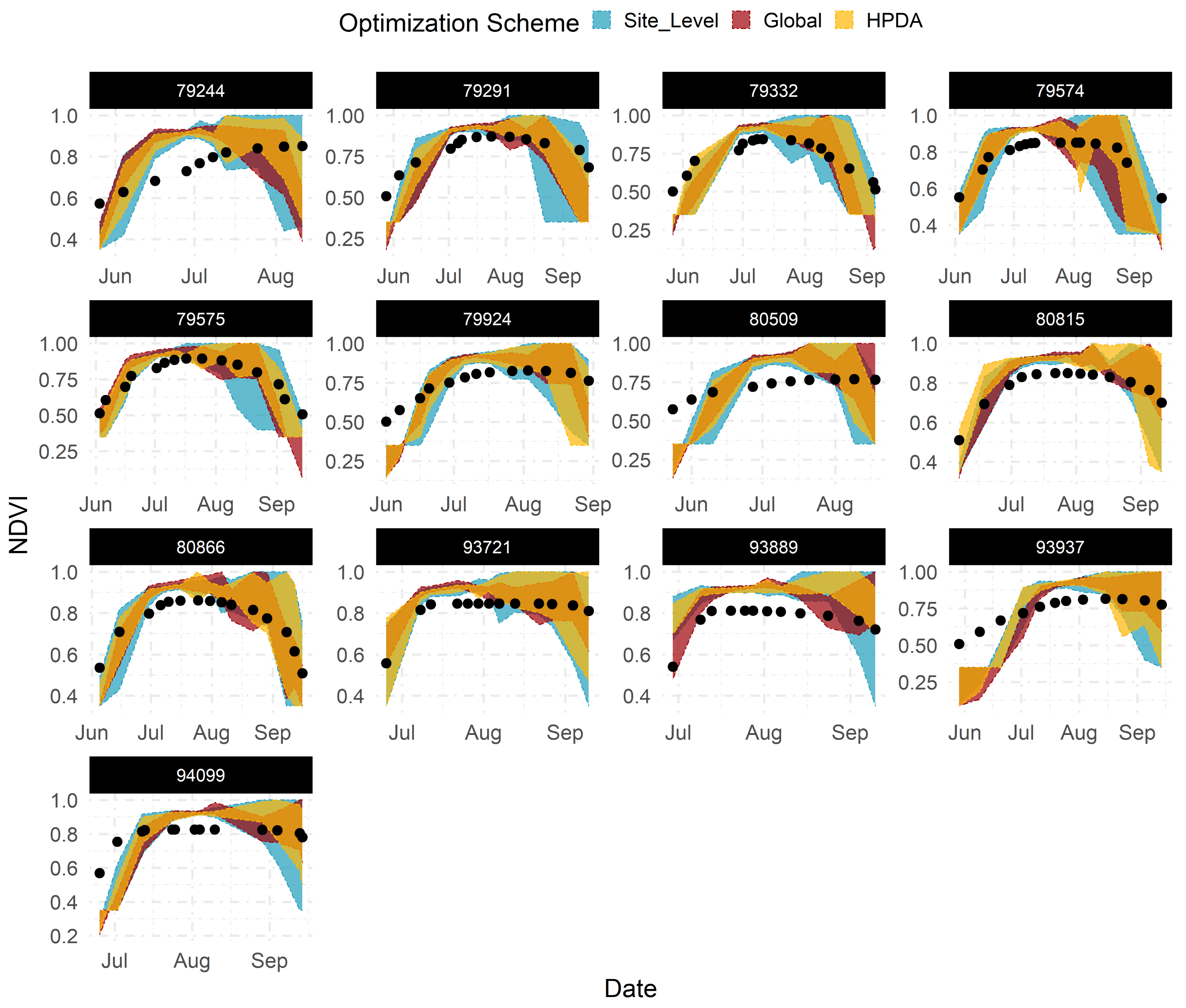

Figure A4.
Density plots comparing observed yield versus APSIM predicted maize yield for two optimization schemes.
Figure A4.
Density plots comparing observed yield versus APSIM predicted maize yield for two optimization schemes.
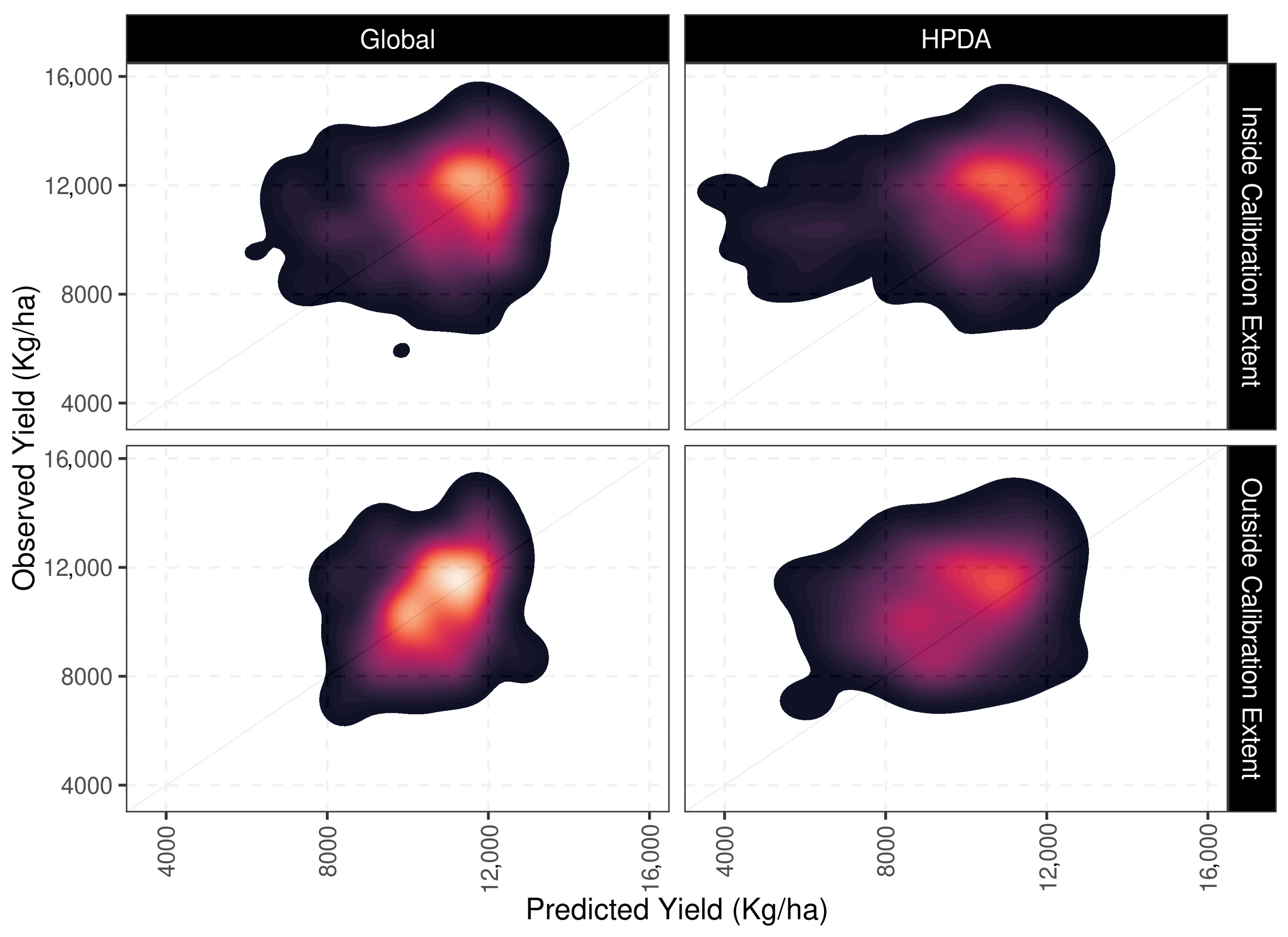

Figure A5.
Difference in the posterior distribution of parameters with LAI only and both data constraint in HPDA.
Figure A5.
Difference in the posterior distribution of parameters with LAI only and both data constraint in HPDA.
References
- Gill, H.S.; Halder, J.; Zhang, J.; Brar, N.K.; Rai, T.S.; Hall, C.; Bernardo, A.; Amand, P.S.; Bai, G.; Olson, E.; et al. Multi-Trait Multi-Environment Genomic Prediction of Agronomic Traits in Advanced Breeding Lines of Winter Wheat. Front. Plant Sci. 2021, 12, 1619. [Google Scholar] [CrossRef]
- Su, W.; Zhang, M.; Bian, D.; Liu, Z.; Huang, J.; Wang, W.; Wu, J.; Guo, H. Phenotyping of corn plants using unmanned aerial vehicle (UAV) images. Remote Sens. 2019, 11, 2021. [Google Scholar] [CrossRef]
- Dokoohaki, H.; Gheysari, M.; Mehnatkesh, A.; Ayoubi, S. Applying the CSM-CERES-Wheat model for rainfed wheat with specified soil characteristic in undulating area in Iran. Arch. Agron. Soil Sci. 2015, 61, 1231–1245. [Google Scholar] [CrossRef]
- Dietze, M. Ecological Forecasting; Princeton University Press: Princeton, NJ, USA, 2017. [Google Scholar]
- Kivi, M.S.; Blakely, B.; Masters, M.; Bernacchi, C.J.; Miguez, F.E.; Dokoohaki, H. Development of a data-assimilation system to forecast agricultural systems: A case study of constraining soil water and soil nitrogen dynamics in the APSIM model. Sci. Total Environ. 2022, 820, 153192. [Google Scholar] [CrossRef] [PubMed]
- Dokoohaki, H.; Gheisari, M.; Mousavi, S.F.; Mirlatifi, S.M. Estimation soil water content under deficit irrigation by using DSSAT. Water Irrig. Manag. 2012, 2, 1–14. [Google Scholar]
- Holzworth, D.P.; Huth, N.I.; deVoil, P.G.; Zurcher, E.J.; Herrmann, N.I.; McLean, G.; Chenu, K.; van Oosterom, E.J.; Snow, V.; Murphy, C.; et al. APSIM–evolution towards a new generation of agricultural systems simulation. Environ. Model. Softw. 2014, 62, 327–350. [Google Scholar] [CrossRef]
- Jones, J.W.; Hoogenboom, G.; Porter, C.H.; Boote, K.J.; Batchelor, W.D.; Hunt, L.; Wilkens, P.W.; Singh, U.; Gijsman, A.J.; Ritchie, J.T. The DSSAT cropping system model. Eur. J. Agron. 2003, 18, 235–265. [Google Scholar] [CrossRef]
- Archontoulis, S.V.; Castellano, M.J.; Licht, M.A.; Nichols, V.; Baum, M.; Huber, I.; Martinez-Feria, R.; Puntel, L.; Ordóñez, R.A.; Iqbal, J.; et al. Predicting crop yields and soil-plant nitrogen dynamics in the US Corn Belt. Crop Sci. 2020, 60, 721–738. [Google Scholar] [CrossRef]
- Saddique, Q.; Zou, Y.; Ajaz, A.; Ji, J.; Xu, J.; Azmat, M.; ur Rahman, M.H.; He, J.; Cai, H. Analyzing the Performance and Application of CERES-Wheat and APSIM in the Guanzhong Plain, China. Trans. ASABE 2020, 63, 1879–1893. [Google Scholar] [CrossRef]
- Rai, T.; Kumar, S.; Nleya, T.; Sexton, P.; Hoogenboom, G. Simulation of maize and soybean yield using DSSAT under long-term conventional and no-till systems. Soil Res. 2022, 60, 520–533. [Google Scholar] [CrossRef]
- Dokoohaki, H.; Kivi, M.S.; Martinez-Feria, R.A.; Miguez, F.E.; Hoogenboom, G. A comprehensive uncertainty quantification of large-scale process-based crop modeling frameworks. Environ. Res. Lett. 2021, 16, 084010. [Google Scholar] [CrossRef]
- Sun, R.; Duan, Q.; Huo, X. Multi-Objective Adaptive Surrogate Modeling-Based Optimization for Distributed Environmental Models Based on Grid Sampling. Water Resour. Res. 2021, 57, e2020WR028740. [Google Scholar] [CrossRef]
- Wallach, D.; Palosuo, T.; Thorburn, P.; Hochman, Z.; Gourdain, E.; Andrianasolo, F.; Asseng, S.; Basso, B.; Buis, S.; Crout, N.; et al. The chaos in calibrating crop models: Lessons learned from a multi-model calibration exercise. Environ. Model. Softw. 2021, 145, 105206. [Google Scholar] [CrossRef]
- Fer, I.; Gardella, A.K.; Shiklomanov, A.N.; Campbell, E.E.; Cowdery, E.M.; De Kauwe, M.G.; Desai, A.; Duveneck, M.J.; Fisher, J.B.; Haynes, K.D.; et al. Beyond ecosystem modeling: A roadmap to community cyberinfrastructure for ecological data-model integration. Glob. Chang. Biol. 2021, 27, 13–26. [Google Scholar] [CrossRef]
- Post, H.; Vrugt, J.A.; Fox, A.; Vereecken, H.; Hendricks Franssen, H.J. Estimation of Community Land Model parameters for an improved assessment of net carbon fluxes at European sites. J. Geophys. Res. Biogeosci. 2017, 122, 661–689. [Google Scholar] [CrossRef]
- Fer, I.; Shiklomanov, A.N.; Novick, K.A.; Gough, C.M.; Arain, M.A.; Chen, J.; Murphy, B.; Desai, A.R.; Dietze, M.C. Capturing site-to-site variability through Hierarchical Bayesian calibration of a process-based dynamic vegetation model. bioRxiv 2021. [Google Scholar] [CrossRef]
- Dokoohaki, H.; Morrison, B.D.; Raiho, A.; Serbin, S.P.; Zarada, K.; Dramko, L.; Dietze, M. Development of an open-source regional data assimilation system in PEcAn v. 1.7. 2: Application to carbon cycle reanalysis across the contiguous US using SIPNET. Geosci. Model Dev. Discuss. 2022, 15, 1–28. [Google Scholar] [CrossRef]
- Huang, J.; Gómez-Dans, J.L.; Huang, H.; Ma, H.; Wu, Q.; Lewis, P.E.; Liang, S.; Chen, Z.; Xue, J.H.; Wu, Y.; et al. Assimilation of remote sensing into crop growth models: Current status and perspectives. Agric. For. Meteorol. 2019, 276, 107609. [Google Scholar] [CrossRef]
- Jacquemoud, S.; Baret, F. PROSPECT: A model of leaf optical properties spectra. Remote Sens. Environ. 1990, 34, 75–91. [Google Scholar] [CrossRef]
- Shiklomanov, A.N.; Dietze, M.C.; Fer, I.; Viskari, T.; Serbin, S.P. Cutting out the middleman: Calibrating and validating a dynamic vegetation model (ED2-PROSPECT5) using remotely sensed surface reflectance. Geosci. Model Dev. 2021, 14, 2603–2633. [Google Scholar] [CrossRef]
- Dokoohaki, H.; Miguez, F.E.; Archontoulis, S.; Laird, D. Use of inverse modelling and Bayesian optimization for investigating the effect of biochar on soil hydrological properties. Agric. Water Manag. 2018, 208, 268–274. [Google Scholar] [CrossRef]
- Akhavizadegan, F.; Ansarifar, J.; Wang, L.; Huber, I.; Archontoulis, S.V. A time-dependent parameter estimation framework for crop modeling. Sci. Rep. 2021, 11, 1–15. [Google Scholar]
- Dietzel, R.; Liebman, M.; Ewing, R.; Helmers, M.; Horton, R.; Jarchow, M.; Archontoulis, S. How efficiently do corn-and soybean-based cropping systems use water? A systems modeling analysis. Glob. Chang. Biol. 2016, 22, 666–681. [Google Scholar] [CrossRef] [PubMed]
- Sheng, M.; Liu, J.; Zhu, A.X.; Rossiter, D.G.; Liu, H.; Liu, Z.; Zhu, L. Comparison of GLUE and DREAM for the estimation of cultivar parameters in the APSIM-maize model. Agric. For. Meteorol. 2019, 278, 107659. [Google Scholar] [CrossRef]
- Malone, R.W.; Huth, N.; Carberry, P.; Ma, L.; Kaspar, T.C.; Karlen, D.L.; Meade, T.; Kanwar, R.S.; Heilman, P. Evaluating and predicting agricultural management effects under tile drainage using modified APSIM. Geoderma 2007, 140, 310–322. [Google Scholar] [CrossRef]
- Archontoulis, S.V.; Miguez, F.E.; Moore, K.J. Evaluating APSIM maize, soil water, soil nitrogen, manure, and soil temperature modules in the Midwestern United States. Agron. J. 2014, 106, 1025–1040. [Google Scholar] [CrossRef]
- Puntel, L.A.; Sawyer, J.E.; Barker, D.W.; Dietzel, R.; Poffenbarger, H.; Castellano, M.J.; Moore, K.J.; Thorburn, P.; Archontoulis, S.V. Modeling long-term corn yield response to nitrogen rate and crop rotation. Front. Plant Sci. 2016, 7, 1630. [Google Scholar] [CrossRef]
- Ojeda, J.J.; Volenec, J.J.; Brouder, S.M.; Caviglia, O.P.; Agnusdei, M.G. Modelling stover and grain yields, and subsurface artificial drainage from long-term corn rotations using APSIM. Agric. Water Manag. 2018, 195, 154–171. [Google Scholar] [CrossRef]
- Basche, A.D.; Archontoulis, S.V.; Kaspar, T.C.; Jaynes, D.B.; Parkin, T.B.; Miguez, F.E. Simulating long-term impacts of cover crops and climate change on crop production and environmental outcomes in the Midwestern United States. Agric. Ecosyst. Environ. 2016, 218, 95–106. [Google Scholar] [CrossRef]
- USDA National Agricultural Statistics Service. NASS—Quick Stats. USDA National Agricultural Statistics Service. Available online: https://data.nal.usda.gov/dataset/nass-quick-stats (accessed on 20 November 2021).
- Kang, Y.; Özdoğan, M. Field-level crop yield mapping with Landsat using a hierarchical data assimilation approach. Remote Sens. Environ. 2019, 228, 144–163. [Google Scholar] [CrossRef]
- Hengl, T.; Mendes de Jesus, J.; Heuvelink, G.B.; Ruiperez Gonzalez, M.; Kilibarda, M.; Blagotić, A.; Shangguan, W.; Wright, M.N.; Geng, X.; Bauer-Marschallinger, B.; et al. SoilGrids250m: Global gridded soil information based on machine learning. PLoS ONE 2017, 12, e0169748. [Google Scholar] [CrossRef] [PubMed]
- Hersbach, H.; Bell, B.; Berrisford, P.; Hirahara, S.; Horányi, A.; Muñoz-Sabater, J.; Nicolas, J.; Peubey, C.; Radu, R.; Schepers, D.; et al. The ERA5 global reanalysis. Q. J. R. Meteorol. Soc. 2020, 146, 1999–2049. [Google Scholar] [CrossRef]
- Bolton, D.K.; Friedl, M.A. Forecasting crop yield using remotely sensed vegetation indices and crop phenology metrics. Agric. For. Meteorol. 2013, 173, 74–84. [Google Scholar] [CrossRef]
- Jacquemoud, S.; Verhoef, W.; Baret, F.; Bacour, C.; Zarco-Tejada, P.J.; Asner, G.P.; François, C.; Ustin, S.L. PROSPECT+ SAIL models: A review of use for vegetation characterization. Remote Sens. Environ. 2009, 113, S56–S66. [Google Scholar] [CrossRef]
- Müller, C.; Elliott, J.; Kelly, D.; Arneth, A.; Balkovic, J.; Ciais, P.; Deryng, D.; Folberth, C.; Hoek, S.; Izaurralde, R.C.; et al. The Global Gridded Crop Model Intercomparison phase 1 simulation dataset. Sci. Data 2019, 6, 50. [Google Scholar] [CrossRef]
- Martinez-Feria, R.; Nichols, V.; Basso, B.; Archontoulis, S. Can multi-strategy management stabilize nitrate leaching under increasing rainfall? Environ. Res. Lett. 2019, 14, 124079. [Google Scholar] [CrossRef]
- Keating, B.A.; Carberry, P.S.; Hammer, G.L.; Probert, M.E.; Robertson, M.J.; Holzworth, D.; Huth, N.I.; Hargreaves, J.N.; Meinke, H.; Hochman, Z.; et al. An overview of APSIM, a model designed for farming systems simulation. Eur. J. Agron. 2003, 18, 267–288. [Google Scholar] [CrossRef]
- Birch, C.; Hammer, G.; Rickert, K. Improved methods for predicting individual leaf area and leaf senescence in maize (Zea mays). Aust. J. Agric. Res. 1998, 49, 249–262. [Google Scholar] [CrossRef]
- Jones, C.A. CERES-Maize; a Simulation Model of Maize Growth and Development; Number 04; SB91. M2, J6.; Texas A&M University Press: College Station, TX, USA, 1986. [Google Scholar]
- Keating, B.; Wafula, B. Modelling the fully expanded area of maize leaves. Field Crop. Res. 1992, 29, 163–176. [Google Scholar] [CrossRef]
- Machwitz, M.; Giustarini, L.; Bossung, C.; Frantz, D.; Schlerf, M.; Lilienthal, H.; Wandera, L.; Matgen, P.; Hoffmann, L.; Udelhoven, T. Enhanced biomass prediction by assimilating satellite data into a crop growth model. Environ. Model. Softw. 2014, 62, 437–453. [Google Scholar] [CrossRef]
- Duan, S.B.; Li, Z.L.; Wu, H.; Tang, B.H.; Ma, L.; Zhao, E.; Li, C. Inversion of the PROSAIL model to estimate leaf area index of maize, potato, and sunflower fields from unmanned aerial vehicle hyperspectral data. Int. J. Appl. Earth Obs. Geoinf. 2014, 26, 12–20. [Google Scholar] [CrossRef]
- Richter, K.; Atzberger, C.; Vuolo, F.; D’Urso, G. Evaluation of sentinel-2 spectral sampling for radiative transfer model based LAI estimation of wheat, sugar beet, and maize. IEEE J. Sel. Top. Appl. Earth Obs. Remote Sens. 2010, 4, 458–464. [Google Scholar] [CrossRef]
- Fer, I.; Kelly, R.; Moorcroft, P.R.; Richardson, A.D.; Cowdery, E.M.; Dietze, M.C. Linking big models to big data: Efficient ecosystem model calibration through Bayesian model emulation. Biogeosciences 2018, 15, 5801–5830. [Google Scholar] [CrossRef]
- De Valpine, P.; Turek, D.; Paciorek, C.J.; Anderson-Bergman, C.; Lang, D.T.; Bodik, R. Programming with models: Writing statistical algorithms for general model structures with NIMBLE. J. Comput. Graph. Stat. 2017, 26, 403–413. [Google Scholar] [CrossRef]
- Dokoohaki, H.; Gheysari, M.; Mousavi, S.F.; Hoogenboom, G. Effects of different irrigation regimes on soil moisture availability evaluated by CSM-CERES-Maize model under semi-arid condition. Ecohydrol. Hydrobiol. 2017, 17, 207–216. [Google Scholar] [CrossRef]
- Pasley, H.; Nichols, V.; Castellano, M.; Baum, M.; Kladivko, E.; Helmers, M.; Archontoulis, S. Rotating maize reduces the risk and rate of nitrate leaching. Environ. Res. Lett. 2021, 16, 064063. [Google Scholar] [CrossRef]
- Martinez-Feria, R.A.; Licht, M.A.; Ordóñez, R.A.; Hatfield, J.L.; Coulter, J.A.; Archontoulis, S.V. Evaluating maize and soybean grain dry-down in the field with predictive algorithms and genotype-by-environment analysis. Sci. Rep. 2019, 9, 7167. [Google Scholar] [CrossRef]
- Dos Santos, C.L.; Abendroth, L.J.; Coulter, J.A.; Nafziger, E.D.; Suyker, A.; Yu, J.; Schnable, P.S.; Archontoulis, S.V. Maize Leaf Appearance Rates: A Synthesis From the United States Corn Belt. Front. Plant Sci. 2022, 13, 872738. [Google Scholar] [CrossRef]
- Clark, J.S. Why environmental scientists are becoming Bayesians. Ecol. Lett. 2005, 8, 2–14. Available online: http://xxx.lanl.gov/abs/https://onlinelibrary.wiley.com/doi/pdf/10.1111/j.1461-0248.2004.00702.x (accessed on 20 November 2021). [CrossRef]
- Van Oijen, M. Bayesian methods for quantifying and reducing uncertainty and error in forest models. Curr. For. Rep. 2017, 3, 269–280. [Google Scholar] [CrossRef]
- Oberpriller, J.; Cameron, D.R.; Dietze, M.C.; Hartig, F. Towards robust statistical inference for complex computer models. Ecol. Lett. 2021, 24, 1251–1261. [Google Scholar] [CrossRef] [PubMed]
- Cressie, N.; Calder, C.A.; Clark, J.S.; Hoef, J.M.V.; Wikle, C.K. Accounting for uncertainty in ecological analysis: The strengths and limitations of hierarchical statistical modeling. Ecol. Appl. 2009, 19, 553–570. [Google Scholar] [CrossRef] [PubMed]
- Sexton, J.; Everingham, Y.; Inman-Bamber, G. A theoretical and real world evaluation of two Bayesian techniques for the calibration of variety parameters in a sugarcane crop model. Environ. Model. Softw. 2016, 83, 126–142. [Google Scholar] [CrossRef]
- Makowski, D.; Wallach, D.; Tremblay, M. Using a Bayesian approach to parameter estimation; comparison of the GLUE and MCMC methods. Agronomie 2002, 22, 191–203. [Google Scholar] [CrossRef]
- Gao, F.; Zhang, X. Mapping crop phenology in near real-time using satellite remote sensing: Challenges and opportunities. J. Remote Sens. 2021, 2021, 8379391. [Google Scholar] [CrossRef]
- Pearson, N.C.; Livo, K.E.; Driscoll, R.L.; Lowers, H.A.; Hoefen, T.M.; Swayze, G.A.; Klein, A.J.; Kokaly, R.F.; Wise, R.A.; Benzel, W.M.; et al. USGS Spectral Library Version 7 Data. 2017. Available online: https://dx.doi.org/10.5066/F7RR1WDJ (accessed on 3 March 2020).
- Garrity, D.; Bindraban, P. A Globally Distributed Soil Spectral Library Visible Near Infrared Diffuse Reflectance Spectra; ICRAF (World Agroforestry Centre)/ISRIC (World Soil Information) Spectral Library: Nairobi, Kenya, 2004. [Google Scholar]
- Price, J.C. On the information content of soil reflectance spectra. Remote Sens. Environ. 1990, 33, 113–121. [Google Scholar] [CrossRef]
Publisher’s Note: MDPI stays neutral with regard to jurisdictional claims in published maps and institutional affiliations. |
© 2022 by the authors. Licensee MDPI, Basel, Switzerland. This article is an open access article distributed under the terms and conditions of the Creative Commons Attribution (CC BY) license (https://creativecommons.org/licenses/by/4.0/).

