On Tide Aliasing in GRACE Time-Variable Gravity Observations

Abstract

Aliasing error induced by tide-related high frequency mass variations is one of the most significant errors in the Gravity Recovery and Climate Experiment (GRACE). In the present work, we evaluated the 161.0-day S₂, 171.2-day P₁, and 322.1-day S₁ ocean tide aliasing in GRACE latest RL06 data based on nearly 15 years of observation from 2002 to 2017. Tide aliasing was still obvious for current GRACE observations, especially for S₂ and P₁ aliasing. S₂ aliasing was mostly evident over West Antarctica, and was a clearly eastward propagation that travelled around Antarctica in about 2 years, while P₁ showed strongest aliasing over South Greenland. More seriously, we found that GRACE mascon data showed an extremely large aliasing error. The mascon data may have unintentionally amplified the aliasing error on land due to the regularization (or constraint) applied for reducing signal leakage. Enough attention must be paid to tide aliasing when using GRACE for assessing mass variations at high latitudes (e.g., glaciers in polar regions) which can cause potential obstacles to estimation of actual seasonality.

1. Introduction

Since its launch in 2002, the GRACE satellite mission has opened up a new way to observe the Earth’s global mass transport by providing monthly records of global time-variable gravity (TVG) field solutions [1,2]. The monthly temporal resolution satisfies the majority of the TVG signals with long-period variability including the dominant seasonal or interannual time scales. However, well-known signal aliasing errors prevail in shorter-period mass variations, most often over the Earth’s surface [3], due to GRACE’s incomplete sampling in both space and time domains [4], that must be removed by appropriate geophysical models.

To acquire all essential information, a discrete signal resampled from a continuous signal should satisfy the Nyquist–Shannon theorem [5], $f_s>2f$, where $f_s$ is the sampling frequency and $f$ is the frequency of the original continuous signal. Otherwise, a high-frequency signal will map into lower frequency due to the incomplete sampling and result in sampling a false signal with longer period. Aliasing in satellite gravimetry is induced by a more complicated two-step mechanism [6]. The primary aliasing is caused by orbit under-sampling of original high frequency signals and the secondary aliasing is due to under-sampling of the primary aliasing signals through gravity recovery in discrete (monthly) time intervals.

The monthly temporal resolution of GRACE does not meet some Earth-surface physical processes with high frequency, for example, (i) substantial non-tidal mass variations with a period below 30 days, e.g., heavy precipitation events in a short period of time, can occasionally induce a rapid increase of the water stored on the continents [7] and (ii) surface mass redistribution caused by diurnal and semi-diurnal lunar and solar tides with periods of 24 h and 12 h [8]. These processes can lead to potential aliasing of GRACE observations and will obscure the more subtle climate signals which are the focus of GRACE. While the former can reasonably well be removed by Atmosphere and Ocean De-Aliasing Level-1B [7] products, aliasing induced by the tides is particularly tricky. The current tidal models are imperfect [8,9,10], especially for high latitudes where there is a lack of tide observation. Errors in tidal models could produce mismodeling of tidal and atmospheric perturbations on the monthly mean gravity-field estimates [3].

The GRACE tide problem has been previously addressed by number of studies, both before launch and subsequently. For example, Knudsen et al. [11] pointed out that the tide aliasing will not cancel in the GRACE monthly averaged temporal gravity fields unless modeled by the appropriate tidal models. Using the 5-day temporal resolution GRACE satellite-to-satellite tracking data, Han et al. [12] recognized the 13.6-day M₂ and 161.0-day S₂ tide aliasing over Antarctica. Chen et al. [13] further examine the S₂ tide aliasing in GRACE RL01 and RL04 versions, and showed evident aliasing at high latitudes where tide observations by satellite altimetry and tide gauges are relatively sparse. Meanwhile, significant tide aliasing was also found in GRACE low-degree Stokes coefficients caused by errors in ocean tidal models [14]. However, tide aliasing in current GRACE RL06 data is yet to be understood. In addition, since the release of the GRACE level-3 mascon data, there is a crying need for an evaluation of its aliasing effect.

The phase-sampling of tide is controlled by the precession rate ${\mathsf{\Omega }}_G$of the GRACE orbit plane relative to the tide-raising body [10]. For any tidal constituent there is a fictitious moon circling the Earth with frequency ${\mathsf{\Theta }}_E-f/m$, where $f$ is the constituent frequency, $m$ is the tidal species, and ${\mathsf{\Theta }}_E$ is the Earth’s sidereal rotation rate. The alias frequency is then $f_{alias}=\left|m\left({\mathsf{\Theta }}_E-{\mathsf{\Omega }}_G\right)-f\right|$.

Table 1. Tide constituents and their alias period in days.

Tide Constituents	Cause	Alias Period (Days)
Q1	Moon	9.1
M2	Moon	13.6
N2	Moon	9.1
J1	Moon	27.8
S2	Sun	161.0
P1	Sun	171.2
S1	Sun	322.1
K2	Moon + Sun	1362.7
K1	Moon + Sun	2725.4

lists the aliasing periods of individual tide constituents, and their contributions to specific spherical harmonic coefficients of arbitrary degree, and order can be seen in Cartwright and Tayler [15]. Aliasing periods of less than 30 days (Q₁, M₂, N₂, J₁) could not have a significant impact on GRACE monthly time-variable gravity solutions [16], and can be ignored. Aliasing with longer periods such as the K₁ and K₂ is not within the scope of this work. These periods are much more difficult to estimate at present with the limited 15 years’ GRACE data accumulation. Here, we mainly focus on the 161.0-day S₂, 171.2-day P₁, and 322.1-day S₁ tide aliasing in GRACE data.

2. Materials

The level-2 spherical harmonic (SH) products provided by the Center for Space Research (CSR), GeoForschungsZentrum (GFZ) and Jet Propulsion Laboratory (JPL), and the level-3 mascon products provided by CSR and JPL were both investigated. The GRACE data used in the study spanned from 2002 to 2017, and consisted of 163 monthly global “maps” that covered all GRACE observations during this period.

For SH data, because GRACE satellites do not provide degree-1 coefficients, the spherical-harmonic degree-1 coefficients (i.e., geocenter) were treated in accordance with Swenson et al.’s estimates [17]. The submitted C₂₀ harmonic coefficients were derived from the satellite laser ranging [18]. A glacial isostatic adjustment correction was applied according to the model ICE6G-D [19]. Necessary post-processing was also required for SH solutions when converting the time-variable gravity to mass change. A 300 km Gaussian filter was applied to suppress noise in high-degree and order coefficients. Generally a larger radius will further reduce the noise, but the signal will also be greatly attenuated (e.g., [20]), thus a more conservative radius was selected here. Furthermore, a decorrelation filter denoted P4M6 [21] was adopted to reduce the longitudinal stripes in GRACE data. The filtered coefficients were then converted to a 1/4-degree latitude–longitude global mass grid in the form of the equivalent water height (EWH).

Differing from the SH data, mascon data is a direct product of the GRACE observations that relate to the L1B range–rate or the range–acceleration data [22]. The CSR mascon solution inverses surface-mass changes by time-variable Tikhonov regularization matrices [23], while the JPL mascon uses a priori constraints in space and time to estimate global, monthly gravity fields in terms of equal-area spherical cap mass concentration functions to minimize the effect of measurement errors [23]. The conducted data pre-processing, such as replacement of low-degree coefficients and glacial isostatic adjustment correction (ICE6G-D model), ensured that the mascon solution could be used directly. The mascon data was provided in the form of EWH in cm units on a 1/4-degree grid for the CSR mascon, and a 1/2-degree grid for the JPL mascon.

It should be pointed out that the time-variable mass signals obtained from GRACE (either SH-based or mascon mass signals) are under the assumption that the gravity signals are generated only by mass transports that occur on the Earth’s surface. It would be a “mistake” to convert gravity (in the form of the Stokes coefficient) to mass, because that gravity-to-mass “conversion” is impossible in 3-D under the well-known non-uniqueness of the gravitational inversion [24]. This is possible only if one assumes that all gravity (or gravity change in the case of GRACE) comes from the surface (so that 3-D becomes 2-D), an assumption with which we have abided with respect to the target phenomena in this paper.

3. Results

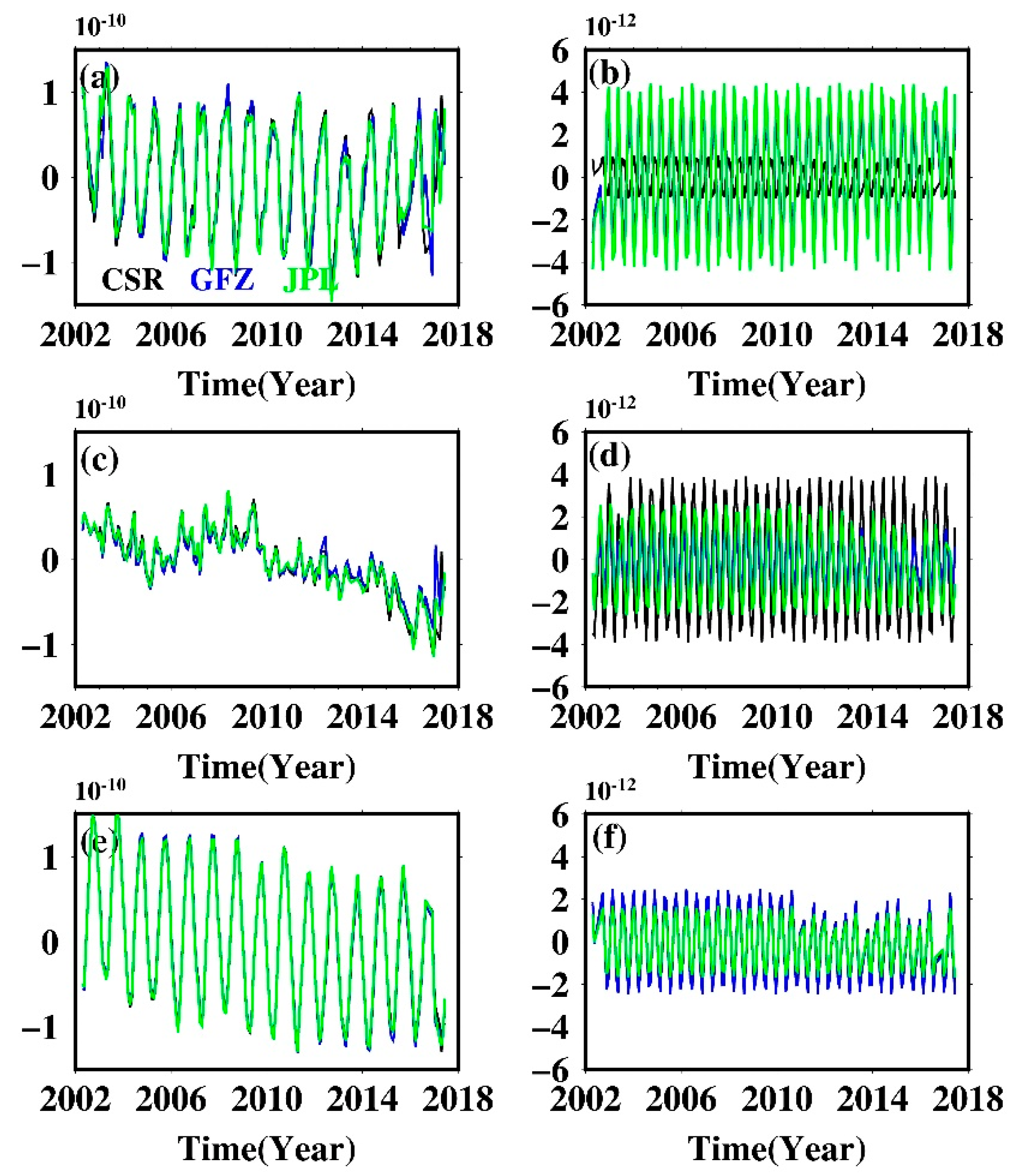
3.1. Tide Aliasing in Low-Degree Stokes Coefficients

The S₂ semi-diurnal tide will produce long-period variations in order 2 Stokes coefficients, C_n2/S_n2, while the P₁ and S₁ diurnal tide will alias in C_n1/S_n1 [25]. We mainly focused on C₂₂/S₂₂ and C₂₁/S₂₁, coefficients that are the most sensitive to tide perturbations. Higher-degree coefficients can be also affected by tide aliasing of course, but the magnitude of the perturbation will be greatly attenuated with increasing degree [26]. Figure 1 shows the non-secular, non-seasonal time series of Stokes coefficients C₂₁/S₂₁ and C₂₂/S₂₂, as well as their conventional discrete Fourier spectrum, derived from CSR, GFZ, and JPL SH solutions. S₁ aliasing in C₂₁/S₂₁ is evident for all datasets, and coefficients from GFZ are more susceptible to its disturbance compared with that of CSR and JPL, as judged from their normalized power series. P₁ aliasing is virtually unnoticeable in C₂₁/S₂₁ coefficients; only GFZ’s C21 coefficient shows weak P₁ aliasing. S₂ aliasing is widely presented in C₂₂/S₂₂ and is also much pronounced for GFZ data. Low-degree coefficients clearly show the impact of tide aliasing on GRACE data and reveal that the new tidal models adopted in the RL06 version do not perfectly simulate the actual tides.

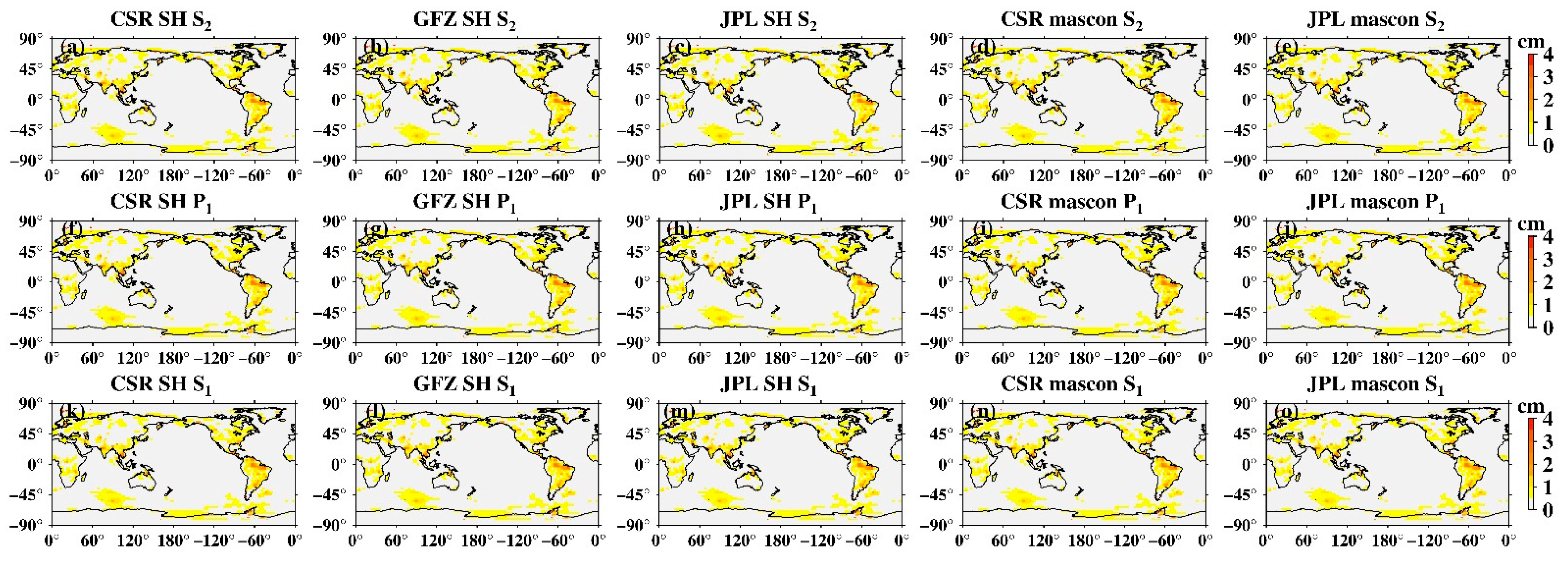
3.2. Global Amplitude of the Tide Aliasing Signal

Unlike low-degree coefficients, high degree coefficients are also influenced by tide aliasing [16], we thus investigated the spatial distribution of tide aliasing using Stokes coefficients up to degree and order 60. Mascon solutions provided by CSR and JPL were also investigated. At each grid, we used the least-square-fit linear trends and amplitudes of annual, semi-annual, 161.0-day S₂, 171.2-day P₁, and 322.1-day S₁ aliasing signals. Figure 2 presents the global amplitudes of S₂, P₁, and S₁ aliasing. The S₂ tide aliasing in SH solutions (Figure 2a–c) is most obviously at high latitudes, particularly regions over West Antarctica. A few tropical oceans show stripe-like S₂ aliasing. In particular, oceans around North-West Australia, may reflect the deficiencies of the ocean tidal models [27]. Moreover, some land regions, e.g., the Amazon River basin also shows noticeable amplitudes, possibly due to errors in the S₂ atmospheric tide [28], or nonseasonal hydrology variations [13]. Those results are consistent with what has reported based on previous GRACE RL01 and RL04 versions (e.g., [12,13,14]), delivering the gloomy fact that there is no essential improvement with the latest RL06 version in suppression of S₂ tide aliasing. The S₂ tide aliasing in mascon data (Figure 2d,e) has certain features that are clearly different from SH data. S₂ aliasing over tropical oceans in mascon solutions has greatly reduced, however, its amplitudes over polar oceans are much greater, e.g., the Arctic Ocean and the Weddell Sea near West Antarctica. In addition, S₂ aliasing over West Antarctica and peripheral Greenland is much larger than SH data (for detail see Section 3.3 and Section 3.4).

Not surprisingly, the amplitudes of P₁ (Figure 2f,g) and S₁ aliasing (Figure 2k–o) are significantly smaller than S₂, because diurnal tides along the ascending and descending GRACE orbits are roughly opposite in phase and therefore mostly cancel in monthly gravity field solutions [10]. They have almost no influence on GRACE observations for most areas, only mascon data shows relatively large amplitudes over the Amazon River basin and South Greenland (Figure 2i,j,n,o). We also did the same analysis for the monthly ITSG solutions [29]. These performed quite well especially for S₂ and P₁ aliasing, only showing relatively large S₁ amplitudes over large-scale basins such as the Amazon basin and South Africa, which may have represented non-seasonal changes of terrestrial water storage (for detail see, Figure S1 in Supplemental Materials).

The above analyses suggest that tide-aliasing errors still exist in the latest GRACE data, especially S₂ tide aliasing. For whatever known reason, aliasing in mascon data is much pronounced than SH data, particularly for Antarctica and Greenland. It will be a tricky situation when the aliasing gets under the ice shelves because the aliasing error will interweave with the actual ice-mass variations, and it will be hard to separate them effectively. We shall focus on Antarctica and Greenland, where the strongest tide aliasing can be seen.

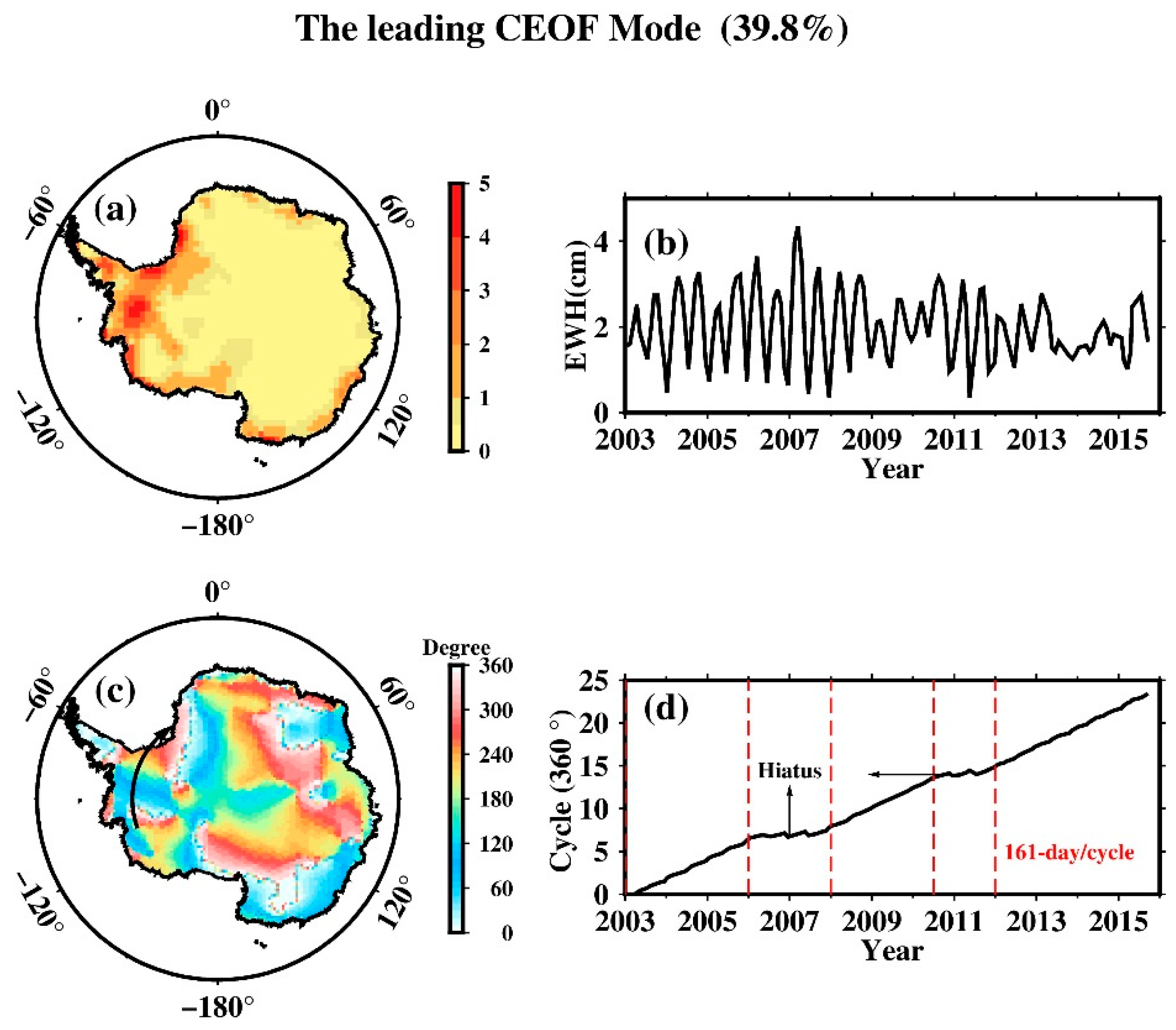
3.3. Tide Aliasing over Antarctica

Figure 3 presents the spatial amplitude maps of S₂ aliasing over Antarctica estimated from GRACE SH and mascon datasets, as well as their corresponding phase maps. All datasets share basically similar results. West Antarctica shows the strongest amplitude, particular for regions near the Ronne ice shelve. For SH solutions, the largest amplitudes are 3.1 cm (CSR), 2.6 cm (GFZ), and 3.5 cm (JPL), respectively, after spatial smoothing and de-stripping (see above). For mascon solutions, although the spatial distribution is consistent with that of SH, it mostly concentrates along West Antarctica; however, the amplitude is unexpectedly large. The maximum amplitude of the CSR mascon is 17.2 cm while the JPL mascon is, incredibly, 83.4 cm. Such amplitudes are too large to be reasonable, suggesting the S₂ aliasing in mascon data is indeed a serious error.

Errors in tidal models can propagate globally as resonant errors through correlations with satellite state, accelerometer, and range–rate parameters estimated during the orbit determination and accelerometer calibration process [10]. S₂ tide aliasing is a clear propagating wave that travels along Antarctica continent as judged from the phase map in Figure 3. To reveal the nature of its propagation, we employed the EOF (empirical orthogonal function) and CEOF (complex EOF) method (e.g., [30,31,32]) on the non-secular, non-seasonal, interannual GRACE observations over Antarctica. Because all the datasets have a similar phase map, we only did principal component analysis on the CSR mascon solution. We mainly focused on the time spans of 2003 to 2015, in which GRACE had high-quality observations with less error. We first removed the secular quadratic trend and the seasonal signals (including annual and semi-annual terms) from the data via linear least-squares regression. The residual time series constituted the target dataset to be inputted into the analyses below, yielding output solutions shown in Figure 4. We mainly focused on the EOF Modes 2–4, since the leading EOF mode has been identified as representing the physically distinct standing-wave phenomenon of the Antarctica Coastal Dipole (ACD) [32]. EOF Modes 2–4 shared some rather similar properties: (i) the respective percentage variances were rather close in value, at 20.7%, 17.2%, and 16.0%; (ii) the spatial functions exhibited similar patterns that concentrated along West Antarctica; (iii) the time functions all showed prominent intraseasonal quasi-periodicity of ~161 day (see Figure 5 of their time–frequency wavelet spectra). That is the true nature of the S₂ propagating wave that have seen in the phase map. We thus invoked a CEOF analysis to further reveal its nature of propagation.

The leading CEOF mode after removal of the ACD, now explains as much as 39.8% of the total variance. West Antarctica has the strongest spatial patterns in terms of root-mean-square amplitude (Figure 6a). The corresponding time series (Figure 6b) shows strong undulation at the clear quasi-semiannual periodicity in the (absolute) amplitude. This represents the 161.0-day modulation of the overall amplitude of the EOFs. The S propagation is clearly delineated in the spatial phase map (Figure 6c) which shows a clockwise spin as viewed from over the South Pole, or an eastward propagation around Antarctica, particularly in West Antarctica. The period (time duration for making a 360° cycle of phase) of the propagation had undergone an interesting scenario that can be discerned from the slope of the (unwrapped) phase time series in Figure 6d. During the 3 years of 2003–2005 this propagating mode had an average period of ~161 days per cycle, then paused (not vanished) as hiatus (staying stationary) for 2 years of 2006–2007, resumed at period of ~161 days per cycle for 2.5 years of 2008–2010.5, paused for another year during 2010.5–2012, then resumed again at period of ~161 days per cycle from 2012 till the end of dataset. In terms of geographical distance traversed, it can be estimated from Figure 6c,d that the S2 tide aliasing completes a full clockwise/eastward circuit around Antarctica in about 2 years.

The amplitudes of P₁ and S₁ over Antarctica (Figure 7 and Figure 8) are relatively weak compared with S₂. They are barely noticeable in SH solutions (less than 1.5 cm for most regions both for P₁ and S₁), but relatively large amplitudes appear in mascon solutions. The maximum amplitude of P₁ for the CSR mascon is 5.2 cm, and 3.7 cm for the JPL mascon. There is a similar situation for S₁, with the maximum amplitude for the CSR mascon being 5.9 cm and 6.7 cm for the JPL mascon, showing that the P₁ and S₁ aliasing are amplified about 3–5 times in mascon solutions.

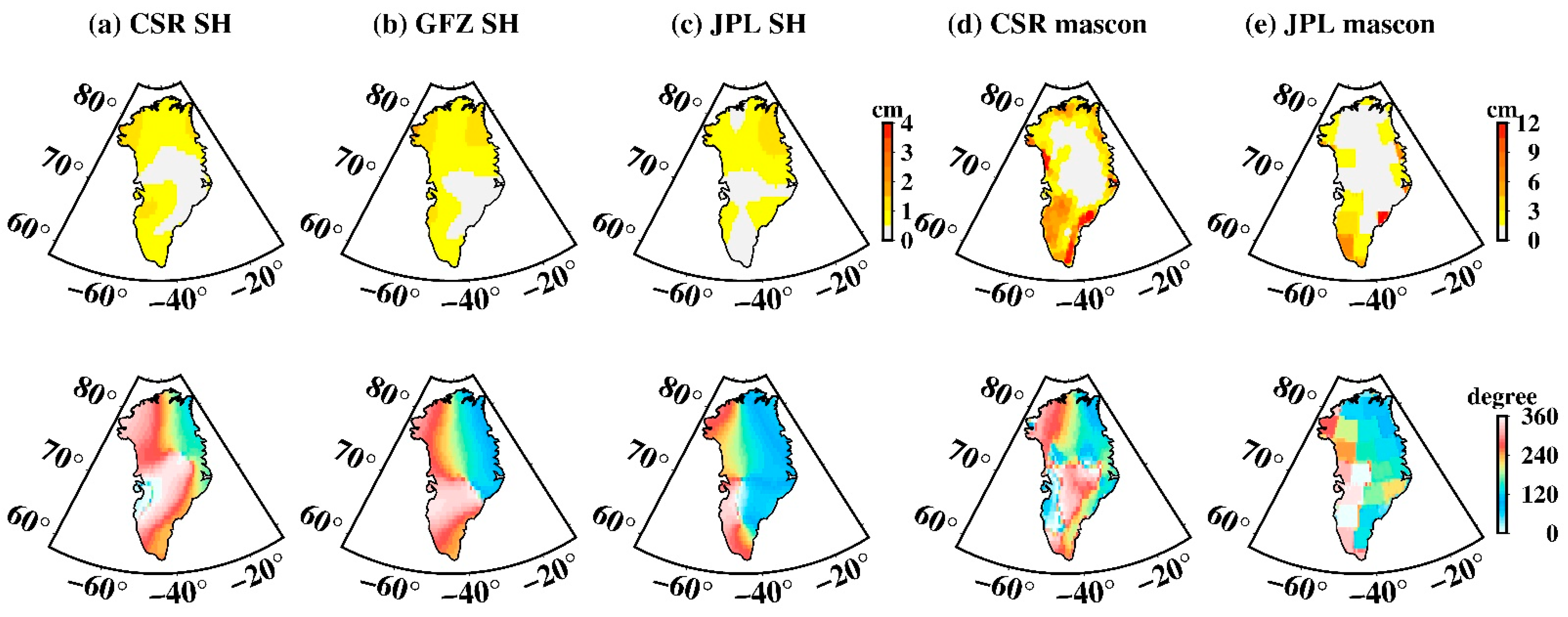
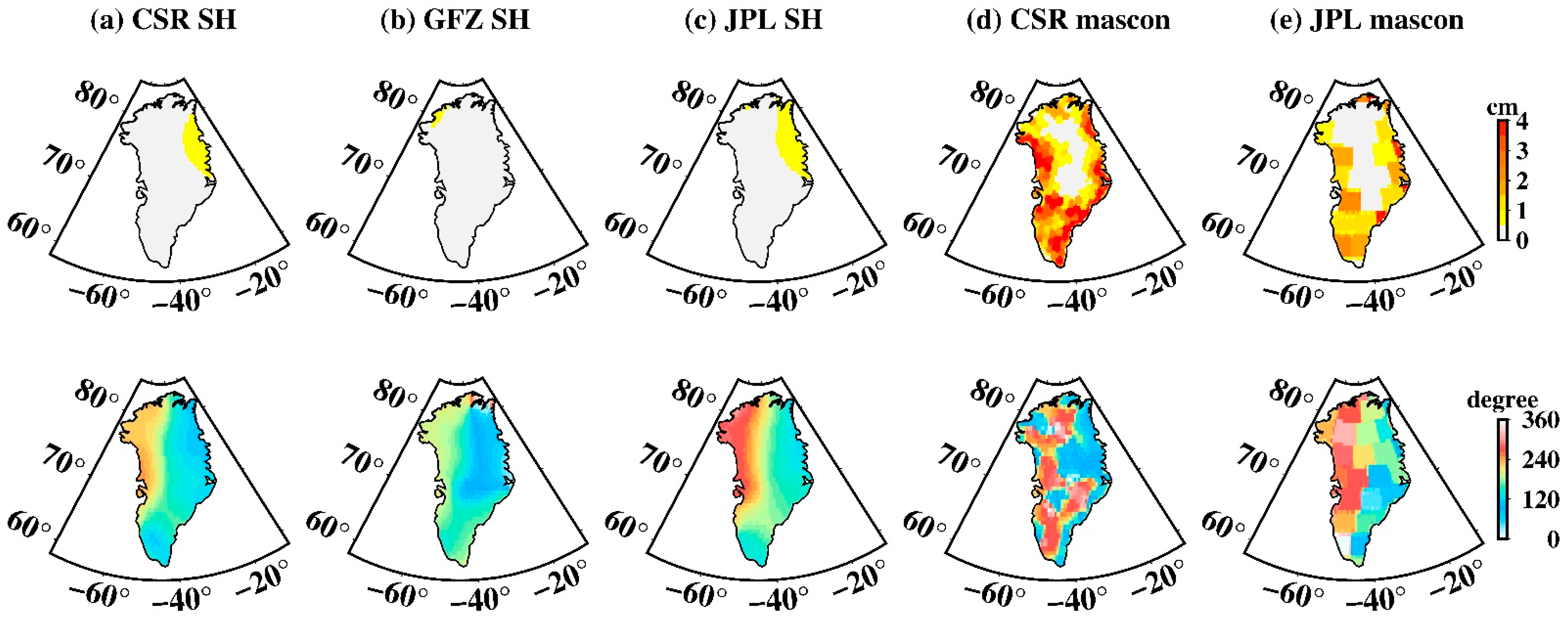
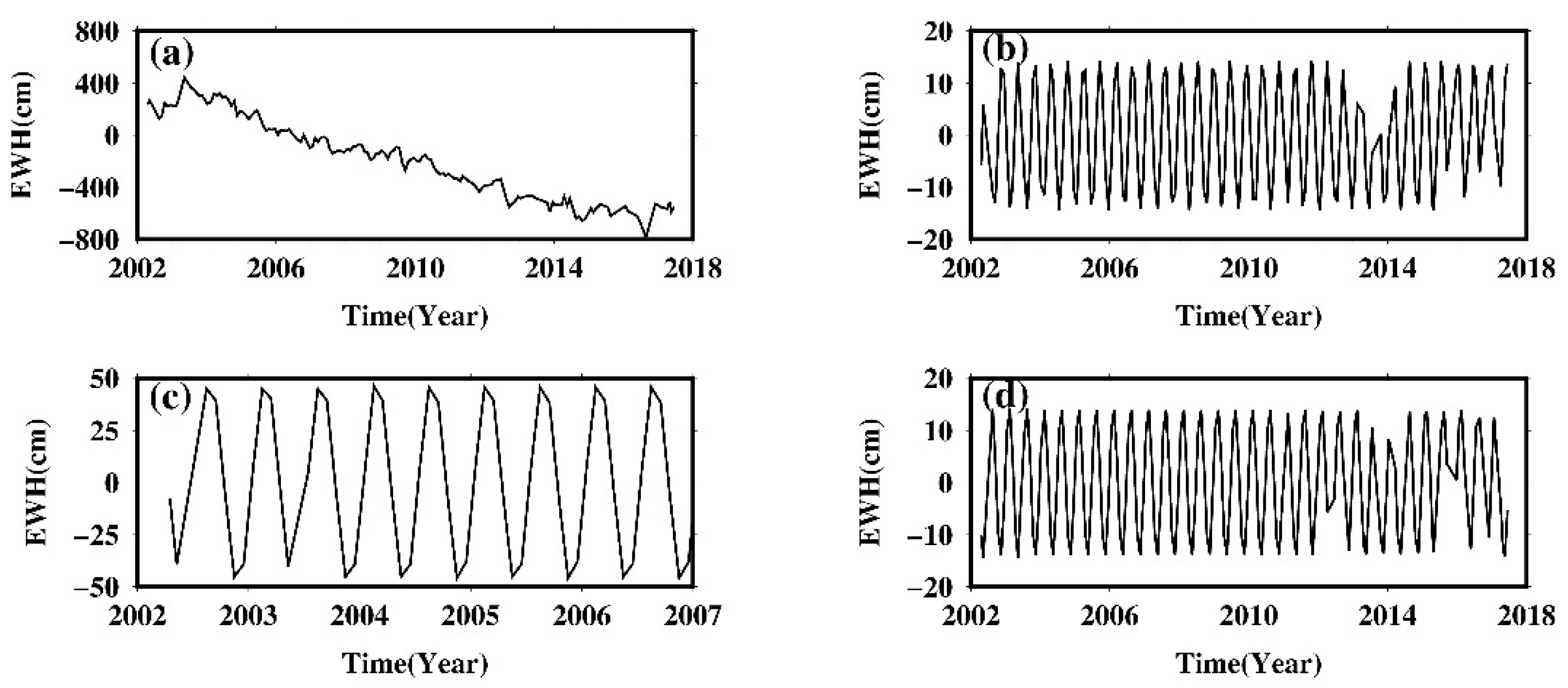
3.4. Tide Aliasing over Greenland

The amplitudes of S₂ tide aliasing in SH data over Greenland (Figure 9a–c) are less than 1.5 cm and are concentrated on the high latitudes of North Greenland, which is significantly better than those of West Antarctica. However, unexpected larger amplitudes over Greenland also appear in mascon data (Figure 9d,e), the largest amplitude of the CSR mascon is ~16.6 cm, and ~12.1 cm for the JPL mascon, almost 10 times larger in contrast with SH data. Confusingly, S₂ tide aliasing over Greenland in mascon data has completely different spatial distribution to that of SH data, even though the same tidal model is adopted. For mascon data, South Greenland, especially Southeast Greenland is more likely to be disturbed by S₂ tide aliasing.

P₁ aliasing is also pronounced over Greenland (Figure 10). For SH data the maximum amplitude is ~3 cm, spatially distributed mainly in South Greenland. Mascon data also shows a large P₁ amplitude, especially for the CSR mascon with the maximum amplitude of ~14.4 cm, compared with ~9.5 cm for that of the JPL mascon. The S₁ tide aliasing over Greenland is hardly noticeable for both the SH and mascon data (Figure 11), significantly better than S₂ and P₁, which can be neglected. All tide-aliasing errors over Greenland do not show notable propagation, as judged from their corresponding phase maps.

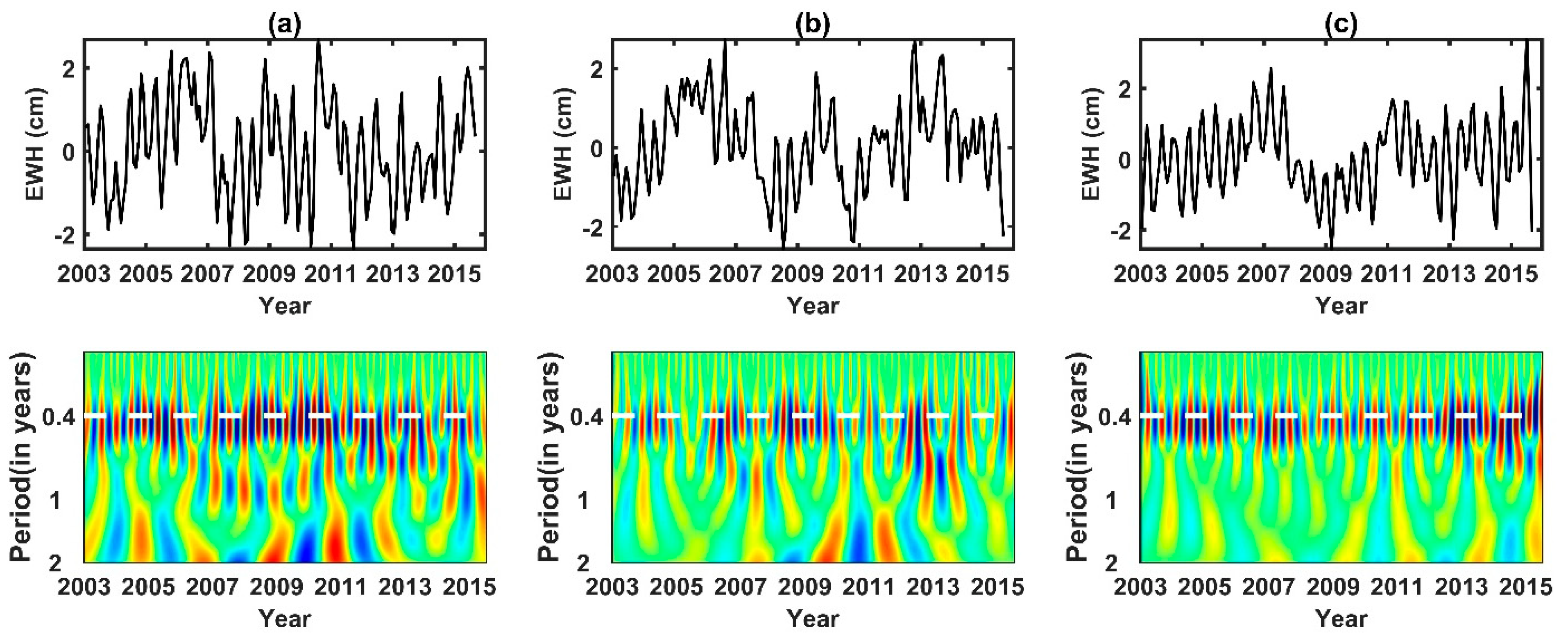
3.5. Comparison with Actual Seasonal Oscillation

The 161.0-day S₂ tide aliasing and the 171.2-day P₁ tide aliasing share similar periodicity with the semi-annual oscillation, while the 322.1-day S₁ tide aliasing has similar periodicity with the annual oscillation. This could lead to potential error in estimation of the seasonality. For example, one needs at least 9 years observation to separate the P₁ aliasing and semi-annual oscillation, otherwise, the so-called “semi-annual oscillation” fitted by least-square, actually involves aliasing error. Figure 12 shows the impact of P₁ aliasing on the estimation of semi-annual oscillation at a selected point A in Figure 10, with the most significant P₁ amplitude over Greenland. When the length of data is less than 9 years (e.g., 2002–2017; Figure 12c), the fitted “semi-annual” has a larger amplitude (~50 cm) than it actually is (~15 cm, which is fitted from Figure 12a for the period 2002–2017; see Figure 12d). The “semi-annual” oscillation in Figure 12c combines the actual semi-annual variation and the P₁ aliasing (Figure 12b). There is a similar situation for S₂—when the data length is shorter than 4 years, the S₂ aliasing will also have significant impact on the estimation of semi-annual oscillation.

Figure 13 shows the amplitudes of Antarctica’s and Greenland’s semi-annual oscillation. For regions over West Antarctica, the S₂ tide aliasing (Figure 3) is troublesome because it has much larger amplitude than the semi-annual oscillation, while P₁ (Figure 7) has limited effect on it. For Greenland, both S₂ (Figure 9) and P₁ (Figure 10) aliasing could lead to potential mistakes in estimation of the semi-annual variation, particularly for Southeast Greenland. Compared with semi-annual oscillation, the annual oscillation is the dominant component of Antarctica seasonal variations; as shown in Figure 14, its amplitude by far outweighs that of the S₁ aliasing, showing that S₁ has a limited effect on the annual oscillation, both for Antarctica and Greenland.

4. Discussion

We show several aliasing errors in current GRACE gravity field solutions that are worth noticing—particularly of the 161.0-day S₂ tide aliasing which is mainly located in West Antarctica. However, the 161.0-day period is probably not the only S₂ problem. Any number of errors can show up at the 161.0-day period when the orbit plane aligns with the sun. So radiational drag effects and heating problems (leading to accelerometer problems) can appear at this period. The 161.0-day period also appears in GRACE low-zonal Stokes coefficients, particularly C₂₀ and C₄₀ [13]. After analysis of the of the cross-track component of the GRACE accelerometer data, Cheng and Ries [25] suggested a temperature-dependent systematic error in the accelerometer data could be a cause. They concluded that the anomalous signal in C₂₀ zonal coefficients cannot be attributed to aliasing from the errors in the S₂ tide. They were looking only at C₂₀, but much of the argument applies to other zonal terms. Thus in the present work, other GRACE low zonal coefficients, e.g., C₃₀, C₄₀, and C₅₀, were also investigated. Figure 15 shows the time series of the fitted 161.0-day sinusoids in GRACE low zonal coefficients C₃₀, C₄₀, and C₅₀. Because C₂₀ used in this work has been replaced by SLR observation, no extra consideration is required. The amplitudes of the 161.0-day temperature-dependent systematic error in GRACE low zonal coefficients are quite small, just about 1% of the signal itself—greatly improved on those of the previous RL04 version (cf. Chen et al. [13]).

In order to quantify the contribution of the temperature-dependent error to the global amplitude of the 161.0-day period, we first removed the fitted 161.0-day sinusoids in those above-mentioned zonal coefficients, then re-fitted the amplitude of the 161.0-day period in the GRACE data, as shown in Figure 16. There was no obvious difference between Figure 16 and Figure 2 (as expected). S₂ in high latitudes, tropical oceans, and the Amazon River basin were still pronounced, suggesting that the errors of tidal models mostly account for the 161.0-day signal in GRACE data. In other words, temperature-caused error cannot be the major contributor in accounting for the 161.0-day oscillation in GRACE data.

A puzzling phenomenon is why mascon solutions show such significant larger aliasing error than SH solutions, even though they use the same tidal models. For example, in contrast to the traditional unconstrained SH solutions, the CSR mascon solutions inverse surface-mass changes by a two-step regularization matrix [22]. The first regularization matrix aims to suppress the signal leakage of the land signals into the ocean, and generates an intermediate solution have little or no leakage. The intermediate solution is then further optimized by the second regularization matrix; meanwhile, the stripe error in GRACE data is also greatly reduced. It seems that mason solutions mistake the tide aliasing as the leakage signal of the land ice-mass into oceans, and have unintentionally amplified the aliasing error by the first regularization matrix. The convincing evidence is that, almost without exception, those above-mentioned aliasing errors all mainly concentrate on the coastal regions. The stripe-like aliasing over the tropical oceans might be recognized as the stripe error in GRACE data, and is suppressed by the second regularization matrix. This is consistent with the significant reduced tide aliasing over the tropical ocean in mascon solutions.

5. Conclusions

In the present work, we investigated the S₂, P₁, and S₁ tide-aliasing error in the latest GRACE RL06 product, for both SH and mascon data. Several facts found during the studied period are worth noting:

(i)

Tide aliasing is still a major error of current GRACE RL06 observations, particularly for high latitudes where tide observation is lacking.

(ii)

S₂ aliasing is more pronounced over West Antarctica, while the P₁ aliasing shows the strongest amplitude over South Greenland. Moreover, S₂ aliasing over Antarctica is clearly an eastward circumpolar wave that completes a full clockwise circuit around Antarctica in about two years.

(iii)

Mascon data shows an incredibly large tide-aliasing error in comparison to SH data. The mascon solutions might have unintentionally “amplified” the tidal aliasing error on land due to the regularization (or constraint) applied for reducing land and ocean leakage.

(iv)

S₂ and P₁ aliasing can cause a potential obstacle on glacier’s semi-annual signal estimation in parts of the polar regions, due to the fact that they share similar periodicity.

Although certain tide-aliasing errors are evidently identified in this paper, unless the tidal models are improved, they will continue to exist in GRACE observations. We strongly recommend that the aliasing error should be fully considered when using GRACE for studying glacier variations at high latitudes, especially for mascon data.

References

1. Tapley, B.D.; Bettadpur, S.; Watkins, M.M.; Reigber, C. The gravity recovery and climate experiment; mission overview and early results. Geophys. Res. Lett. 2004, 31, L09607. [Google Scholar] [CrossRef] [Green Version]
2. Han, S.C.; Jekeli, C.; Shum, C.K. Time-variable aliasing effects of ocean tides, atmosphere, and continental water mass on monthly mean GRACE gravity field. J. Geophys. Res. 2004, 109, B04403. [Google Scholar] [CrossRef]
3. Tapley, B.D.; Watkins, M.M.; Flechtner, F.; Reigber, C.; Bettadpur, S.; Rodell, M.; Sasgen, I.; Famiglietti, J.S.; Landerer, F.W.; Chambers, D.P.; et al. Contributions of GRACE to understanding climate change. Nat. Clim. Chang. 2019, 9, 358–369. [Google Scholar] [CrossRef] [PubMed]
4. Velicogna, I.; Wahr, J.; Dool, H.V.D. Can surface pressure be used to remove atmospheric contributions from GRACE data with sufficient accuracy to recover hydrological signals? J. Geophys. Res. 2001, 106, 16415–16434. [Google Scholar] [CrossRef]
5. Nyquist, H. Certain topics in telegraph transmission theory. Trans. AIEE 1928, 47, 617–644. [Google Scholar] [CrossRef]
6. Liu, W.; Sneeuw, N. Aliasing of ocean tides in satellite gravimetry: A two-step mechanism. J. Geod. 2021, 95, 134. [Google Scholar] [CrossRef]
7. Dobslaw, H.; Wolf, I.B.; Dill, R.; Poropat, L.; Thomas, M.; Dahle, C.; Esselbom, S.; Konig, R.; Flechtner, F. A new high-resolution model of non-tidal atmosphere and ocean mass variability for de-aliasing of satellite gravity observations: AOD1B RL06. Geophys. J. Int. 2017, 211, 263–269. [Google Scholar] [CrossRef] [Green Version]
8. Knudsen, P. Ocean tides in GRACE monthly averaged gravity fields. Space Sci. Rev. 2003, 108, 261–270. [Google Scholar] [CrossRef]
9. Ray, R.D.; Rowlands, D.D.; Egbert, G.D. Tidal models in a new era of satellite gravimetry. Space Sci. Rev. 2003, 108, 271–282. [Google Scholar] [CrossRef]
10. Ray, R.D.; Luthcke, S.B. Tide model errors and GRACE gravimetry: Towards a more realistic assessment. Geophys. J. Int. 2006, 167, 1055–1059. [Google Scholar] [CrossRef]
11. Knudsen, P.; Andersen, O.; Khan, S.A.; Høyer, J.L. Ocean tide effects on GRACE gravimetry. Int. Assoc. Geod. Symp. 2001, 123, 159–164. [Google Scholar] [CrossRef]
12. Han, S.C.; Shum, C.K.; Matsumoto, K. GRACE observations of M2 and S2 ocean tides underneath the Filchner-Ronne and Larsen ice shelves, Antarctica. Geophys. Res. Lett. 2005, 32, L20311. [Google Scholar] [CrossRef]
13. Chen, J.L.; Wilson, C.R.; Seo, K.W. S2 tide aliasing in GRACE time-variable gravity solutions. J. Geod. 2009, 83, 679–687. [Google Scholar] [CrossRef]
14. Seo, K.W.; Wilson, C.R.; Han, S.C.; Waliser, D.E. Gravity recovery and climate experiment (GRACE) alias error from ocean tides. J. Geophys. Res. 2008, 113, B03405. [Google Scholar] [CrossRef] [Green Version]
15. Cartwright, D.E.; Tayler, R.J. New computations of the tide-generating potential, Geophys. J. Roy. Astron. Soc. 1971, 33, 253–264. [Google Scholar] [CrossRef] [Green Version]
16. Moore, P.; King, M. Antarctic ice mass balance estimates from GRACE: Tidal aliasing effects. J. Geophys. Res. 2008, 113, F02005. [Google Scholar] [CrossRef] [Green Version]
17. Swenson, S.; Chambers, D.; Wahr, J. Estimating geocenter variations from a combination of GRACE and ocean model output. J. Geophys. Res. 2008, 113, B08410. [Google Scholar] [CrossRef] [Green Version]
18. Loomis, B.D.; Rachlin, K.E.; Luthcke, S.B. Improved Earth oblateness rate reveals increased ice sheet losses and mass-driven sea level rise. Geophys. Res. Lett. 2019, 46, 6910–6917. [Google Scholar] [CrossRef]
19. Peltier, W.R.; Argus, D.F.; Drummond, R. Comment on “An assessment of ICE-6G_C (VM5a) glacial isostatic adjustment model” by Purcell et al. J. Geophys. Res. 2018, 123, 2019–2028. [Google Scholar] [CrossRef]
20. Li, Z.; Zhang, Z.Z.; Scanlon, B.R.; Sun, A.Y.; Pan, Y.; Qiao, S.Q.; Wang, H.S.; Jia, Q.Y. Combining GRACE and satellite altimetry data to detect change in sediment load to the Bohai Sea. Sci. Total Environ. 2022, 818, 151677. [Google Scholar] [CrossRef]
21. Chen, J.L.; Wilson, C.R.; Blankship, D.; Tapley, B.D. Accelerated Antarctic ice loss from satellite gravity measurements. Nat. Geosci. 2009, 2, 859–862. [Google Scholar] [CrossRef]
22. Save, H.; Bettadpur, S.; Tapley, B.D. High-resolution CSR GRACE RL05 mascons. J. Geophys. Res. 2016, 120, 2648–2671. [Google Scholar] [CrossRef]
23. Watkins, M.M.; Wiese, D.M.; Yuan, D.; Boening, C.; Landerer, F.W. Improved methods for observing Earth’s time variable mass distribution with GRACE using spherical cap mascons. J. Geophys. Res. 2015, 120, 2648–2671. [Google Scholar] [CrossRef]
24. Chao, B.F. Caveats on the equivalent-water-thickness and surface mascon solutions derived from the GRACE satellite-observed time-variable gravity. J. Geod. 2016, 90, 807–813. [Google Scholar] [CrossRef]
25. Cheng, M.K.; Ries, J. The unexpected signal in GRACE estimates of C20. J. Geod. 2017, 91, 897–914. [Google Scholar] [CrossRef]
26. Kaula, W. Theory of Satellite Geodesy; Blaisdell: Waltham, MA, USA, 1996. [Google Scholar]
27. Deng, X.; Featherstone, W.E. A coastal retracking system for satellite radar altimeter waveforms: Application to ERS-2 around Australia. J. Geophys. Res. 2006, 111, C06012. [Google Scholar] [CrossRef] [Green Version]
28. Bettadpur, S. CSR Level-2 Processing Standards Document for Product Release 04, GRACE 327-742, The GRACE Project, Center for Space Research, University of Texas at Austin. 2007. Available online: ftp://isdcftp.gfz-potsdam.de/grace/DOCUMENTS/Level-2/ (accessed on 25 October 2022).
29. Kvas, A.; Behzadpour, S.; Ellmer, M.; Klinger, B.; Strasser, S.; Zehentner, N.; Mayer-Gürr, T. ITSG-Grace2018: Overview and evaluation of a new GRACE-only gravity field time series. J. Geophys. Res 2019, 124, 9332–9344. [Google Scholar] [CrossRef] [Green Version]
30. Preisendorfer, R.W. Principal Component Analysis in Meteorology and Oceanography; Elsevier: New York, NY, USA, 1988. [Google Scholar]
31. Li, Z.; Chao, B.F.; Zhang, Z.Z.; Jiang, L.M.; Wang, H.S. Greenland interannual ice mass variations detected by GRACE time-variable gravity. Geophys. Res. Lett. 2022, 49, e2022GL100551. [Google Scholar] [CrossRef]
32. Li, Z.; Chao, B.F.; Wang, H.S.; Zhang, Z.Z. Antarctica ice-mass variations on interannual timescale: Coastal Dipole and propagating transports. Earth Planet. Sci. Lett. 2022, 595, 117789. [Google Scholar] [CrossRef]
Figure 1. Time series of the non-secular, non-seasonal GRACE low Stokes coefficients and their conventional discrete Fourier spectrum. (a1,a3,a5) C21 time series from CSR, GFZ, and JPL, respectively, and (a2,a4,a6) are their corresponding Fourier spectra; (b1b6) C21 time series from CSR, GFZ, and JPL, respectively, and (a1a6) are their corresponding Fourier spectra for S21; (c1c6) C21 time series from CSR, GFZ, and JPL, respectively, and (a1a6) are their corresponding Fourier spectra for C22; (d1d6) C21 time series from CSR, GFZ, and JPL, respectively, and (a1a6) are their corresponding Fourier spectra for S22.
Remotesensing 14 05403 g001
Figure 2. Least-square fit of the global amplitudes of S2, P1, and S1 tide aliasing. (ae) Amplitude maps of the S2 aliasing in CSR SH data, GFZ SH data, JPL SH data, CSR mascon data, and JPL mascon data, respectively; (f,g) amplitude maps of the S2 aliasing in CSR SH data, GFZ SH data, JPL SH data, CSR mascon data, and JPL mascon data, respectively; (ho) amplitude maps of the S1 aliasing in CSR SH data, GFZ SH data, JPL SH data, CSR mascon data, and JPL mascon data, respectively.
Remotesensing 14 05403 g002
Figure 3. Spatial amplitude and the corresponding phase maps of S2 tide aliasing over Antarctica. (ae) Estimated from CSR SH data, GFZ SH data, JPL SH data, CSR mascon data, and JPL mascon data, respectively. The upper row is the spatial amplitude and the bottom row is their corresponding phase.
Remotesensing 14 05403 g003
Figure 4. EOF-mode solutions (spatial patter and time series) of the (non-seasonal) mass variation over Antarctica from GRACE data. (ad) Modes 1-4 (Mode 1 representing ACD). The spatial patterns are normalized with respect to standard deviation; the time series manifests equivalent water-thickness in cm.
Remotesensing 14 05403 g004
Figure 5. Time-frequency wavelet spectra of EOF Modes 2–4 (from Figure 4). Prominent signals at the quasi-periodicity of ~0.4 year or ~161.0 days are evident. (ac) time series of EOF Mode 2–4 (Upper panels) and corresponding wavelet spectra (lower panels).
Remotesensing 14 05403 g005
Figure 6. The leading CEOF mode of the non-seasonal mass variation over Antarctica from GRACE data (after removal of the EOF Mode 1 or ACD). For amplitude: (a) root-mean-square amplitude map; (b) corresponding strength variation. For phase: (c) spatial phase map in degree (largely clockwise spin or eastward propagation); (d) unwrapped temporal phase.
Remotesensing 14 05403 g006
Figure 7. P1 tide aliasing over Antarctica. (ae) Spatial amplitude and the corresponding phase maps estimated from CSR SH data, GFZ SH data, JPL SH data, CSR mascon data, and JPL mascon data, respectively.
Remotesensing 14 05403 g007
Figure 8. S1 tide aliasing over Antarctica. (ae) Spatial amplitude and the corresponding phase maps estimated from CSR SH data, GFZ SH data, JPL SH data, CSR mascon data, and JPL mascon data, respectively.
Remotesensing 14 05403 g008
Figure 9. Spatial amplitude and the corresponding phase maps of S2 tide aliasing over Greenland. (ae) Estimated from CSR SH data, GFZ SH data, JPL SH data, CSR mascon data, and JPL mascon data, respectively. The upper row is the spatial amplitude and the bottom row is their corresponding phase.
Remotesensing 14 05403 g009
Figure 10. Spatial amplitude and the corresponding phase maps of P1 tide aliasing over Greenland. (ae) Estimated from CSR SH data, GFZ SH data, JPL SH data, CSR mascon data, and JPL mascon data, respectively. The upper row is the spatial amplitude and the bottom row is their corresponding phase.
Remotesensing 14 05403 g010
Figure 11. Spatial amplitude and the corresponding phase maps of S1 tide aliasing over Greenland. (ae) Estimated from CSR SH data, GFZ SH data, JPL SH data, CSR mascon data, and JPL mascon data, respectively. The upper row is the spatial amplitude and the bottom row is their corresponding phase.
Remotesensing 14 05403 g011
Figure 12. (a) Time series of point A at Figure 10 from CSR mascon data; (b) the fitted 171.2-day P1 sinusoid; (c) least-square fits of the simi-annual oscillation for the period 2002–2006; (d) least-square fits of the simi-annual oscillation for the period 2002–2017.
Remotesensing 14 05403 g012
Figure 13. Spatial amplitude maps of semi-annual oscillation over Antarctica and Greenland. (ae) Estimated from CSR SH data, GFZ SH data, JPL SH data, CSR mascon data, and JPL mascon data, respectively.
Remotesensing 14 05403 g013
Figure 14. Annual oscillation over Antarctica and Greenland. (a) CSR SH data, (b) CSR mascon data, (c) JPL mascon data, (d) CSR mascon data, (e) JPL mascon data.
Remotesensing 14 05403 g014
Figure 15. (a,c,e) Time series of GRACE low zonal coefficients C30, C40, and C50, respectively; (b,d,f) the fitted S2 aliasing series from C30, C40, and C50, respectively.
Remotesensing 14 05403 g015
Figure 16. Global amplitude maps of S2 tide aliasing after removal of the 161.0-day oscillation in low zonal coefficients. (a) Fitted from CSR SH data; (b) fitted from GFZ SH data; (c) fitted from JPL SH data.
Remotesensing 14 05403 g016