Abstract
Using unmanned aerial vehicle (UAV) hyperspectral images to accurately estimate the chlorophyll content of summer maize is of great significance for crop growth monitoring, fertilizer management, and the development of precision agriculture. Hyperspectral imaging data, analytical spectral devices (ASD) data, and SPAD values of summer maize in different key growth periods were obtained under the conditions of a micro-spray strip drip irrigation water supply. The hyperspectral data were preprocessed by spectral transformation methods. Then, several algorithms including Findpeaks (FD), competitive adaptive reweighted sampling (CARS), successive projections algorithm (SPA), and CARS_SPA were used to extract the sensitive characteristic bands related to SPAD values from the hyperspectral image data obtained by UAV. Subsequently, four machine learning regression models including partial least squares regression (PLSR), random forest (RF), extreme gradient boosting (XGBoost), and deep neural network (DNN) were used to establish SPAD value estimation models. The results showed that the correlation coefficient between the ASD and UAV hyperspectral data was greater than 0.96 indicating that UAV hyperspectral image data could be used to estimate maize growth information. The characteristic bands selected by different algorithms were slightly different. The CARS_SPA algorithm could effectively extract sensitive hyperspectral characteristics. This algorithm not only greatly reduced the number of hyperspectral characteristics but also improved the multiple collinearity problem. The low frequency information of SSR in spectral transformation could significantly improve the spectral estimation ability for SPAD values of summer maize. In the accuracy verification of PLSR, RF, XGBoost, and the DNN inversion model based on SSR and CARS_SPA, the determination coefficients (R2) were 0.81, 0.42, 0.65, and 0.82, respectively. The inversion accuracy based on the DNN model was better than the other models. Compared with high-frequency information, low-frequency information (DNN model based on SSR and CARS_SPA) had a strong estimating ability for SPAD values in summer maize canopy. This study provides a reference and technical support for the rapid non-destructive testing of summer maize.
1. Introduction
Chlorophyll is one of the important physiological and biochemical parameters of plants. Its content can reflect the photosynthetic capacity, nitrogen absorption and utilization, and nutritional growth status of plants. The rapid and accurate estimation of crop chlorophyll content plays an important role in crop growth monitoring and real-time precision agriculture [1,2]. The chlorophyll content in crop leaves can be obtained quickly and in a non-destructive manner using SPAD-502. However, this method is based on the rapid detection of chlorophyll in leaves, which is time-consuming and laborious because it requires measuring different leaves repeatedly. This also applies to the area measurement method, which is unable to achieve large-scale accurate measurements in time and space and thus cannot meet the requirements for the monitoring of modern agriculture practices. Therefore, there is an urgent need to develop a rapid monitoring method that can reflect the SPAD values of the crop canopy at the field scale [3,4,5].
With the development of remote sensing technologies, UAV remote sensing technology has become an important means of agricultural monitoring due to its flexibility, comprehensiveness, wide coverage, and high spatial–temporal resolution [6,7,8]. Many studies have shown that the use of UAVs to acquire spectral images, combined with existing mature algorithms, can be used to effectively monitor SPAD values. UAV images can be divided into multispectral and hyperspectral images. Multispectral images have a high spatial resolution and are easy to operate. The wide-band extracted from them, combined with the existing spectral index, can be used to quickly and non-destructively monitor the SPAD value of crops [9]. In recent years, it has been found that the estimation model established for the existing wide-band spectrum index is vulnerable to the interference of environmental factors such as noise and soil. When monitoring other crops, the estimation model has shown poor robustness and a reduced model accuracy. The interference from external environmental factors can be reduced by optimizing the corresponding frequency band to construct a new spectral index. For multispectral images, although they are easy to obtain and process, the disadvantage is that the amount of spectral information is small, and the frequency band is wide. As a result, it is impossible to optimize the width between bars, which affects the robustness and accuracy of models used to estimate different crops, thus hindering large-area accurate estimation [10].
Compared with multispectral images, hyperspectral images have the characteristics and advantages of the “spectral-image cube”. While obtaining two-dimensional centimeter-level spatial image information of the ground, it also obtains the continuous spectral information of ground objects with many narrow bands and a band width of less than 5 nm. In recent years, research using UAV hyperspectral technology has focused on the detection of chlorophyll content in the canopy leaves of field crops. In previous studies, the chlorophyll in maize and other crops has been mostly estimated using the spectral band combination vegetation index method, which can be roughly divided into a combination of a single vegetation index and a multi vegetation index. Other studies have used the single band or full band information of crop leaves. The use of a single sensitive band for modeling may lead to the loss of effective information, thereby greatly reducing the accuracy of the model. However, when full-wave band modeling is used, the accuracy of the model will also be affected due to a large amount of redundant information in the spectrum. Therefore, analyzing the spectral characteristics of maize chlorophyll to determine its sensitive band is the first condition to improve the efficiency of the model’s operation, simplify the model’s structure, and enhance the stability of the model. Many studies have been conducted in the same planting environment and single growth period over a long timescale without considering whether the planting environment and growth period will affect the accuracy of the estimation model. The remote sensing monitoring of chlorophyll using a UAV platform and a hyperspectral camera has been widely used in maize and wheat, among other crops [11,12,13].
In recent years, machine learning algorithms, such as deep learning, have been applied to the fields of land type classification, agricultural status, and disaster monitoring [14,15,16,17]. In their study of the UAV spectrum, Guo et al. [18] used vegetation indices (VIs), RF and support vector machines (SVM) to build a summer maize SPAD values estimation model. In this study, the extracted spectral parameters were combined with the algorithm to build a physiological parameter inversion model. In recent years, band dimensionality reduction algorithms, such as successive projections algorithm (SPA) [19], variable projection importance (VIP) [20], and principal component analysis (PCA) [21], have been widely used in the field of ground monitoring and satellite remote sensing [22,23]. These feature-band-selection algorithms can effectively remove the redundancy in high-dimensional data, thereby reducing the risk of overfitting the inversion model, enabling the building of a robust model with a high prediction accuracy [24,25]. However, few studies have reported on the estimation of the SPAD values of summer maize based on the combination of a feature-band-selection algorithm with machine learning using UAV hyperspectral data.
In this study, the SPAD values of each key growth period of summer maize and the related UAV hyperspectral data were obtained. After spectral transformation from the original hyperspectral image, the feature bands sensitive to the SPAD values were extracted using a feature extraction algorithm. Then, four regression model methods (partial least squares regression (PLSR), random forest (RF), extreme gradient boosting (XGBoost), and deep neural network (DNN)) were used to construct the inversion model of SPAD values for summer maize based on the selected characteristic bands. Finally, the estimation results of four machine learning models were compared and analyzed, and the optimal model for estimating the SPAD values of summer maize was selected. These findings provide a technical basis for the estimation of the phenotypic indicators of various crops in key growth periods.
2. Materials and Methods
2.1. Study Sites and Experimental Design
The summer maize experiment was conducted in the Hohhot agricultural research demonstration base (40°26′0.29″N, 109°36′25.99″E), a dry agricultural region in China. The southern region of this site is hilly, while the northern region is an alluvial plain with an average altitude of 1000 m. The annual average sunshine duration in this area is approximately 3000 h. The air is dry, and the climate is a temperate continental climate. The precipitation levels are low across the four seasons, with an average annual precipitation of 320 mm. The crops commonly grown in this region are maize and sunflowers, which are planted once a year.
The variety of summer maize planted in 2021 was Junkai 918, which is characterized by drought resistance and wind and sand resistance. It is widely planted in Inner Mongolia. The planting row direction was east–west, with row spacing of 55 cm and plant spacing of 24 cm. The sowing time was 6 May, the emergence time was 12 May, the heading time was 21 July, and the harvesting time was September 11. Since the precipitation levels in the experimental area are very low, it is difficult to meet the needs of largescale crop planting. To address this, in this study, micro-drip irrigation was used as the main irrigation equipment for summer maize. However, the technology used for micro-spray strip drip irrigation is not advanced. In particular, this type of irrigation method lacks effective maintenance and repair methods, which leads to the aging of the equipment due to daily use. As a result, some areas of the experimental area could not be irrigated properly, reducing the overall irrigation efficiency and imposing significant constraints on the development of the maize. As shown in Figure 1, the planting area of crops in the test area was 1.25 hm2. The soil in the experimental area comprised sand (0.03~1.9 mm), silt (0.003~0.05 mm), and clay (<0.003 mm), accounting for 81.7%, 11.6%, and 6.7% of the soil, respectively. The nitrogen, organic matter, phosphorus, and potassium contents were 17.24 mg/kg, 48.20 g/kg, 1.131 mg/kg, and 18.32 mg/kg, respectively. The field effective volumetric water capacity was 29%.
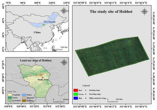
Figure 1.
Location of the study sites.
2.2. Data Collection
All experimental data, including hyperspectral imaging data based on UAV, the reflectivity of the handheld ASD spectrometer, and the SPAD values were collected in 2021 three consecutive times during the key growth stage of summer maize: 30 July (jointing stage), 12 August (tasseling stage), and 28 August (milky maturity stage).
2.2.1. UAV Hyperspectral Image Data Acquisition
The UAV platform consisted of a DJI M300rtk multi-rotor UAV (DaJiang Company, Shenzhen, China) and a Cubert S185 hyperspectral imager (Cubert GmbH, Ulm, Germany) using the parameters listed in Table 1. The 138 spectral bands of the S185 ranged from 450~998 nm visible light to near-infrared light. The spectral resolution of the hyperspectral data was 8 nm, while the sampling interval was 4 nm. The data obtained by the S185 hyperspectral imager included hyperspectral cube images (.cube format) and panchromatic images (.jpg format) with a high spatial resolution. UAV remote sensing acquisition was performed on a cloudless and windless day. Before hyperspectral data acquisition, the S185 was calibrated using a reference white board (Figure 2a). The flight altitude, flight speed, heading overlap, and lateral overlap of the UAV were set to 50 m, 5 m/s, 85%, and 75%, respectively. The data processing and overall technical route are shown in Figure 3.

Table 1.
Characterization of Cubert S185 device.
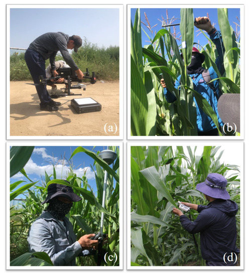
Figure 2.
(a) Cubert S185 hyperspectral white board calibration; (b) ASD high spectrometer; (c) RTK mobile station to determine SPAD observation position; (d) SPAD measurement.
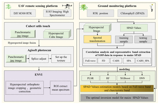
Figure 3.
Flow chart of summer maize SPAD values estimation model.
The ground hyperspectral data acquisition and UAV aerial survey were conducted simultaneously. A FieldSpec Handheld 2 handheld ground object spectrometer from the ASD Company of the United States was used with a spectrum acquisition range of 325~1075 nm and wavelength interval of 1 nm. In this study, five points were collected for each leaf, five spectra were recorded at each sampling point, and the mean value was taken as the final spectral curve of the leaf. On 30 July, the spectral data of five leaves were collected, and 25 spectral curves were accumulated (Figure 2b). In order to verify the validity of spectral information of the S185, the 325~450 nm blue violet light and 1000~1075 nm short-wave near-infrared bands that are prone to loud noise in the ASD spectrometer were cut off. The spectral range of 450–998 nm was reserved.
2.2.2. Measurement of SPAD Values
SPAD measurement is non-destructive to crops. The SPAD-502 Plus Portable Chlorophyll was used to determine the current relative amount of chlorophyll in the leaves by measuring the absorption rate of leaves in the red region and the near-infrared region. The result was a unit-free but highly repeatable measurement. Previous studies have used portable instruments (e.g., SPAD-502 Plus) to characterize SPAD with a satisfactory accuracy. The process of measuring the SPAD data using SPAD-502 Plus is shown in Figure 2d.
2.2.3. Data Analysis
A total of 30 samples were collected in each growth period, and a total of 90 SPAD values were collected, as shown in Figure 1. Real-time kinematic (RTK) sampling was used to locate and record the coordinates of each observation point (Figure 2c). Due to the errors caused by the equipment and its operation, 7 SPAD values were deleted, and the remaining 83 SPAD values were used for data analysis and model construction. To determine the robustness of the model to time changes, 51 samples were randomly selected from the total SPAD data as the training set and 32 samples as the validation set. The descriptive statistics of the SPAD values (unitless) of summer maize measured by the SPAD-502 Plus device are shown in Table 2.
Table 2.
Statistical summary of the in situ SPAD values of summer maize using a SPAD-502 Plus device.
The traditional spectral-data-processing method of mathematical transformation can be used to effectively enhance available information in the full-wave spectrum as well as compress unnecessary information by using mathematical methods to process and analyze smooth spectral reflectance (SSR) data. Among these methods, non-differential transformations, such as logarithmic spectral reflectance (LSR) and reciprocal spectral reflectance (RSR), help to highlight the low-frequency information in the spectrum, while differential transformations, such as differential spectral reflectance (DSR), logarithmic differential spectral reflectance (LDSR), and reciprocal differential spectral reflectance (RDSR), help to highlight the more subtle information in the spectrum. In particular, differential transformation is helpful for the coupling of varying frequency band information [26]. For remote sensing data with different spectral transformations, various algorithms, such as Findpeaks (FD) [27], SPA, competitive adaptive reweighted sampling (CARS) [28], and CARS_SPA [29], can be used to extract the sensitive characteristic bands of SPAD values in the hyperspectral stereo spatial data of UAV. Combined with full spectrum information, a SPAD value estimation model was constructed using four machine learning (ML) methods: PLSR, RF, XGBoost, and DNN. A technical diagram of the processing of the hyperspectral imaging data and data analysis for the summer maize SPAD values estimation model established by UAV remote sensing and ML is shown in Figure 3.
2.3. Algorithms for Wavelength Variable Selection
Four algorithms for wavelength variable selection were used in this study:
- (1)
- First, the FD function was used to automatically find the variance statistics (F). The peak value and the sensitive spectral band were determined. Then, the initial sensitive spectral features were extracted by using the position of the sensitive band [27], as shown in Equation (1):where x is the matrix composed of F, and band P is the F peak, l is the corresponding band position of the F peak, a is the minimum height of the F peak, and b is the minimum band distance between adjacent F peaks. The a of F of its spectral characteristics was set as 3.64, while b was set to 5.
- (2)
- SPA is a forward wavelength extraction method, which continuously circularly calculates the projection of one wavelength on the other unselected wavelengths to find the wavelength with the least amount of redundant information. This method can be used to reduce the collinearity of the input data group. A continuous projection algorithm can use a few columns of data extracted from the original data of all wavelengths, which can represent the vast majority of the information contained in the original data. Therefore, it is commonly used for the selection of the characteristic wavelength of a spectrum.
- (3)
- The CARS algorithm combines Monte Carlo sampling and the partial least squares (PLS) model regression coefficient to realize the selection of characteristic variables. To establish the PLS model, variables with a small weight of the absolute value of the regression coefficient in the PLS model are eliminated using reweighted sampling technology. Then, the PLS model is established based on residual variables to continue to eliminate. After multiple operations, the subset with the lowest root mean square error is selected as the characteristic wavelength through interactive verification. The PLS model was established using the CARS algorithm to screen the spectral data of each band and then compared with the full-wave band model. After screening the CARS variables, the root-mean-square error of cross-validation (RMSECV) and root-mean-square error of prediction (RMSEP) provided better results than full-wave band modeling, significantly improving the quality of the model.
- (4)
- The CARS_SPA algorithm combines the CARS and SPA algorithms, selects effective wavelengths, optimizes model fitting, and improves prediction performance. Specifically, CARS first obtains a set of potential characteristic bands related to the summer maize SPAD values. Secondly, based on the initial sensitive spectral features, the final sensitive spectral features are extracted by SPA. After the CARS and SPA variables are selected, the number of variables is reduced, and the model performance index is improved.
The wavelength variable selection methods of FD, CARS, SPA, and CARS_SPA were conducted in MATLAB R2018b (The MathWorks, Natick, MA, USA).
2.4. Modeling Methods
After the mathematical transformation of the hyperspectral images of the UAV, four regression methods (PLSR, RF, XGBoost, and DNN) were used to construct the estimation model of the SPAD values in the summer maize canopy. Among these, PLSR is a multivariate statistical data analysis method, which mainly involves the regression modeling of multiple dependent variables to various independent variables [30]. The PLSR method is more effective when the internal variables are highly linear. Moreover, the PLSR method can be used to address situations when the number of samples is less than the number of variables. PLSR analysis integrates the characteristics of principal component analysis (PCA), canonical correlation analysis, and linear regression analysis in the modeling process, thereby providing a more reasonable regression model. It is also able to better solve the multicollinearity problem, and is expressed as follows:
where is the input variable of the model, such as the spectral characteristic band, is the output variable (that is, the SPAD values of maize), is the dimension of the input variable (that is, the number of characteristic bands), is the number of samples, is the intercept, is the regression coefficient, is the deviation, and and are the latent variable and the corresponding coefficient, respectively.
Next, the RF algorithm is an ML algorithm for classification and prediction based on a bagging ensemble learning algorithm and a random space algorithm. RF algorithms are divided into RF classification and RF regression [12,31,32,33]. Compared with other ML algorithms, it has the following advantages: (i) a strong nonlinear simulation that can effectively deal with the problems associated with multivariable and large amounts of data. It does not need to delete variables and handle dimensions uniformly and can evaluate the importance of all variables at the same time; (ii) it has few parameters, a high operation efficiency, and a strong data mining ability; (iii) it is not prone to overfitting, has a high tolerance for outliers, missing values, and interference values, and has good robustness for data set feature mining.
XGBoost is an improved version of the algorithm of the gradient-boosting decision tree. In this algorithm, first- and second-order partial derivatives are used. Without selecting the specific form of the loss function, the leaf-splitting optimization calculation can be carried out by solely relying on the value of the input data. In essence, the selection of the loss function and the model algorithm are optimized. This decoupling increases the applicability of XGBoost, so that it selects the loss function as needed and adds a regular term to the loss function to control the complexity of the model, which is conducive to preventing overfitting, thereby improving the generalization ability of the model [34,35,36,37].
A neural network is a critical learning method in machine learning. It can be considered an algorithm obtained by abstracting the neuron structure from the point of view of information processing. It establishes a mathematical model for specific problems and divides it into different network structures according to different connection modes and algorithms. DNN is essentially an operation model comprising many neurons with specific operation rules and connections. In the neural network, each neuron will carry out a nonlinear transformation on the input signal through the activation function. In the connection relationship, the connection between every two neurons indicates that the passed data is weighted. The weight parameters can be seen from the memory of the artificial neural network for the data. In essence, the artificial neural network is often the fitting or logical expression of some algorithm function existing in nature [38].
The infrastructure of DNN is based on the traditional artificial neural network (ANN), which was first applied to recognizing handwritten characters in documents. Conventional artificial neural networks have three layers: input, hidden, and output. Generally, DNN has two to dozens of hidden layers, which makes the structure of DNN more complex, greatly improving its expression ability. Due to the many hidden layers, the training of DNN is typically complex. Therefore, DNN has many technical methods that differ from those of traditional artificial neural networks. For example, in terms of the loss function, the cross-entropy cost function is used to measure the gap between its model and learning samples.
For the establishment of the models, PLSR, RF and XGBoost were performed in scikit-learn 1.01 (Anaconda, Austin, TX, USA) using Python 3.6. The GridSearchcv method in sklearn was used to obtain the optimal kernel parameters of the RF and XGBoost models. The DNN model and cartographic were conducted in keras 2.4.3 and GDAL 3.0.2 (Anaconda, Austin, TX, USA). Finally, the optimal parameter model was used to retrieve the SPAD values of summer maize.
2.5. Evaluation of Model Performance for SPAD Value Modeling
The performance of the summer maize canopy SPAD values estimation model was evaluated using validation sample data. To objectively and comprehensively evaluate this estimation model, the determination coefficient (R2), the root-mean-square error (RMSE), mean absolute error (MAE) and mean relative error (MRE) were selected to comprehensively evaluate the SPAD values estimation model as shown in Formulas (3)–(6):
where is the measured SPAD values, is the average value of the measured SPAD values, the estimated value based on the SPAD values estimation model, is the average value of the estimated SPAD values, and is the total number of samples.
3. Results
3.1. Hyperspectral Imaging Data Processing and Verification of UAV Reliability
The hyperspectral images of the UAV collected at different periods of maize were spliced and synthesized using the Agisoft PhotoScan software (Agisoft Limited Liability Company (LLC), St. Petersburg, Russia). Image geometric correction, image clipping, and spectral transformation calculation were performed in the ENVI 5.6 software to identify the position of the sample points corresponding to the ground measurement in the summer maize test area and build a region of interest (ROI). The average spectral reflectance of the ground objects within the ROI range (2 × 2 pixel) was selected as the summer maize reflectance of the sample point to obtain the spectral reflectance data of each point. The display of the spectral transformation on 30 July is shown in Figure 4.
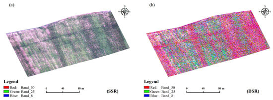
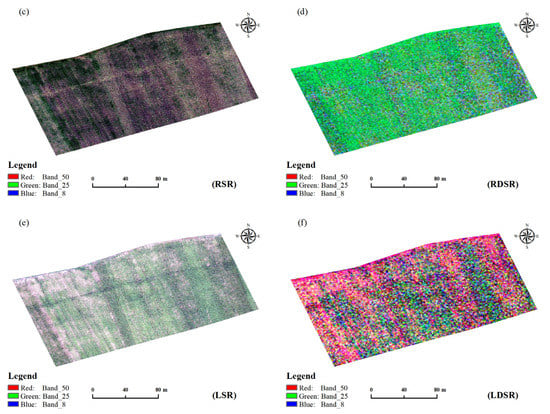
Figure 4.
Images of six spectral transformations of the original hyperspectral image of the UAV on 30 July: (a) SSR, (b) DSR, (c) RSR, (d) RDSR, (e) LSR, (f) LDSR.
To verify the reliability of the hyperspectral data collected by UAV, five groups of ASDs collected spectral data and the Cubert S185 hyperspectral data were used to calculate the spectral average reflectance of the two devices. The correlation analysis indicated that the smooth reflectance of the high spectrometer of Cubert S185 and ASD was highly consistent in the wavelength range of 454~838 nm, with overlaps in the green peak position and red edge region (Figure 5a). A large variation was observed in the band from 838 to 950 nm, which was possibly due to the boundary noise of the device within this band. The results of the Cubert S185 and ASD reflectance indicated that high-quality data were obtained, with an average R2 at different growth periods of 0.96 (Figure 5b).
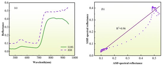
Figure 5.
Verification of the reliability of the Cubert S185 hyperspectral image data. (a) Comparison of spectral curves between ASD and Cubert S185. (b) Correlation analysis of spectral data between ASD and Cubert S185.
3.2. Characteristic Band Selection Associated with Maize SPAD Values
After the UAV full-wave images were preprocessed by dimension reduction, the selected characteristic bands of the different dimension reduction algorithms were found to be roughly the same. However, some differences were observed in the number and proportion of the selected bands, as shown in Figure 6. First, the wavelengths of 474, 562, 714, 806, 838, 886, and 930 nm in the SSR spectral images were selected, accounting for 5.07% of the total variables. In contrast, the spectral bands at 466, 490, 514, 546, 586, 618, 666, 690, 714, 77, 826, 870, 918, 958, and 990 nm in the DSR spectral images accounted for 10.87% of the total variables. The spectral bands at 458, 490, 562, 714, 838, 930, and 958 nm in the LSR spectral images accounted for 5.07% of the total variables. Finally, the spectral bands at 466, 490, 514, 546, 570, 606, 630, 658, 690, 758, 790, 826, 874, 918, 958, and 994 nm in the LDSR spectral images accounted for 11.59% of the total variables. The spectral bands at 458, 490, 562, 714, 838, 894, 930, and 962 nm in the RSR spectral images accounted for 5.79% of the total variables, while the spectral bands at 466, 490, 514, 56, 618, 658, 686, 758, 790, 826, 866, 918, and 958 nm in the RDSR spectral images accounted for 9.42% of the total variables.
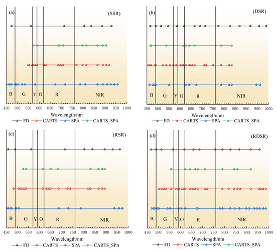
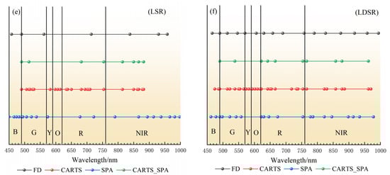
Figure 6.
Distribution of feature band selection of feature extraction algorithms for different spectral transformations: (a) SSR, (b) DSR, (c) RSR, (d) RDSR, (e) LSR, (f) LDSR.
The results from the bands where CARS was selected indicated that the wavelengths of 550, 554, 566, 574, 582, 590, 622, 630, 686, 694, 702, 710, 770, 798, 814, 866, 890, 906, and 918 nm in the SSR spectral images were selected by the CARS algorithm, accounting for 13.76% of the total variables. The spectral bands at 454, 462, 466, 470, 486, 490, 522, 538, 554, 570, 582, 602, 610, 614, 626, 642, 650, 654, 666, 710, 718, 750, 786, 822, and 834 nm in the DSR spectral images accounted for 18.11% of the total variables. In addition, hyperspectral characteristic bands extracted by the SPA algorithm were adopted, such as the spectral bands at 450, 462, 470, 474, 490, 498, 502, 522, 534, 582, 674, 718, 786, 810, 866, 890, 910, 926, 942, and 958 nm in the SSR spectral images, which accounted for 14.49% of the total variables. The spectral bands at 462, 478, 486, 490, 550, 626, 642, 674, 786, 822, 834, 946, and 962 nm in the DSR spectral images accounted for 9.42% of the total variables.
The number of characteristic bands selected by the initial CARS and SPA was large, which led to problems such as having a complex model, large calculation amount, and poor robustness. Then, the characteristic bands used for modeling were extracted using the CARS_SPA combined algorithm. The distribution of the characteristic bands corresponding to the CARS_SPA algorithm was as follows: (1) SSR: 574, 590, 686, 694, 710, 798, 814, 866, 890, and 906 nm. (2) DSR: 466, 470, 490, 538, 614, 626, 642, 666, 786, and 834. (3) RSR: 526, 538, 614, 650, 682, 830, 866, 882, and 894 nm. (4) RDSR: 558, 622, 642, 666, 678, 710, 790, 842, 858, and 918 nm. (5) LSR: 490, 514, 682, 754, 814, 850, 866, and 882 nm. (6) LDSR: 490, 538, 622, 642, 666, 754, 766, 858, 878, and 962 nm.
It can be seen that under the CARS_SPA algorithm, the absorption characteristics of chlorophyll (575 nm), the red edge characteristics of the crops (710 nm), and the strong reflection characteristics of the crop leaf tissues (814, 866, 890, and 906 nm) were well extracted from the SSR spectral characteristics. Obviously, the CARS_SPA algorithm could effectively extract the hyperspectral characteristic bands and greatly reduce the data redundancy of the characteristic bands, which improved the robustness of the model and the calculation speed.
3.3. Estimation Model of Summer Maize SPAD Values Based on Characteristic Bands
Combined with the results reported in the previous section, the sensitive feature bands of SSR, DSR, LSR, LDSR, RSR, and RDSR, extracted based on the four feature band selection algorithms, were used to build a SPAD value estimation model using the PLSR, RF, XGBoost, and DNN modeling methods. These models were then tested using independent samples, the results of which are summarized below.
The PCA algorithm of the PLSR model analyzed the spectral data, and the spectral diversity of the hyperspectral images of the summer maize canopy showed a varying reflectance under the different spectral transformations. As shown in Figure 7, the PC1~PC3 of SSR, RSR, and LSR were relatively consistent. Similarly, the PC1~PC3 under the differential transformation of DSR, RDSR, and LDSR were also consistent. When the PLSR model was established with a summer maize canopy reflectance of 450–998 nm, the canopy reflectance in the VIP area was found to be important for the estimation of the SPAD values, especially in relation to the data sets for SSR, RSR, and LSR for the wavelengths centered at 550 nm and 720 nm (Figure 8a). Relatively low VIP scores were observed in the near-infrared and SWIR spectral regions. The regression coefficient of the PLSR model further illustrated the relative importance of canopy reflectance in the different regions (Figure 8b). The leaf reflectance in the DSR and LDSR data sets showed large regression coefficients at 550–998 nm, while the regression coefficients in the SSR, LSR, and RSR data sets were relatively small. The results showed that the regression coefficient of leaf reflectance of DSR was the largest, with peaks at 610 nm, 780 nm, and 920 nm. There were also regression coefficients for leaf reflectance of SSR, LSR, and RSR. These results showed that the contribution of spectral regions to the evaluation of the SPAD values by the PLSR model was not consistent across the different data sets.
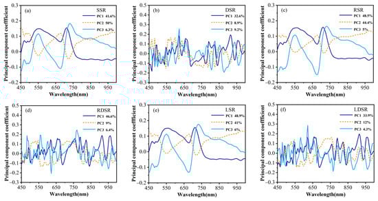
Figure 7.
The first three principal components (PCS) of PLSR explained the highest variance ratio of the different spectral regions obtained from the different data sets: (a) SSR, (b) DSR, (c) RSR, (d) RDSR, (e) LSR, (f) LDSR.
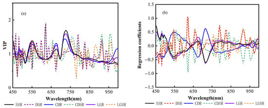
Figure 8.
The PLSR model of leaf reflectance at 450–998 nm was used to analyze the weights of the variables related to canopy SPAD evaluation in the different data sets. (a) The VIP scores across different spectral regions for each PLSR model in different data sets, (b) the regression coefficients at 450–998 nm for the summer maize SPAD value assessment using the PLSR model in different datasets.
The contribution of each band of the full-wave band remote sensing image to the RF model (Figure 9) showed how the bands related to the SPAD values supported the predictive ability of the model. When analyzing the performance of the model, this information was taken into account to verify the sensitive characteristic bands obtained by the dimension reduction algorithm. The results returned from the contribution rate of the RF model showed that, in the red edge range of the spectrum, 714 nm (5.9%), 718 nm (5.5%), and 450 nm (4.5%) of blue, 566 nm (1.6%) of green, and 998 nm (2.8%) of near-infrared were higher, and the top 20 of 138 bands accounted for more than 51% of the contribution.
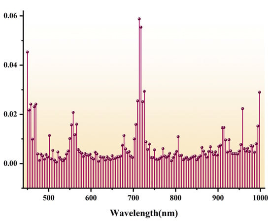
Figure 9.
RF contribution rate evaluation results of SSR data.
A series of decision trees were constructed based on the random forest model of the full-wave inversion of the summer maize SPAD values. The regression results were obtained by voting the results of each tree and did not depend on a specific single decision tree. Figure 10 shows a representative tree among the multiple decision trees, which helped to describe the relationship between common effects.
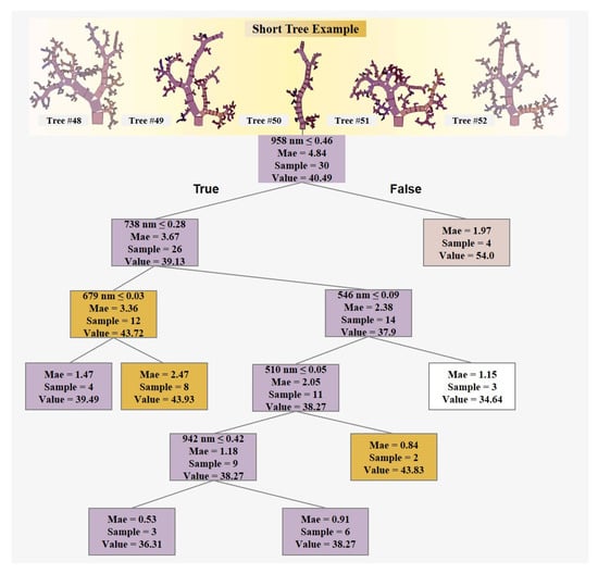
Figure 10.
Example of an RF model single decision tree (initial level 6).
Similar to the RF model, XGBoost could directly gauge the importance of each variable. “Importance” measured the value of the variables in the construction of the tree. In the summer maize SPAD values hyperspectral estimation model, the more times a band was used to build a decision tree, the more important it was. The band importance obtained by the XGBoost algorithm is shown in Figure 11. From this, it can be seen that the bands with higher importance were concentrated between 550 and 566 nm, which overlapped with the bands with a higher correlation. The importance was reduced at around 714 nm in the spectral red-light range but increased at 706 nm. The first 20 bands of the 138 bands accounted for over 67% of the contribution value. The DNN model added the full band spectral data of the training samples to the model through the input layer (Figure 12) and finally obtained the inversion model of the summer maize SPAD values.
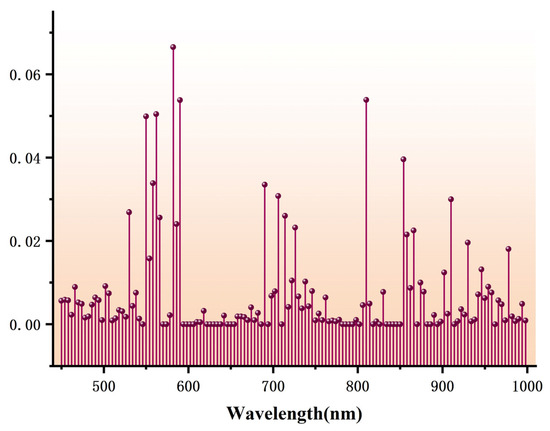
Figure 11.
XGBoost contribution rate evaluation results of the SSR data.
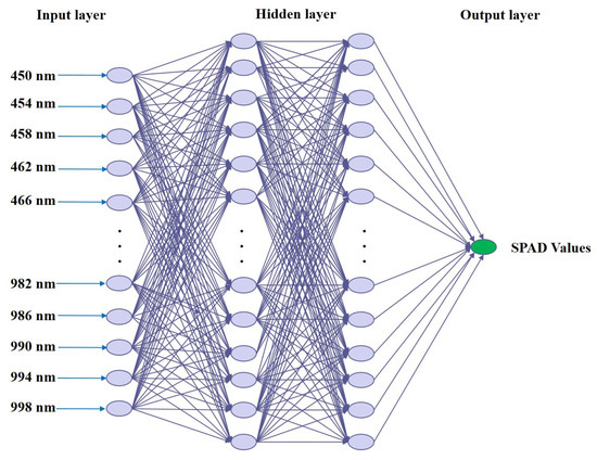
Figure 12.
DNN model structure.
Using SSR, DSR, RSR, RDSR, LSR, and LDSR, among other spectral transformation data, the characteristic bands were assigned to the parameters of the regression model. The regression algorithms, namely PLSR, RF, XGBoost, and DNN, were used to construct the maize SPAD values inversion model, the inversion accuracy of which was then verified. As shown in Figure 13, marked differences were observed in the accuracy of the inversion model based on the characteristic bands.
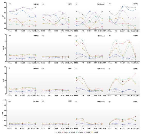
Figure 13.
Comparison of SPAD values estimation accuracy for summer maize using UAV data and four ML models: (a–d) R2, (e–h) root mean square error (RMSE), (i–l) mean absolute error (MAE), (m–p) mean relative error (MRE).
As shown in Figure 13, in the PLSR model constructed using the characteristic bands selected by FD in the DSR as the input, the R2, RMSE, MAE, and MRE were 0.36, 5, 3.91, and 0.09, respectively. In the RF model constructed based on the characteristic bands selected by full-wave in the DSR, the R2, RMSE, MAE, and MRE were 0.42, 4, 2.9, and 0.07, respectively. Further analysis was performed on the model constructed by using the XGBoost method, and the XGBoost model based on the characteristic bands selected by FD in the LDSR also showed poor performance, where the R2, RMSE, MAE, and MRE were 0.38, 9.7, 8.06, and 0.18, respectively. From the above results, based on the summer maize SPAD values inversion model constructed by differential spectral transformation (DSR, RDSR, and LDSR), the model showed poor stability and accuracy. In contrast, in the SSR, RSR, and LSR spectral transformations, the accuracy and stability of the model based on SSR were relatively high. The R2 of the SSR in the PLSR model in the CARS, SPA, and CARS_SPA characteristic band selection methods were 0.80, 0.75, and 0.81, respectively.
The verification accuracy of the LSR spectral transformation in the RF regression model was higher than that of the SSR and CSR spectral transformations. The R2 of LSR in the SPA characteristic band selection method was 0.6, with an RMSE of 2.65. In the XGBoost model, the highest SSR values in the Full, FD, and CARS_SPA characteristic band selection methods were 0.66, 0.53, and 0.65, respectively, with an RMSE of 2.5, 4.0, and 2.6, respectively. In the DNN model, the highest SSR values in the Full, SPA, and CARS_SPA characteristic band selection methods were 0.66, 0.82, and 0.82. respectively, with an RMSE of 2.78, 1.85, and 1.85, respectively, and MAE of 2.50, 3.57, and 1.56, respectively, and an MRE of 0.06, 0.08, and 0.03, respectively. These accuracy verification results indicated that the model stability of the SSR characteristic band was good. Thus, to summarize, among the three estimation models of PLSR, XGBoost, and DNN, the CARS_SPA characteristic band selection method was the most helpful in terms of improving the estimation ability of the SPAD values of the summer maize canopy.
3.4. Visual Mapping of Maize SPAD Values Based on Optimal Characteristic Bands Algorithm
According to the accuracy evaluation results (Figure 13), the accuracy of the SPAD values inversion model built based on the CART_SPA algorithm was the best among the four ML regression models. Therefore, after selecting this model, each pixel point of the 10 characteristic band images selected by the hyperspectral CARS_SPA algorithm collected on July 30 was substituted as the model input parameter into the PLSR, RF, XGBOOST, and DNN prediction models to obtain the SPAD values of each pixel point in the experimental area. From this, the grid was reclassified for display, and a visualization map of the summer maize SPAD values was obtained. To highlight the effects of the model, the full band image was also input into the four ML models as model parameters. The visualization map of the summer maize SPAD values of the full band image under SSR spectral data is shown in Figure 14. From the visualizations of the four models, it can be seen that the visualizations of the PLSR and DNN estimates with higher verification accuracies were closer to reality.
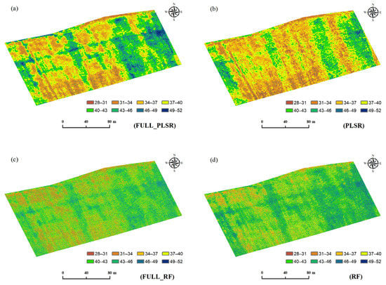
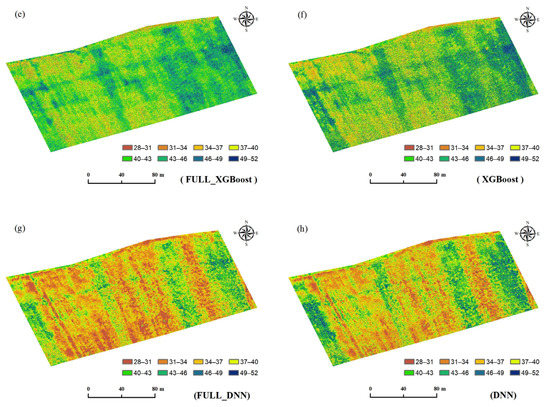
Figure 14.
Inversion diagram of SPAD values: (a) the PLSR model based on the full-wave spectral in the SSR, (b) the PLSR model based on the characteristic band selected by CARS_SPA in the SSR, (c) the RF model based on the full-wave spectral in the SSR, (d) the RF model based on the characteristic band selected by CARS_SPA in the SSR, (e) the XGBoost model based on the full-wave spectral in the SSR, (f) the XGBoost model based on the characteristic band selected by CARS_SPA in the SSR, (g) the DNN model based on the characteristic band selected by CARS_SPA in the SSR, the PLSR model based on the full-wave spectral in the SSR, (h) the DNN model based on the characteristic band selected by CARS_SPA in the SSR.
Similarly, Figure 15 presents the hyperspectral images of 12 August and 28 August input into the DNN model trained by the CARS_SPA algorithm, which were used to obtain a visualization map of the SPAD values for the two periods. According to the visualization map of the summer maize canopy SPAD values in the three growth periods, the SPAD values of the summer maize canopy in the different growth periods appeared markedly different, wherein the micro-strip drip irrigation in the three growth periods was blocked. This indicated that water conservation irrigation is the key to the growth of crops. Ensuring a continuous water supply not only promotes the growth and development of crops but also improves their yield and quality.
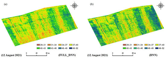
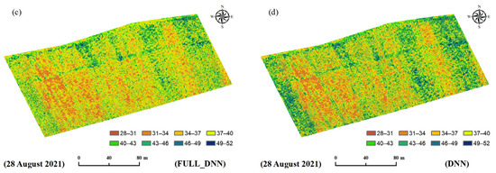
Figure 15.
SPAD value map based on optimal DNN inversion model: (a) based on full-wave inverse map of summer maize SPAD values in heading stage; (b) based on the CARS_SPA method inverse map of summer maize SPAD values in heading stage; (c) based on full-wave inverse map of summer maize SPAD values in milky maturity stage; (d) based on the CARS_SPA method of inverse map of summer maize SPAD values in milky maturity stage.
4. Discussion
Chlorophyll allows plants to absorb and transform light energy, whose content directly determines the photosynthetic capacity of plants. SPAD-502 Plus can be used to obtain SPAD values, which represent the chlorophyll content, promptly and without damaging the vegetation itself. As such, SPAD values can be used to replace traditional methods to measure chlorophyll content [39]. Our results showed that the SPAD values of the summer maize canopy in the different growth periods gradually decreased with an increase in the blockage degree of the micro-drip irrigation belts, which was consistent with previous studies on maize under drought conditions. This was because water stress affects the normal physiological function of crops by hindering the biosynthesis of chlorophyll in leaves and promoting the accelerated decomposition of existing chlorophyll, resulting in a reduction in the chlorophyll content in leaves [40]. From the jointing to tasseling stages, the chlorophyll content of the maize leaves increased with the advancing of the growth stage under different degrees of drip irrigation belt blockage. However, from the tasseling stage to the milky maturity stage, and then to the mature stage, the chlorophyll content of the maize leaves under different blockage degrees gradually decreased, as shown in Figure 14h and Figure 15 [41]. This was attributed to the fact that, in the vegetative growth stage, the maize grew vigorously, its leaves expanded, and its chlorophyll content increased. After the milky maturity stage, the summer maize entered the reproductive growth stage, the leaves began to yellow and drop, and the chlorophyll content decreased. Therefore, chlorophyll is an important indicator of plant growth, which has a good correlation with the plant development stage, of which it can be regarded as an indicator [42].
At present, research on the UAV remote sensing monitoring of food crops is scarce. However, the present study attempted to address the lack of research on food crops in northwest China and provides theoretical support for subsequent related research. In this study, Hohhot City was selected as the study site to analyze the characteristics of UAV remote sensing technology on the SPAD values of summer maize. Previous studies have shown that mathematical transformation can significantly improve the sensitivity of the vegetation spectrum to chlorophyll content [43,44], especially when high-frequency information is transformed using differential transformation. However, in this study, in Section 3.3, the precision verification results of the multiple models in Figure 13 showed that the model built by differential transformation had poor precision and stability. The verification results of mean absolute error and mean relative error showed that the accuracy of the estimation model of differential transformation was less than its data under the same estimation model. The precision verification method better highlighted the conclusion that the differential transformation estimation model had poor stability in this test area. This was mainly due to the influence of the geographical environment and climatic conditions, as the hyperspectral data of UAV contained a lot of noise. Reducing the signal-to-noise ratio of the spectral information resulted in a large amount of noise, which led to poor model stability, affecting the accuracy of the SPAD value estimation. This indicated that the extraction algorithm of high-frequency information was not suitable for the processing and analysis of the vegetation spectral information in this study test site. As such, further studies are needed to identify potential new processing methods.
In the full-wave band, the characteristic bands extracted using the CARS and SPA algorithms all had bands around 714 nm, which was consistent with the results of the random forest calculation of the contribution rate of each band and was consistent with previous studies [40,43]. In general, the narrow-band hyperspectral images selected by the CARS and SPA bands were independent of the wide-band multispectral images, and the crop spectral information obtained from the wide-band was not conducive to data depth mining. Hyperspectral images reflect more subtly the differences in the physical structure and chemical composition of crops. These characteristics determine the unique advantages of hyperspectral image technology in crop phenotype research [45]. In this context, the selection of the optimal regression model has a large impact on the estimation accuracy of SPAD values. In this study, four machine learning methods were tested to build a model with which to estimate the SPAD values of summer maize.
Compared to the PLSR, RF, and XGBoost models, the DNN model was superior in terms of spatial changes. The DNN-based model showed regional spatial adaptability in the selection methods of the SSR spectral data in various characteristic bands. It is worth noting that the PLSR model had a significantly higher accuracy in the inversion of SPAD values, indicating that the PLSR model was superior to the other models. PLSR simulates the potential linear relationship between the input variables and the modeling target. However, it was found to perform poorly on nonlinear and complex data sets and exhibited marked spatial differences in the spatial prediction of the full-wave band and the visualization map of the summer maize SPAD values retrieved using the CARS_SPA method. In contrast, XGBoost showed advantages including high efficiency, flexibility, and portability. In this study, when the number of samples was small [46], the inversion accuracy (R2) in the full-wave SSR data reached 0.66. However, compared with PLSR and DNN, the inversion accuracy was poor. Among the four models, the RF model performed the most poorly, with a higher accuracy in the remote sensing regional scale land use classification and a lower accuracy in the regression modeling. By adjusting the optimal parameters, the dependence on multiple variables was greatly reduced, and most of the defects in the existing modeling methods were resolved. The inversion model based on the CARS_SPA characteristic band selection algorithm used to extract the SSR data of 10 characteristic bands and DNN performed the best, showing a high estimation accuracy and stability. Therefore, for the hyperspectral remote sensing of UAV, the modeling and prediction of the summer maize SPAD values by DNN appeared to be the most reliable method [47].
Next, we estimated the SPAD values from the hyperspectral data of UAV and compared the four machine learning methods. In the future, other potential estimation models should be explored. In addition, there is also a need to combine multi-point analysis to obtain more samples and build a more general and applicable model. In this study, the hyperspectral data of UAV was mainly used as the data source as opposed to satellite image data, although satellite image data ensures the accurate detection of regional scale land surface information. Therefore, this study provides a basis for future studies to develop methods using satellite image data to accurately detect regional vegetation information.
5. Conclusions
In this study, the chlorophyll content of summer maize was selected as the research object, and the measured hyperspectral and SPAD value data of UAV were used as the data sources. First, the spectral transformation algorithm was selected to process and analyze the canopy spectral data. Then, the sensitive characteristic bands were extracted from the processed spectral data and the measured SPAD values data using the characteristic band selection algorithm. Finally, a model to estimate the SPAD values of summer maize was constructed using the PLSR, RF, XGBoost, and DNN algorithms. In response to the complex geographical environments and climate conditions, the summer maize canopy spectral data were found to contain a lot of noise. In this context, the high-frequency information extracted by the mathematical transformation algorithm had a weak ability to estimate the summer maize SPAD values. Compared with the high-frequency information (DSR, LDSR, and RDSR), the low-frequency information (SSR, LSR, and RSR) had a strong ability to estimate the chlorophyll content in the summer maize. Among these, the summer maize SPAD values inversion model constructed using the CARS_SPA characteristic band selection algorithm and the DNN model for SSR data showed the best performance, with a high estimation accuracy and stability (R2 = 0.82, RMSE = 1.85, MAE = 1.56, and MRE = 0.03). Thus, in this study, through a combination of the characteristic band selection algorithm and machine learning methods, the SPAD values of summer maize were effectively and quantitatively analyzed.
Author Contributions
Conceptualization, B.S. and G.R.; methodology, B.S.; software, B.S.; validation, B.S. and J.Z.; formal analysis, B.S. and G.R.; investigation, B.S. and K.L.; resources, Y.G. and S.G.; data curation, B.S.; writing—original draft preparation, B.S.; writing—review and editing, Y.B. and F.Z.; visualization, B.S.; supervision, J.Z.; project administration, J.Z.; funding acquisition, J.Z. All authors have read and agreed to the published version of the manuscript.
Funding
This study was supported by the National K&D Program of China (2019YFD1002201), the National Natural Science Foundation of China (U21A2040), the National Natural Science Foundation of China (41877520), the National Natural Science Foundation of China (42077443), the Industrial technology research and development project supported by the Development and Reform Commission of Jilin Province (2021C044-5), the Key Research and Projects Development Planning of Jilin Province (20200403065SF), and the Construction Project of Science and Technology innovation (20210502008ZP).
Conflicts of Interest
The authors declare no conflict of interest.
References
- Croft, H.; Chen, J.M.; Wang, R.; Mo, G.; Luo, S.; Luo, X.; He, L.; Gonsamo, A.; Arabian, J.; Zhang, Y.; et al. The global distribution of leaf chlorophyll content. Remote Sens. Environ. 2020, 236, 111479. [Google Scholar] [CrossRef]
- Darvishzadeh, R.; Skidmore, A.; Schlerf, M.; Atzberger, C. Inversion of a radiative transfer model for estimating vegetation LAI and chlorophyll in a heterogeneous grassland. Remote Sens. Environ. 2008, 112, 2592–2604. [Google Scholar] [CrossRef]
- Han, L.; Guijun, Y.; Dai, H.-y.; Xu, B.; Yang, H.; Feng, H.; Li, Z.; Xiaodong, Y. Modeling maize above-ground biomass based on machine learning approaches using UAV remote-sensing data. Plant Methods 2019, 15, 10. [Google Scholar] [CrossRef]
- Zheng, H.; Cheng, T.; Li, D.; Zhou, X.; Yao, X.; Tian, Y.; Cao, W.; Zhu, Y. Evaluation of RGB, Color-Infrared and Multispectral Images Acquired from Unmanned Aerial Systems for the Estimation of Nitrogen Accumulation in Rice. Remote Sens. 2018, 10, 824. [Google Scholar] [CrossRef]
- Zhou, X.; Zheng, H.B.; Xu, X.Q.; He, J.Y.; Ge, X.K.; Yao, X.; Cheng, T.; Zhu, Y.; Cao, W.X.; Tian, Y.C. Predicting grain yield in rice using multi-temporal vegetation indices from UAV-based multispectral and digital imagery. ISPRS J. Photogramm. 2017, 130, 246–255. [Google Scholar] [CrossRef]
- Arroyo-Mora, J.P.; Kalacska, M.; Løke, T.; Schläpfer, D.; Coops, N.C.; Lucanus, O.; Leblanc, G. Assessing the impact of illumination on UAV pushbroom hyperspectral imagery collected under various cloud cover conditions. Remote Sens. Environ. 2021, 258, 112396. [Google Scholar] [CrossRef]
- Belwalkar, A.; Poblete, T.; Longmire, A.; Hornero, A.; Hernandez-Clemente, R.; Zarco-Tejada, P.J. Evaluation of SIF retrievals from narrow-band and sub-nanometer airborne hyperspectral imagers flown in tandem: Modelling and validation in the context of plant phenotyping. Remote Sens. Environ. 2022, 273, 112986. [Google Scholar] [CrossRef]
- Li, Z.; Zhao, Y.; Taylor, J.; Gaulton, R.; Jin, X.; Song, X.; Li, Z.; Meng, Y.; Chen, P.; Feng, H.; et al. Comparison and transferability of thermal, temporal and phenological-based in-season predictions of above-ground biomass in wheat crops from proximal crop reflectance data. Remote Sens. Environ. 2022, 273, 112967. [Google Scholar] [CrossRef]
- Deng, L.; Mao, Z.; Li, X.; Hu, Z.; Duan, F.; Yan, Y. UAV-based multispectral remote sensing for precision agriculture: A comparison between different cameras. ISPRS J. Photogramm. 2018, 146, 124–136. [Google Scholar] [CrossRef]
- Mao, Z.-H.; Deng, L.; Duan, F.-Z.; Li, X.-J.; Qiao, D.-Y. Angle effects of vegetation indices and the influence on prediction of SPAD Values in soybean and maize. Int. J. Appl. Earth. Obs. 2020, 93, 102198. [Google Scholar] [CrossRef]
- Lu, J.; Cheng, D.; Geng, C.; Zhang, Z.; Xiang, Y.; Hu, T. Combining plant height, canopy coverage and vegetation index from UAV-based RGB images to estimate leaf nitrogen concentration of summer maize. Biosyst. Eng. 2021, 202, 42–54. [Google Scholar] [CrossRef]
- Shao, G.; Han, W.; Zhang, H.; Liu, S.; Wang, Y.; Zhang, L.; Cui, X. Mapping maize crop coefficient Kc using random forest algorithm based on leaf area index and UAV-based multispectral vegetation indices. AGR. Water. Manag. 2021, 252, 106906. [Google Scholar] [CrossRef]
- Zhang, L.; Zhang, H.; Han, W.; Niu, Y.; Chávez, J.L.; Ma, W. Effects of image spatial resolution and statistical scale on water stress estimation performance of MGDEXG: A new crop water stress indicator derived from RGB images. AGR. Water Manag. 2022, 264, 107506. [Google Scholar] [CrossRef]
- Guo, Y.; Yin, G.; Sun, H.; Wang, H.; Chen, S.; Senthilnath, J.; Wang, J.; Fu, Y. Scaling Effects on Chlorophyll Content Estimations with RGB Camera Mounted on a UAV Platform Using Machine-Learning Methods. Sensors 2020, 20, 5130. [Google Scholar] [CrossRef] [PubMed]
- Ramos, A.P.M.; Osco, L.P.; Furuya, D.E.G.; Gonçalves, W.N.; Santana, D.C.; Teodoro, L.P.R.; Junior, C.A.D.S.; Capristo-Silva, G.F.; Li, J.; Baio, F.H.R.; et al. A random forest ranking approach to predict yield in maize with uav-based vegetation spectral indices. Comput. Electron. Agr. 2020, 178, 105791. [Google Scholar] [CrossRef]
- Ishengoma, F.S.; Rai, I.A.; Said, R.N. Identification of maize leaves infected by fall armyworms using UAV-based imagery and convolutional neural networks. Comput. Electron. Agr. 2021, 184, 106124. [Google Scholar] [CrossRef]
- Lu, H.; Cao, Z.; Xiao, Y.; Fang, Z.; Zhu, Y. Toward Good Practices for Fine-Grained Maize Cultivar Identification With Filter-Specific Convolutional Activations. IEEE T Autom. Sci. Eng. 2018, 15, 430–442. [Google Scholar] [CrossRef]
- Guo, Y.; Chen, S.; Li, X.; Cunha, M.; Jayavelu, S.; Cammarano, D.; Fu, Y. Machine Learning-Based Approaches for Predicting SPAD Values of Maize Using Multi-Spectral Images. Remote Sens. Environ. 2022, 14, 1337. [Google Scholar] [CrossRef]
- Galvão, R.K.H.; Araújo, M.C.U.; Fragoso, W.D.; Silva, E.C.; José, G.E.; Soares, S.F.C.; Paiva, H.M. A variable elimination method to improve the parsimony of MLR models using the successive projections algorithm. Chemometr. Intell. Lab. 2008, 92, 83–91. [Google Scholar] [CrossRef]
- Aladejana, O.O.; Salami, A.T.; Adetoro, O.-I.O. Hydrological responses to land degradation in the Northwest Benin Owena River Basin, Nigeria. J. Environ. Manag. 2018, 225, 300–312. [Google Scholar] [CrossRef]
- Wold, S.; Esbensen, K.; Geladi, P. Principal component analysis. Chemometr. Intell. Lab. 1987, 2, 37–52. [Google Scholar] [CrossRef]
- Chen, Z.; Jia, K.; Xiao, C.; Wei, D.; Zhao, X.; Lan, J.; Wei, X.; Yao, Y.; Wang, B.; Sun, Y.; et al. Leaf Area Index Estimation Algorithm for GF-5 Hyperspectral Data Based on Different Feature Selection and Machine Learning Methods. Remote Sens. 2020, 12, 2110. [Google Scholar] [CrossRef]
- Jia, M.; Li, W.; Wang, K.; Zhou, C.; Cheng, T.; Tian, Y.; Zhu, Y.; Cao, W.; Yao, X. A newly developed method to extract the optimal hyperspectral feature for monitoring leaf biomass in wheat. Comput. Electron. Agr. 2019, 165, 104942. [Google Scholar] [CrossRef]
- Khaled, A.Y.; Abd Aziz, S.; Khairunniza Bejo, S.; Mat Nawi, N.; Jamaludin, D.; Ibrahim, N.U.A. A comparative study on dimensionality reduction of dielectric spectral data for the classification of basal stem rot (BSR) disease in oil palm. Comput. Electron. Agr. 2020, 170, 105288. [Google Scholar] [CrossRef]
- Samsudin, S.H.; Shafri, H.; Hamedianfar, A. Development of spectral indices for roofing material condition status detection using field spectroscopy and WorldView-3 data. J. Appl. Remote Sens. 2016, 10, 25021. [Google Scholar] [CrossRef]
- Zhang, S.; Shen, Q.; Nie, C.; Huang, Y.; Wang, J.; Hu, Q.; Ding, X.; Zhou, Y.; Chen, Y. Hyperspectral inversion of heavy metal content in reclaimed soil from a mining wasteland based on different spectral transformation and modeling methods. Spectrochim. Acta A 2019, 211, 393–400. [Google Scholar] [CrossRef]
- Malone, B.M.; Tan, F.; Bridges, S.M.; Peng, Z. Comparison of four ChIP-Seq analytical algorithms using rice endosperm H3K27 trimethylation profiling data. PLoS ONE 2011, 6, e25260. [Google Scholar] [CrossRef]
- Li, H.; Liang, Y.; Xu, Q.; Cao, D. Key wavelengths screening using competitive adaptive reweighted sampling method for multivariate calibration. Anal. Chim. Acta 2009, 648, 77–84. [Google Scholar] [CrossRef]
- Su, W.-H.; Bakalis, S.; Sun, D.-W. Fourier transform mid-infrared-attenuated total reflectance (FTMIR-ATR) microspectroscopy for determining textural property of microwave baked tuber. J. Food Eng. 2018, 218, 1–13. [Google Scholar] [CrossRef]
- Rischbeck, P.; Elsayed, S.; Mistele, B.; Barmeier, G.; Heil, K.; Schmidhalter, U. Data fusion of spectral, thermal and canopy height parameters for improved yield prediction of drought stressed spring barley. Eur. J. Agron. 2016, 78, 44–59. [Google Scholar] [CrossRef]
- Aghighi, H.; Azadbakht, M.; Ashourloo, D.; Shahrabi, H.; Radiom, S. Machine Learning Regression Techniques for the Silage Maize Yield Prediction Using Time-Series Images of Landsat 8 OLI. IEEE J. Sel. Top. Appl. Earth Obs. Remote Sens. 2018, 11, 4563–4577. [Google Scholar] [CrossRef]
- Ndlovu, H.S.; Odindi, J.; Sibanda, M.; Mutanga, O.; Clulow, A.; Chimonyo, V.G.P.; Mabhaudhi, T. A Comparative Estimation of Maize Leaf Water Content Using Machine Learning Techniques and Unmanned Aerial Vehicle (UAV)-Based Proximal and Remotely Sensed Data. Remote Sens. 2021, 13, 4091. [Google Scholar] [CrossRef]
- Wang, J.; Zhou, Q.; Shang, J.; Liu, C.; Zhuang, T.; Ding, J.; Xian, Y.; Zhao, L.; Wang, W.; Zhou, G.; et al. UAV- and Machine Learning-Based Retrieval of Wheat SPAD Values at the Overwintering Stage for Variety Screening. Remote Sens. 2021, 13, 5166. [Google Scholar] [CrossRef]
- Chen, B.; Mu, X.; Chen, P.; Wang, B.; Choi, J.; Park, H.; Xu, S.; Wu, Y.; Yang, H. Machine learning-based inversion of water quality parameters in typical reach of the urban river by UAV multispectral data. Ecol. Indic. 2021, 133, 108434. [Google Scholar] [CrossRef]
- Moghimi, A.; Pourreza, A.; Zuniga-Ramirez, G.; Williams, L.E.; Fidelibus, M.W. A Novel Machine Learning Approach to Estimate Grapevine Leaf Nitrogen Concentration Using Aerial Multispectral Imagery. Remote Sens. 2020, 12, 3515. [Google Scholar] [CrossRef]
- Wei, L.; Wang, Z.; Huang, C.; Zhang, Y.; Wang, Z.; Xia, H.; Cao, L. Transparency Estimation of Narrow Rivers by UAV-Borne Hyperspectral Remote Sensing Imagery. IEEE Access 2020, 8, 168137–168153. [Google Scholar] [CrossRef]
- Zhang, Y.; Xia, C.; Zhang, X.; Cheng, X.; Feng, G.; Wang, Y.; Gao, Q. Estimating the maize biomass by crop height and narrowband vegetation indices derived from UAV-based hyperspectral images. Ecol. Indic. 2021, 129, 107985. [Google Scholar] [CrossRef]
- Lai, Y.-C.; Huang, Z.-Y. Detection of a Moving UAV Based on Deep Learning-Based Distance Estimation. Remote Sens. 2020, 12, 3035. [Google Scholar] [CrossRef]
- Hawkins, T.S.; Gardiner, E.S.; Comer, G.S. Modeling the relationship between extractable chlorophyll and SPAD-502 readings for endangered plant species research. J. Nat. Conserv. 2009, 17, 123–127. [Google Scholar] [CrossRef]
- Zhu, W.; Sun, Z.; Yang, T.; Li, J.; Peng, J.; Zhu, K.; Li, S.; Gong, H.; Lyu, Y.; Li, B.; et al. Estimating leaf chlorophyll content of crops via optimal unmanned aerial vehicle hyperspectral data at multi-scales. Comput. Electron. Agr. 2020, 178, 105786. [Google Scholar] [CrossRef]
- Mulero, G.; Bacher, H.; Kleiner, U.; Peleg, Z.; Herrmann, I. Spectral Estimation of In Vivo Wheat Chlorophyll a/b Ratio under Contrasting Water Availabilities. Remote Sens. 2022, 14, 2585. [Google Scholar] [CrossRef]
- Peng, Y.; Nguy-Robertson, A.; Arkebauer, T.; Gitelson, A.A. Assessment of Canopy Chlorophyll Content Retrieval in Maize and Soybean: Implications of Hysteresis on the Development of Generic Algorithms. Remote Sens. 2017, 9, 226. [Google Scholar] [CrossRef]
- Li, D.; Cheng, T.; Zhou, K.; Zheng, H.; Yao, X.; Tian, Y.; Zhu, Y.; Cao, W. WREP: A wavelet-based technique for extracting the red edge position from reflectance spectra for estimating leaf and canopy chlorophyll contents of cereal crops. ISPRS J. Photogramm. 2017, 129, 103–117. [Google Scholar] [CrossRef]
- Liao, Q.; Wang, J.; Guijun, Y.; Zhang, D.; Li, H.; Fu, Y.; Li, Z. Comparison of spectral indices and wavelet transform for estimating chlorophyll content of maize from hyperspectral reflectance. J. Appl. Remote Sens. 2013, 7, 3575. [Google Scholar] [CrossRef]
- Zhang, Y.; Hui, J.; Qin, Q.; Sun, Y.; Zhang, T.; Sun, H.; Li, M. Transfer-learning-based approach for leaf chlorophyll content estimation of winter wheat from hyperspectral data. Remote Sens. Environ. 2021, 267, 112724. [Google Scholar] [CrossRef]
- Shu, M.; Shen, M.; Zuo, J.; Yin, P.; Wang, M.; Xie, Z.; Tang, J.; Wang, R.; Li, B.; Yang, X.; et al. The Application of UAV-Based Hyperspectral Imaging to Estimate Crop Traits in Maize Inbred Lines. Plant Phenomics 2021, 2021, 9890745. [Google Scholar] [CrossRef]
- Maimaitijiang, M.; Sagan, V.; Sidike, P.; Hartling, S.; Esposito, F.; Fritschi, F.B. Soybean yield prediction from UAV using multimodal data fusion and deep learning. Remote Sens. Environ. 2020, 237, 111599. [Google Scholar] [CrossRef]


Publisher’s Note: MDPI stays neutral with regard to jurisdictional claims in published maps and institutional affiliations. |
© 2022 by the authors. Licensee MDPI, Basel, Switzerland. This article is an open access article distributed under the terms and conditions of the Creative Commons Attribution (CC BY) license (https://creativecommons.org/licenses/by/4.0/).