Article

Climatology of TEC Longitudinal Difference in Middle Latitudes of East Asia

1
China Research Institute of Radiowave Propagation (CRIRP), Qingdao 266107, China
2
Department of Space Physics, School of Electronic Information, Wuhan University, Wuhan 430072, China
3
School of Physics, Xidian University, Xi’an 710126, China
4
Beijing Institute of Applied Meteorology, Beijing 100029, China
*
Author to whom correspondence should be addressed.
Remote Sens. 2022, 14(21), 5412; https://doi.org/10.3390/rs14215412
Submission received: 29 September 2022 / Revised: 24 October 2022 / Accepted: 26 October 2022 / Published: 28 October 2022
(This article belongs to the Section Atmospheric Remote Sensing)

Abstract

:
In this paper, a statistical analysis of the diurnal, seasonal and solar cycle variation in the TEC longitudinal difference in midlatitudes of East Asia is presented using CODE GIMs data in 2015–2019. Moreover, the empirical neutral wind model HWM-14 and geomagnetic field model IGRF-2020 were employed to analyze the influence of geomagnetic configuration-neutral wind mechanism on the TEC longitudinal difference, and the F2 layer peak electron density (NmF2) data from the Constellation Observing System for Meteorology, Ionosphere and Climate (COSMIC) were also used to study the role of local electron density in the TEC longitudinal difference. For the high solar activity year, the results show that east-west TEC longitudinal difference index Re/w is negative in the noon and positive at evening-night. Moreover, the longitudinal difference of daytime TEC is most evident in summer, less in autumn and least in spring and winter, while the nighttime difference is most obvious in equinox, followed by summer and winter during nighttime. The model simulation shows that the TEC longitude difference around noon is mainly caused by the zonal wind-declination mechanism, and a 4-h time delay seems to be an optimal result for the vertical drift velocity to cause the longitudinal TEC difference during pre-noon hours. At night, the uplifting electron flux, which is a product of local electron density and vertical drift velocity, shows a good correlation with Re/w, indicating that the local electron density is also an important factor affecting the TEC longitudinal difference during the nighttime. Moreover, there was about a 3-h time delay between the TEC longitudinal variations and the uplifting electron flux at night. For the low solar activity years, the western TEC is greater than eastern TEC during most of the year except in the summer nighttime. The TEC diurnal variation in the east and west suggested that the nighttime Re/w should be related to other physical process, such as the midlatitude summer nighttime anomaly (MSNA) in the east and the ionospheric nighttime enhancement (INE). The current study provides evidence for the longitudinal difference of NmF2 in East Asian midlatitudes and geomagnetic configuration-neutral wind mechanism proposed in previous studies and finds some new features which need further studying to improve our current understanding of ionospheric longitudinal difference in the low solar activity years. The results provide new insight into TEC longitudinal variations at midlatitudes, and they can contribute to understanding the ionosphere-thermosphere coupling system.

1. Introduction

The ionosphere is a system with complex temporal-spatial variations. The time scale of this highly coupled system varies from a few minutes to a solar cycle (~11 years). In terms of latitudinal variation, the obvious structures include equatorial ionosphere anomaly (EIA), midlatitude trough (MIT) and so on [1,2,3,4,5,6,7,8,9,10]. On the other hand, the ionospheric longitude variations show different characteristics at different latitudes. There are wave-4 structures in the equator and low latitudes [11,12,13,14], and this structure is related to the electric fields generated by nonmigrating atmospheric tides in the E-region height that vary with longitude [15,16,17,18]. In addition, longitudinal variations of midlatitude ionosphere have been studied for decades. The annual and semi-annual variations of the ionosphere at different longitudes can be explained by the differences between the geomagnetic poles and the solar zenith angle variations [19,20]. Moreover, the nighttime enhancement in NmF2 was believed to be caused by the neutral winds combined with geomagnetic field configuration based on the low-orbit satellite in situ Ne data [21,22]. A new class of midlatitudes ionospheric longitudinal difference has been researched in recent decades [23,24,25,26,27,28,29,30,31,32,33,34]. The neutral wind would push the plasma up or down along the magnetic field due to non-zero magnetic declination. As the recombination rates are higher in the low altitudes, electron densities are decreased. Due to the longitudinal variation of the magnetic declination angle, the zonal wind would drive the plasma with different vertical velocities at different longitudes. Therefore, TEC and electron densities would exhibit longitudinal differences.
In the study of longitudinal variation of ionosphere, previous studies have carried out investigations using electron density and hmF2 [26,35]. Zhang et al. [23] first discovered the TEC longitudinal difference in the North American middle latitudes based on the GPS TEC data in the US mainland. That is, during the morning and early afternoon, the midlatitudes TEC in the western longitude was larger than that in the eastern longitude. They also suggested the zonal wind-magnetic declination mechanism to explain the phenomenon. Then, Xu et al. [28] verified that the TEC longitudinal differences also exist at North America, South America and Oceania midlatitudes. Moreover, Zhao et al. [27] used the NmF2 and COSMIC RO data in the Far Eastern area to identify longitudinal variations in midlatitudes F-region electron density. Furthermore, Zhang et al. [24] reported that there is a strong correlation between the Fabry-Perot interferometer (FPI) wind data and the West-East (92°W–51°W GLon) differences in electron density supporting the zonal wind-geomagnetic declination mechanism. Besides, Zhang et al. [26] reported a good correlation between spatial variations in the second EOF mode and the vertical plasma drift caused by the zonal wind over America in their analysis of a 12-year ground-based American longitude sector GPS TEC dataset. They further strongly suggest a causative mechanism involving varying declination with longitude along with varying zonal wind climatology with local time, season and solar cycle. Yao et al. [36] also found a similar correlation based on the TEC dataset over North America and East Asia. Ren et al. [33] suggested that the zonal wind significantly influences the ionospheric east-west differences in the mid-latitude of the Far Eastern region using the TIME3D-IGGCAS model. In addition to the magnetic declination-zonal wind effects described above, Luan and Dou [34] suggested that the magnetic inclination-meridional wind mechanism should also be responsible for the midlatitude variation in the southern hemisphere during the night time. Wang et al. [30] also demonstrated that the meridional wind, migrating tides from the lower ionosphere and solar illumination could also affect the longitudinal structure of F-region Ne at mid-latitudes based on the simulation results of global ionosphere-thermosphere model (GITM) simulation and CHAMP observations. Moreover, there are a number of studies on the climatology of plasmaspheric TEC for the coupling processes between the ionosphere and the plasmasphere is known to greatly influence not only the plasmaspheric density but also the ionospheric density [37,38].
The study of TEC characteristics is crucial to the ionosphere-thermosphere system, since TEC is the primary factor contributing to the extra time delay in satellite signal propagation [39,40]. In previous studies, Zhang et al. [23] analyzed the US continent TEC differences and Xu et al. [28] analyzed South America, North America and Oceania. Until now, no specific studies have analyzed the climatology of TEC longitudinal difference in East Asia. Therefore, to investigate the characteristics of TEC longitudinal differences in the East Asian midlatitude, this paper employed TEC data from the International GNSS Service (IGS) database from 2015 to 2019. This work can help to the understanding of ionosphere-thermosphere coupling, and it can be used to enhance the current reporting and forecasting capabilities of the ionospheric model. This paper describes the data, model and analysis methods used in Section 2. Section 3 presents the dependence of TEC longitudinal difference on solar activity, season and local time. Section 4 discusses the results. Section 5 provides a summary.

2. Data and Methods of Analysis

Global Ionospheric Maps (GIMs) obtained from the Center for Orbit Determination in Europe (CODE, [41]) (ftp:/ftp.unibe.ch/aiub/CODE/, accessed on 27 October 2020) were used in this study. The GIMs are an official product of the IGS obtained from dual-frequency observations performed at GNSS stations ([42]). The TEC in the GIMs were modeled using a spherical harmonic expansion up to degree order 15 and a solar-geomagnetic reference frame at CODE [43]. Although this technique may exclude some small-scale patterns of the TEC features, our goal here is to estimate the large-scale TEC longitudinal difference in the midlatitude of East Asia. As a consequence, the eliminations have little effect on the features of the results. Furthermore, GIM-TEC was confirmed using TOPEX/Jason TEC data in numerous studies, indicating that, while some inconsistencies exist, CODE TEC performs well in representing TOPEX/Jason TEC [44]. The CODE GIM map covers a longitude range of −180° to 180° and a latitude range of −87.5° to 87.5°, with longitudinal and latitudinal resolutions of 5° and 2.5°, respectively. The time resolution is 2 h before 2015 and 1 h after 2015. Therefore, we use the CODE GIMs data from 2015 to 2020. Because the focus of this paper is mainly on the midlatitudes of East Asia, considering the low magnetic latitude of East Asia, the equatorial anomaly may affect the low-mid latitudes [36], and the middle latitudes in the east of East Asia may be affected by the midlatitude trough at night [10]. Therefore, the Ionospheric TEC mean of 45°N–50°N was used to characterize the midlatitude ionospheric TEC in East Asia in this paper.
The COSMIC IRO data were obtained from the COSMIC Data Analysis of Archive Center (CDAAC, http://cdaac-www.cosmic.ucar.edu/cdaac/products.html, accessed on 28 September 2022), and previous studies have reported that the COSMIC NmF2 revealed good agreement with the ionosonde data and incoherent scatter radar data [45,46,47]. Since geomagnetic activity have an important effect on the ionosphere, we select the date satisfying Ap < 22 to analyze the ionospheric longitude difference in the middle latitude of East Asia and the Ap index is obtained from World Data Center (WDC, http://wdc.kugi.kyoto-u.ac.jp/, accessed on 28 September 2022). Figure 1 shows the F10.7 variations obtained from NOAA (National Oceanic and Atmospheric Administration, ftp://ftp.swpc.noaa.gov/pub/indices/old_indices/, accessed on 28 September 2022) during 2015–2020. The figure demonstrates that 2015 is a high solar activity year, whereas 2018 and 2019 are low solar activity years, and F10.7 of the whole year does not exceed 100. Therefore, when studying the influence of solar activity on the ionospheric longitude effect, we used TEC data in 2015 and TEC data in 2018 and 2019, respectively.
Figure 2 depicts the variation of TEC in East Asia middle latitude on 10 June 2015 (geomagnetic quiet day). On this day, the maximum geomagnetic ap index is 7, the daily Ap index is 4 and the solar activity index F10.7 is 136.6. Since the time resolution of GIMs MAP is 1 h when converting local time in longitudes such as 65°E, the nearest integer local time (the local time in 60°E) is adopted. It can be seen from the figure that the TEC in different longitude show different diurnal variation. Specifically, the TEC reaches its maximum around noontime in eastern midlatitudes (60°E–110°E), while the maximum of TEC appeared after sunset in western midlatitudes (110°E–140°E). On the other hand, the TEC display different longitudinal variation at different local times. The TEC value decreases as the longitude shifts east during noontime, and it increases as the longitude shifts to east during nighttime. Therefore, western TEC is significantly larger than the eastern TEC at noon and a reverse situation applies for nighttime, consistent with previous studies. Moreover, the longitudinal difference is most prominent in the easternmost and westernmost of East Asia most of the time. According to the calculation of the IGRF2020 model, the longitude of 0° magnetic declination in the ionospheric height range (60–1000 km) of the East Asian sector is around 97°. At the same time, considering the local time conversion, we select the 45°N–50°N Ionospheric TEC to mean of 60°E and 135°E, which are almost symmetrical with 97°E to represent the TEC values in the west and east of the East Asian sector. Table 1 shows the longitude and latitude and magnetic declination/inclination of GIMs map grid points used in this paper. Consistent with the parameters used in the previous study, this paper uses the hourly east-to-west differential index Re/w to represent ionospheric longitude difference. The Re/w is calculated through the following formula:
R e / w = TEC e TEC w / 0 . 5 ( TEC e + TEC w )
where TECe and TECw are hourly TEC values in midlatitudes of 135°E and 60°E, respectively. Since geomagnetic activities are not quiet on some days as described above, the Re/w pattern during the geomagnetic quiet days which satisfying AP < 22 are divided into 288 grids according to the month division from January to December and the local time division from 0 to 23LT.
Horizontal wind model HWM-14 was utilized in this work as the wind field model, and it is mainly based on wind observations obtained from the DE 2 and AE-E satellites [48,49,50]. The model describes the wind fields according to the spatial information (longitude, latitude, altitude) and temporal information (day of year, time of day) as well as geomagnetic daily Ap index, the wind field simulated by HWM-14 thus does not change with solar activity. Besides, the model has been updated with new observations and formulation changes. These new observations include FPI measurements and the Gravity Field and Steady State Ocean Circulation Explorer (GOCE) satellite observations [51]. The update HWM-14 provides an improved specification of thermospheric general circulation. Therefore, we use the HWM-14 model to calculate the atmospheric wind field on the ionospheric height.

3. Results

Figure 3 presents the diurnal variation of TEC longitude difference index Re/w in East Asia during the high solar activity year 2015. As can be seen from the figure, the western TEC is greater than the eastern one in the daytime, and this longitude difference is most significant during the noon period. From the perspective of seasonal variations, the longitudinal difference of daytime TEC is most evident in summer, less in autumn and least in spring and winter. At night, the longitude difference of Eastern TEC greater than Western TEC is most significant around midnight, and this difference is most obvious in equinox, followed by summer and winter during the pre-midnight period. On the other hand, this longitudinal difference after midnight is most significant in spring, and it is weak only in September in autumn months, indicating a semi-annual asymmetry during this period. It is worth noting that the western TEC will be even greater than the eastern TEC after midnight in late autumn and winter, and this phenomenon seems most obvious in winter.
Figure 4 presents the diurnal variation of Re/w in the East Asian midlatitude in the low solar activity years (2018/2019), and the Re/w index given in the figure is the average of the Re/w index in geomagnetic quiet days in 2018 and 2019. It shows that the western TEC is greater than eastern TEC almost all year around. Specifically, the longitude difference of the western daytime TEC greater than the eastern daytime TEC is obvious near noon, and the seasonal features is most evident in summer and autumn. In the morning around sunrise, the longitudinal difference of the western daytime TEC greater than the eastern daytime TEC is also evident in winter. In addition, the longitudinal difference of the eastern TEC greater than western TEC at night is only shown in the period before midnight in summer, and it still shows the longitude difference that the western TEC is greater than the eastern TEC in the rest of the time. The longitude difference of the western TEC greater than eastern TEC at night is most obvious in winter.
To better compare the longitude difference in different seasons of high and low solar activity years, Figure 5 takes March, June, September and December as representatives to display the patterns of Re/w in different seasons in high and low solar activity years. In general, except for 14LT in spring and 11–13LT in summer, the Re/w index in high solar activity years is higher than that in low solar activity years in any other period. Considering that the positive and negative values of Re/w represent reverse longitudinal difference, the solar activity seems not to affect both positive and negative Re/w simultaneously, which is consistent with previous studies [25,27]. Specifically, the results show that the western TEC is greater than the eastern TEC during the daytime period 09:00LT–17:00LT, while the eastern TEC is greater than the western TEC in other periods in spring. In the spring of low solar activity years, the eastern TEC is smaller than the western TEC. In summer, the Re/w displays similar variation in high and low years of solar activity. During the daytime, 06:00LT–18:00LT, the western TEC is greater than the eastern TEC, and the opposite situation is true for the nighttime. However, in the low solar activity years, the western TEC is greater than that of the eastern within 0–3LT after midnight. In autumn, the western TEC is larger than the eastern TEC except for the period before midnight in high solar activity years. In winter, the eastern TEC is greater than the western TEC in the morning and dusk periods in the high solar activity year. In other periods, the western TEC is slightly greater than the eastern TEC. Moreover, the western TEC is much larger than the eastern TEC in all periods in the low solar activity year.

4. Discussion

4.1. Comparsion with Previous Results

In the study of the longitude effect of ionospheric electron density in North America [25], it is found that the positive difference in the late evening is most obvious in winter and the negative difference in pre-noon hours is most apparent in early spring and late summer. Zhao et al. [27] reported that the longitudinal difference (Re/w) of the peak electron density (NmF2) over the Far East area is basically similar to that in the US continent (negative Re/w in the noon and positive Re/w during the nighttime). However, the comparison shows the different seasonal magnitude of Re/w: The noontime negative Re/w is most apparent from April to June in the East Asian midlatitude, whereas the nighttime positive Re/w is much less evident than in the US. These new features need further studying; some of them can also be validated by the results in this paper.
In this paper, the results show that the diurnal variation of Re/w in high solar activity is also similar to previous studies (negative Re/w at noon and positive Re/w at nighttime). Moreover, the negative Re/w during the noontime in the East Asian midlatitude seems most evident in summer, less in autumn, and least in spring and winter, consistent with the longitudinal difference of NmF2 in East Asia [27]. In the high solar activity years, the positive Re/w seems most evident equinox, followed by summer and winter. In the low solar activity years, except for a positive Re/w from sunset to midnight in summer, negative Re/w prevailed in almost all months, and it is most obvious in winter. Zhao et al. [27] also reported that the longitudinal difference of eastern NmF2 larger than western NmF2 is least evident in December, contrasting with the most evident positive Re/w in winter in the US. Therefore, the longitudinal difference of TEC in East Asia is basically consistent with the longitudinal difference of NmF2, providing evidence for the significant difference between the longitudinal difference of ionosphere in East Asia and the USA. On the other hand, the western ionosphere is greater than that of the eastern one almost all year round in low solar activity years, indicating that there are different physical mechanisms driving the ionospheric longitude difference in high and low solar activity years, especially in winter. Although Xu et al. [28] did not study the longitude difference of TEC in East Asia, they also found a similar situation in other regions in some individual years that TEC on one side of 0° magnetic declination is almost larger than TEC on the other side throughout the year, confirming that the longitude difference in the low solar activity years is not an individual phenomenon in East Asia.

4.2. Wind Field Simulation by HWM-14

In previous studies on ionospheric longitudinal differences, the neutral wind was considered to be one of the primary causes of ionospheric longitudinal differences. The main physical mechanisms can be summarized as follows. Plasma is either pulled up or down by the neutral wind projection on the magnetic field line. Additionally, the magnetic declination angle and magnetic inclination angle had an impact on the vertical drift (Vz) of the plasma generated by neutral winds. The relationship may be described as follows:
V z = sin I cos I u sin D + v cos D
where u is the geographic zonal winds, v is the geographic meridional winds, D is the magnetic declination angle and I is the magnetic inclination angle. Due to magnetic declination being positive or negative on both sides of zeros magnetic declination longitude, neutral winds would drive the plasma up/down to higher/lower altitudes along the magnetic field. Since the recombination rates are lower/higher at higher/lower altitudes, electron densities get enhanced/decreased. As a result, the electron densities and TEC exhibit longitudinal differences on the different sides of zero magnetic declination longitude.
This paper used neutral winds derived from the HWM-14 model and geomagnetic declination and inclination derived from IGRF-2020 (http://wdc.kugi.kyoto-u.ac.jp/, accessed on 28 September 2022) to evaluate the role of neutral wind and geomagnetic field in the ionospheric longitude difference in East Asia and discussed other factors which might cause ionospheric longitude difference.
Figure 6 presents the variation of vertical drift velocity at the height of 300 km at 60°E, 47.5°N and 135°E, 47.5°N calculated by Equation (2) and the corresponding vertical velocity difference. It is necessary to mention that the vertical drift velocity calculated by the HWM-14 model and IGRF 2020 model are almost identical within the height of ionospheric F2 peak height (hmF2) (250–350 km) in 60°E, 47.5°N and 135°E, 47.5°N, as shown in Figure A1. In addition, Figure 6 demonstrates that the neutral wind has a similar lifting or lowering effect on the ionospheric plasma is similar on both sides of the middle latitude in East Asia, that is, the neutral wind pushes the plasma downward during most of the daytime, while the neutral wind lifts the plasma upward during most of the night. However, the vertical velocity of plasma driven by neutral wind in the east and west are different for different seasons. For example, the plasma vertical drift driven by the neutral wind in the western midlatitude is stronger than that in the eastern midlatitude, and this phenomenon is most obvious in summer. At night, the neutral wind lifts the plasma faster in the east than in the west, and this phenomenon is most obvious in winter and least obvious in summer.

4.3. Possible Explanation for the Re/w in High Solar Activity Year

By comparing the TEC longitude difference index Re/w and the longitudinal difference of the vertical drift velocity in high solar activity years, we found that the seasonal characteristic that the western TEC greater than the eastern one around noontime seems consistent with the seasonal characteristic of the plasma velocity difference caused by neutral wind during pre-noon hours, indicating that the longitude difference at noon is significantly influenced by the neutral wind. As can be seen in Figure 3 and Figure 6, there is a time delay between the wind change and the TEC response, because neutral densities, temperatures and plasma temperatures are related to the local time, season, solar activity, height as well as other factors. These factors determine the velocity of chemical recombination, diffusion and the speed of the ions’ drift. The influence of the horizontal wind on the Ne (and TEC) differential builds up when it continues in the same direction, and its effect can be canceled when it changes the direction. Consequently, the observed TEC difference represents a cumulative result over time [24]. Considering the longitudinal difference in the daytime is most obvious at noon and the change of wind direction at sunrise period, we calculated the correlation coefficients between the vertical drift velocity difference at 6LT–8LT, 7LT–9LT, 8LT–10LT and the longitudinal index in 11LT–13LT, respectively.
As shown in Figure 7, the correlation coefficients are 0.76, 0.80 and 0.72, respectively. Moreover, the longitudinal difference of vertical drift velocity caused by neutral wind during the day seems to have a 4-h time delay for the longitudinal TEC difference in the noontime for East Asia, consistent with the previous result [32]. Therefore, a 4-h time delay seems to be an optimal result for the vertical drift velocity to cause the longitudinal TEC difference during pre-noon hours in the East Asian midlatitude in the year with high solar activity.
To further explore the contribution of meridional wind and zonal wind to the ionospheric longitude difference caused by the neutral wind velocity difference in East Asian daytime, using Equation (2), we calculated the ratio of the vertical drift velocity difference caused by meridional wind Δ ( sin I cos I U sin D ) to the total drift velocity difference Δ V z and the ratio of the vertical drift velocity difference Δ ( sin I cos I V cos D ) caused by zonal wind to the total drift velocity difference Δ V z in 7LT–9LT. As shown in Figure 8, the ratio of zonal wind vertical velocity difference to total drift velocity difference is greater than 1 in most cases, while the ratio of meridional wind vertical velocity to total drift velocity difference is less than 0 in most cases. During some periods, the zonal wind contribution is less than 1, but the ratio is still more than 0.8. These results indicate that the zonal wind-geomagnetic declination mechanism is the dominating cause for the daytime TEC longitudinal difference in the East Asian midlatitude, and meridional wind makes a small contribution and can even reduce the vertical velocity difference. In addition, we calculated the correlation coefficient between the vertical drift velocity difference caused by 7LT–9LT zonal wind and the TEC longitude index Re/w during 11LT–13LT. It is found that the correlation coefficient is 0.846, which is higher than that between the overall neutral wind velocity difference and the ionospheric longitude index Re/w, confirming that the ionospheric longitude difference around noon is mainly caused by the zonal wind-geomagnetic declination mechanism in the East Asian midlatitude.
Figure 3 also shows that the TEC longitude difference in East Asia (eastern TEC is greater than western TEC) is the most obvious around midnight, and this feature is most pronounced in equinox, followed by summer and winter in high solar activity years. Zhao et al. [27] also found similar features for the Re/w of NmF2. However, the difference of plasma vertical drift velocity caused by neutral wind in the region is the strongest in winter, followed by equinox and summer in the East Asian midlatitude. Therefore, the seasonal distribution of the TEC longitudinal difference is completely different from the difference in plasma vertical drift velocity at night. The difference between them might be related to the seasonal characteristics of ionospheric electron density Ne, as mentioned by previous studies [27,29]. Zhao et al. [27] proposed that the climatology changes in east-west asymmetry should be associated with the seasonal variations of the F region at midlatitude, and Wang et al. [29] also suggested the background electron density is crucial to the midlatitude longitudinal difference of Δ N e . Because the amount of plasma lifted by the neutral wind depends on the lifting speed and electron density at the same time, it can be described as follows:
N e l i f t = V z N e
where N e l i f t is the electron flux lifted by the neutral wind per second, V z is the vertical drift velocity and N e is the local electron density.
In order to test this hypothesis, we calculated the mean NmF2 in summer, winter and equinox in the eastern midlatitude (125°E–145°E, 45°N–50°N) and western midlatitude (50°E–70°E, 45°N–50°N) of East Asia from 2012 to 2015 based on COSMIC RO data on these two regions. It is worth noting that the vertical drift velocity is almost identical within the height of ionospheric F2 peak height (hmF2) in 60°E, 47.5°N and 135°E, 47.5°N, as shown in Figure A1, and the ionospheric electrons are mainly concentrated near the height of hmF2. Therefore, it is appropriate to use NmF2 to calculate the electron flux lifted by the neutral wind when studying the TEC longitude difference. Then, we multiply the NmF2 of 17LT–23LT, 18LT–24LT and 19LT–01LT in summer, winter and equinox by the plasma vertical drift velocity in the same season in these two regions to obtain the electron flux raised by neutral wind, and compare the difference between them with longitudinal difference index Re/w, as shown in Figure 9. The result shows that the uplifting electron flux is the largest in equinox, followed by summer and winter, consistent with the seasonal characteristics of TEC longitudinal difference index Re/w at night. Additionally, the largest correlation coefficient is 0.89, suggesting that the seasonal characteristic of local electron density is also an important factor affecting the seasonal characteristic of ionospheric longitudinal difference. Additionally, it appears that a 3-h time delay, which is comparable to the time delays of Re/w and eastward zonal winds for US nighttime, will produce the highest correlation coefficient among other delay times [24]. According to the research of Zhang et al. [24], the average time delay for the response of electron density differences to zonal winds is 3 h, while the ideal delay hour corresponding to the highest correlation is about 2 h. The discrepancy in data and methods may contribute to the difference between this paper and their results. The data they used are electron density at 400 km and the FPI eastward winds over Millstone Hill, while the data in this paper are CODE TEC, peak electron density NmF2 derived from COSMIC and neutral winds derived from the HWM-14 model. Moreover, the correlation coefficient for 3-h time delay is almost the same as the correlation coefficient for 2-h time delay at high solar activity year in their studies and this paper. Therefore, a 3-h time delay seems to be an optimal result for vertical drift velocity and electron density to cause the longitudinal TEC difference during nighttime in the East Asian midlatitude in high solar activity year. In addition, we calculated the correlation coefficients between the difference of lifting electron flux in 18LT–24LT and Re/w in 21LT–03LT, and they are 0.77, 0.88 and 0.91 for winter, summer and equinox, respectively (not shown here).
The difference of time delay for daytime and nighttime (4 h for daytime and 3 h for nighttime) might result from the different ionospheric background. The higher electron density during the daytime could result in a stronger ion-drag effect, which decrease the neutral wind effect on plasma. Therefore, it might take a longer time for daytime neutral wind to cause the accumulating TEC longitudinal difference.
In the seasonal variation of longitude difference index Re/w, Figure 3 also shows that the eastern TEC seems greater than the western TEC after midnight is more obvious in spring and rather weak in autumn. Figure 6 demonstrates that the vertical drift velocity is almost the same during the spring and autumn after midnight. Based on Equation (2), the electron density difference might contribute to this semi-annual asymmetry. Then, we calculated the mean NmF2 of the eastern midlatitude (50°E–70°E, 45°N–50°N) and western midlatitude (125°E–145°E, 45°N–50°N) in spring and autumn using COSMIC RO data, respectively. It is important to note that one-month data are not enough to support the statistical results, and the data from February to April and August to October were taken as statistical samples to calculate spring and autumn means, respectively. Table A2 lists the mean NmF2, vertical drift velocity, uplifting electron flux in 21LT–0LT and corresponding Re/w in 0LT–3LT. It can be seen from the table that the difference of uplifting electron flux in spring is significantly greater than that in autumn for the reason that the NmF2 in spring is larger than that in autumn, and the correlation coefficient between the difference in uplifting electron flux and TEC longitudinal difference index Re/w reaches 0.72, indicating that the difference of electron density in spring and autumn evening is also an important cause for the semi-annual equinox asymmetry of the TEC longitudinal difference.
Considering that the local electron density contributes significantly to the TEC longitudinal difference at night and Equation (3) is applicable to both day and night, we also studied the correlation between the lifting electron flux caused by daytime electron density and vertical drift velocity in 7LT–9LT and TEC longitudinal difference index Re/w in 11LT–13LT. The correlation coefficient between them is 0.69 (not shown here), smaller than the correlation coefficient (0.80) between the difference in vertical velocity and Re/w in the same period. By comparison, the correlation between the lifting electron flux and corresponding TEC longitudinal difference index Re/w is far better than the correlation between the vertical velocity and Re/w at night. Therefore, ionospheric electron density might play a different role in the formation of TEC longitudinal differences in daytime and nighttime, and it might be due to the different ionospheric backgrounds. During the daytime, solar radiation can continuously ionize the neutral gases to produce electrons to compensate for the electrons transported to higher (lower) altitudes. In the nighttime, the solar radiation is absent, the local electron density is therefore playing a more important role in the formation of TEC longitudinal difference. Besides, the electron density at night is relatively lower than that during the day, other physical factors will also have a greater impact on the ionospheric longitude difference, such as the upward atmospheric tide and the plasma transport process in the summer-winter hemisphere at night. To further understand the detail of local electron density on the TEC longitudinal effect, more observations and simulations will conduct in the future to offer a statistical picture and investigate the physical mechanism.

4.4. Discussion for the Re/w in Low Solar Activity Year

The longitude difference in low solar activity years shows a complex pattern, but the common feature is that the western TEC is greater than that eastern TEC in almost all periods. The daytime longitude difference can be partially explained by the plasma vertical drift velocity difference caused by neutral wind as in the high solar activity years. Figure 10 shows the correlation between the vertical drift velocity difference at 6LT–8LT, 7LT–9LT, 8LT–10LT and the longitudinal difference index Re/w in 11LT–13LT. The result shows that the correlation coefficients between them are 0.62, 0.66 and 0.61, indicating that a 4-h time delay seems also to be the optimal result for the vertical drift velocity to cause the longitudinal TEC difference during pre-noon hours in the East Asian midlatitude in low solar activity years.
Figure 11 shows the TEC diurnal variations in East Asia middle latitude (60°E, 45°N–50°N; 135°E, 45°N–50°N) in summer, winter and equinox in the geomagnetic quiet condition. As it shows, the eastern and western TEC show a different diurnal variation in summer, the TEC in eastern middle latitude of East Asia shows an evident summer evening enhancement. The Weddell Sea anomaly (WSA) is a diurnal cycle anomaly that is distinguished by a higher ionosphere density at night than during the day [21,52,53,54,55,56]. Midlatitude Summer Nighttime Anomaly (MSNA), which occurs in the middle latitudes of North America and East Asia, is comparable but somewhat weaker [57,58,59]. Therefore, the TEC evening enhancement in the eastern middle latitude of East Asia should be related to the mechanisms which contribute to the MSNA. It was proposed that the formation of MSNA may be explained by the interaction of the long-lasting photoionization in the ionosphere after sunset with the ionospheric uplifting generated by equatorward neutral winds. It can be seen from Table 1 that the magnetic inclination in the eastern middle latitudes is larger than that in the western middle latitudes; therefore, the magnetic meridional winds can drag more electrons along the magnetic field line in the western regions to some extent, according to Equation (2). On the other hand, the summer evening enhancement should also be influenced by magnetic declination and zonal wind. However, the maximum positive longitudinal TEC difference index Re/w is lower than 0.05 in the summer evening, as shown in Figure 4, in contrast with the positive vertical drift velocity difference and the positive uplifting electron flux difference (not shown here). Therefore, in addition to the neutral wind-magnetic inclination/declination mechanism and local electron density, there are other physical drivers in eastern and western East Asia which result in the TEC longitudinal difference in summer evening.
Figure 11b shows that there are winter nighttime increases in TEC in both eastern and western middle latitudes of East Asia and the enhancement occurred after sunset. This type of ionospheric nighttime enhancement has been known to occur when solar photoionization is completely absent from the ionosphere and it mainly appears in winter [60,61,62,63,64,65]. The primary driver for the enhancements was believed to be the plasma transfer between the conjugated hemispheres and the downward diffusion from the topside ionosphere or plasmasphere [66,67,68,69]. Therefore, the winter nighttime negative Re/w is not only related to the neutral wind-geomagnetic configuration and local electron density but also to the downward plasma influxes, as suggested by Yao et al. [36]. Note that the western TEC is even greater than the eastern TEC after midnight in winter, and the correlation coefficients between the difference of lifting electron flux in 18LT–24LT and Re/w in 21LT–03LT during different seasons are lowest in winter (0.77) of high solar activity as described above. These findings suggest that the TEC longitudinal difference during the high solar activity winter should also be significantly influenced by the downward plasma influxes, although this kind of nighttime enhancement has a negative correlation with solar activity.
Figure 11c also shows that the TEC in eastern and western middle latitudes of East Asia have a similar diurnal variation in the equinox, and the western TEC is always larger than eastern one in years of low solar activity. It seems that even under the influence of neutral wind-geomagnetic configuration and local electron density, there are still systematic difference between them in the low solar activity year. There is almost no ionospheric nighttime enhancement in equinox, so what physical mechanisms drive this systematic difference in the low solar activity year? Considering that the ionosphere-thermosphere is a highly coupled system, longitudinal variation of background atmospheric mass density might modulate the Re/w. Since the solar EUV irradiance decreased significantly during the solar minimum, the net production rate of electrons in the F region was reduced to a low level. Additionally, the decreased EUV flux led to reduced thermospheric heating, which predicted greater reactant concentrations of N2 and O2, resulting in enhanced loss rates of O+ at the F2 peak. Therefore, the longitudinal difference in atmosphere mass density should have an effect on the systematic differences between eastern and western middle latitudes of TEC in East Asia, as suggested by previous studies [27,30]. In addition, the different tilts of the geomagnetic field in these two regions might also contribute to the stable differences as the nighttime downward plasma fluxes are related to the tilt of the magnetic field. Moreover, geomagnetic latitude might also contribute to the ionospheric longitudinal difference. Previous studies have found that the annual and semi-annual variations of the ionosphere at different longitudes are related to different geomagnetic latitudes at the same geographic latitude [19,20]. Specifically, the geomagnetic latitudes of chosen eastern grid point (135°E, 45°N/135°E, 47.5°N/135°E, 50°N) are 36.34°N/38.83°N/41.32°N, while the geomagnetic latitudes of chosen western grid point (60°E, 45°N/60°E, 47.5°N/60°E, 50° N) are 38.07°N/40.54°N/43.01°N, respectively. Therefore, at each comparative conjugate point, the geomagnetic latitude in the east middle latitude is only slightly higher than that in the west middle latitude (within 2°), and the difference in geomagnetic latitude might not be the main contributor for the TEC longitudinal difference in this paper. To further understand the physical process underlying the longitudinal TEC difference in midlatitudes of East Asia during years of low solar activity, more observations and modeling are required.

5. Conclusions

This paper presents the climatology of TEC longitudinal difference in the East Asian midlatitudes based on the CODE GIMs TEC data during the year 2015–2019, and empirical model HWM-14 and IGRF-2020 were also employed to explore the association between vertical drift velocity difference driven by the geomagnetic configuration-neutral wind mechanism and the TEC difference index Re/w. Moreover, the NmF2 data obtained from COSMIC were also used to study the role of local electron density in the formation of TEC longitudinal differences. A brief review of observations and physical mechanisms proposed by other researchers has also been presented and the following results in this paper confirm the results from similar studies:
(1)
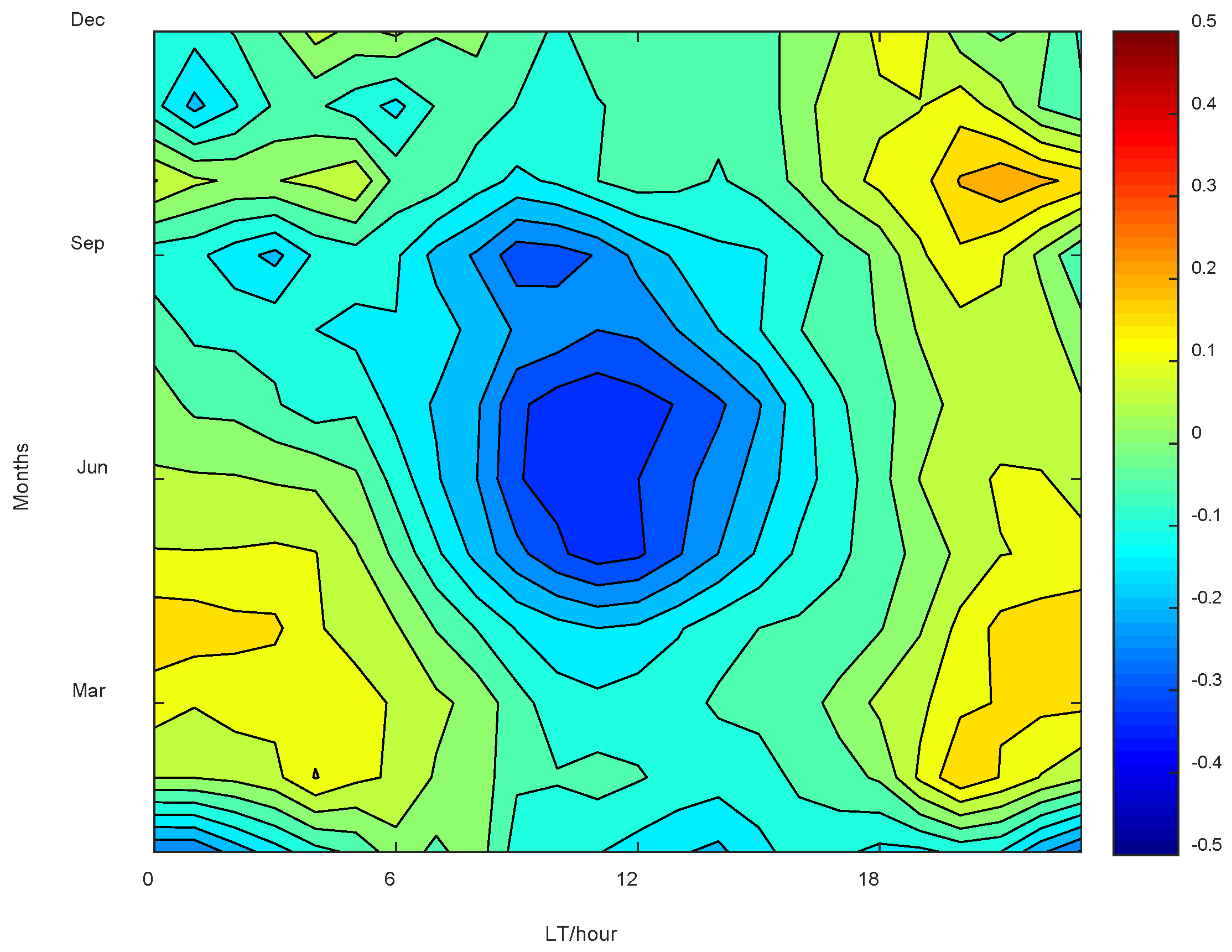
The east-west TEC longitudinal difference index Re/w over East Asia is negative at noon and positive at evening-night in the high solar activity year, consistent with local time variations of Re/w in previous studies.
(2)
The longitudinal difference in daytime TEC is most evident in summer, less in autumn and least in spring and winter, while the nighttime difference is most obvious in equinox, followed by summer and winter during the pre-midnight period. It is noteworthy that the longitudinal difference after midnight is most significant in spring, and it is weak in autumn months, indicating a semi-annual asymmetry during this period. The seasonal features are basically consistent with the previous studies of longitudinal differences in NmF2 in East Asia.
(3)
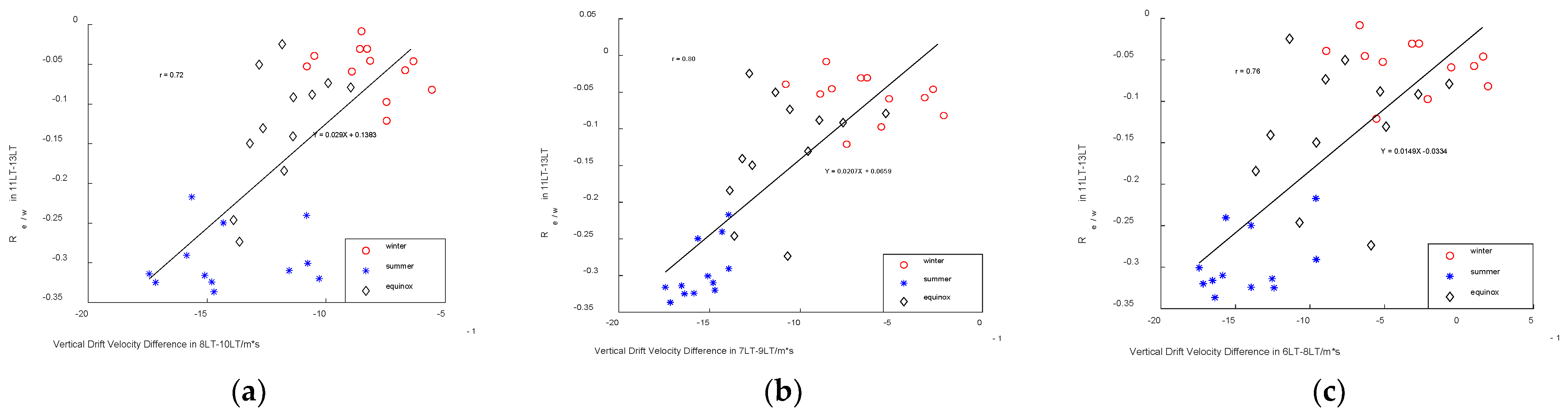
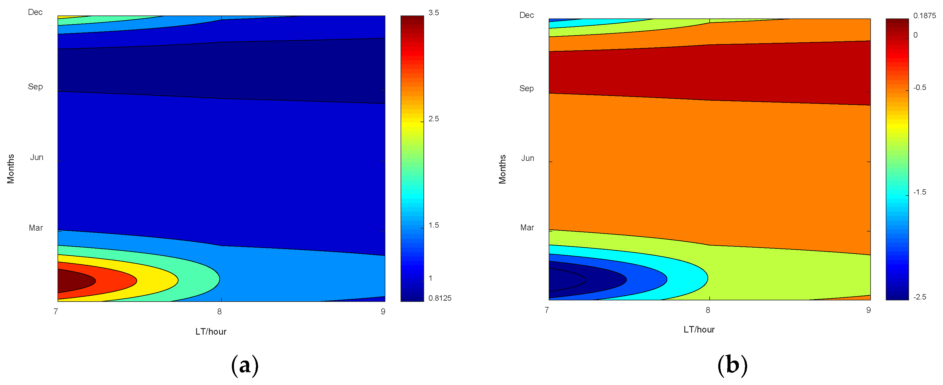
The TEC longitudinal difference around noon in high solar activity year is mainly caused by the zonal wind-declination mechanism proposed by previous studies. Moreover, a 4-h time delay seems to be an optimal result for the vertical drift velocity to cause the longitudinal TEC difference during pre-noon hours, consistent with the result of previous modeling studies.
(4)
The solar activity does not seem to affect both positive and negative Re/w simultaneously, which is consistent with previous studies for the electron density longitudinal difference in East Asian and North American mid-latitudes.
Additionally, we obtained some novel findings that shed an interesting light on the TEC longitudinal difference in this area:
(1)
In addition to the vertical drift velocity difference caused by the geomagnetic configuration-neutral wind mechanism, the local electron density is also an important factor influencing the TEC longitudinal difference at high solar activity year night.
(2)
There was about a 3 h time delay between the TEC longitudinal variations and the uplifting electron flux at high solar activity year night. The difference in time delay for daytime (~4 h) and nighttime (~3 h) might result from the higher electron density, which could result in a stronger ion-drag effect during the daytime.
(3)
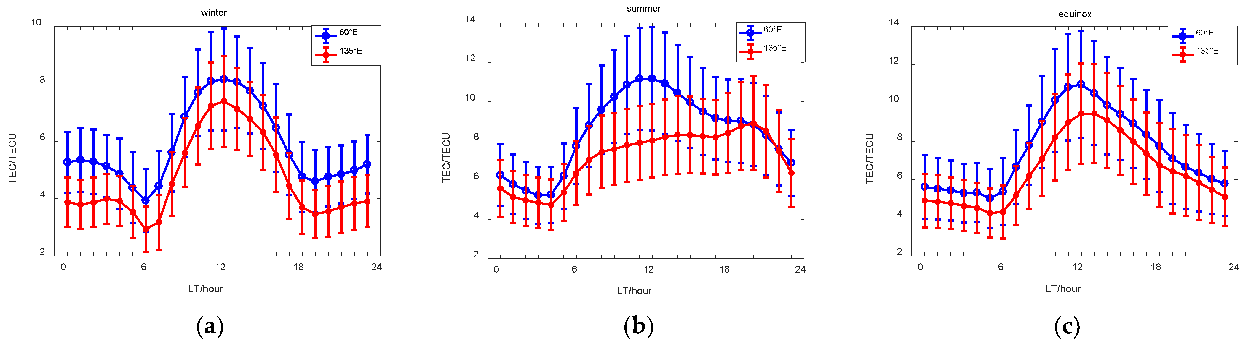
The western TEC is greater than the eastern TEC during most periods of the low solar activity years except in summer evening, and the positive summer evening Re/w might have a relationship with the midlatitude summer nighttime anomaly (MSNA) in the northeast region of East Asia.
(4)
The ionospheric nighttime enhancement seems also could modulate the Re/w, especially in the low solar activity year winter when this phenomenon occurred most frequently.
(5)
The Re/w in the low solar activity year nighttime could not explain only by the geomagnetic configuration-neutral wind mechanism and local electron density, and there are systematic differences in TEC diurnal variation between east and west of East Asia in winter and equinox.
This paper presents a statistical analysis of the diurnal, seasonal and solar cycle variation in the TEC longitudinal difference in midlatitudes of East Asia. The results can contribute to the understanding of ionosphere-thermosphere coupling, and it can be applicable to improving the ionospheric model. In future work, more observations and modeling are needed to study other possible physical drivers of the TEC longitudinal difference in midlatitudes of East Asia, especially the longitudinal differences in low solar activity years.

Author Contributions

Conceptualization, X.S., J.F., Y.Z. (Yuqiang Zhang) and Z.W.; methodology, Z.W. and C.Z.; investigation, J.F., T.X., F.Z. and C.Z.; validation, Y.Z. (Yufeng Zhou); formal analysis, X.S. and Y.Z. (Yuqiang Zhang); resources, Z.Z. and Z.D.; visualization, N.X.; funding acquisition, Y.L. and T.X. All authors have read and agreed to the published version of the manuscript.

Funding

This work was supported by the National Key Laboratory of Electromagnetic Environment (Grant No. 20200101) and Natural Basic Scientific Research Program of China (Program No. JCKY2021210C614240302).

Data Availability Statement

The use of COSMIC IRO data was provided by CDAAC (COSMIC Data Analysis of Archive Center, http://cdaac-www.cosmic.ucar.edu/cdaac/products.htm, accessed on 28 September 2022). The use of TEC data was provided by CODE (Center for Orbit Determination in Europe, ftp://ftp.unibe.ch/aiub/CODE/, accessed on 28 September 2022). The use of Ap data was provided by WDC (World Data Center, http://wdc.kugi.kyoto-u.ac.jp/, accessed on 28 September 2022). The use of F10.7 data was provided by NOAA (ftp://ftp.swpc.noaa.gov/pub/indices/old_indices/, accessed on 28 September 2022).

Acknowledgments

We acknowledge the use of ionosonde data provided by the GIRO (Global Ionospheric Radio Observation) database (http://umlcar.uml.edu/DIDbase, 28 September 2022), GPS data provided by the UNAVCO database (University NAVSTAR Consortium) (http://www.unavco.org/, 28 September 2022), Dst data provided by WDC (http://wdc.kugi.kyoto-u.ac.jp/, 28 September 2022) and F10.7 data provided by NOAA (ftp://ftp.swpc.noaa.gov/pub/indices/old_indices/, 28 September 2022).

Conflicts of Interest

The authors declare no conflict of interest.

Appendix A

Figure A1. The difference in east (60°E, 47.5°N) and west (135°E, 47.5°N) vertical drift velocity at (a) 250 km, (b) 300 km and (c) 350 km heights calculated by the HWM-14 model and IGRF-2020 model.
Remotesensing 14 05412 g0a1
Table A1. Statistics of the difference in the east region (125°E–145°E, 45°N–50°N)-west region (50°E–70°E, 45°N–50°N) uplifting electron flux obtained from the COSMIC NmF2 data and vertical drift velocity calculated from the HWM-14 model. he red color represents the NmF2 in winter, the blue color represents the NmF2 in summer, the yellow color represents the NmF2 in equinox.
LTNmF2 in 60°E, 47.5°NVz in 60°E, 47.5°NUplifting Electron Flux Per Second in 60°E, 47.5°NNmF2 in 135°E, 47.5°NVz in 135°E, 47.5°NUplifting Electron Flux per Second in 135°E, 47.5°NUplifting Electron Flux Difference Per SecondRe/w in LT + 3
UnitHour1010 el/m3m/s1010 el/m21010 el/m3m/s1010 el/m21010 el/m2
18.0030.48−26.12−796.0936.79−11.26−414.34381.750.06
19.0025.44−21.29−541.6027.37−3.44−94.27447.330.03
20.0014.42−16.76−241.6122.212.9665.80307.40−0.02
winter21.0015.82−13.30−210.4114.996.69100.29310.70−0.07
22.0011.37−10.73−121.9711.307.9489.73211.70−0.09
23.0019.37−8.09−156.6117.688.23145.57302.18−0.11
24.0019.00−4.30−81.6516.789.47158.87240.52−0.07
18.0056.320.3016.9455.0011.46630.06613.130.08
19.0062.05−0.08−4.7858.7213.62799.67804.440.09
20.0058.690.2715.8564.4713.95899.09883.240.09
summer21.0056.143.11174.4964.7114.37929.70755.200.07
22.0055.629.16509.6969.2616.831165.89656.200.04
23.0040.8817.74725.1453.8822.281200.52475.370.02
24.0044.1527.011192.4653.1330.071597.46404.990.02
18.0075.25−12.17−915.9071.272.94209.521125.420.15
19.0069.21−8.70−602.0677.6910.19791.731393.800.17
20.0057.32−5.59−320.6771.2815.021070.941391.610.15
equinox21.0049.91−3.04−151.7860.5417.121036.671188.450.12
22.0035.09−0.66−23.1652.8317.70935.25958.410.08
23.0028.122.1861.2434.4018.77645.54584.300.06
24.0028.635.85167.4243.6221.83952.33784.910.05
Table A2. Statistics of the difference in the east region (125°E–145°E, 45°N–50°N)-west region (50°E–70°E, 45°N–50°N) uplifting electron flux in spring and autumn in the high solar activity year.
LTNmF2 in 60°EVz in 60°E, 47.5°NUplifting Electron Flux Per Second in 60°E, 47.5°NNmF2 in 135°EVz in 135°E, 47.5°NUplifting Electron Flux Difference Per SecondUplifting Electron Flux Difference Per SecondRe/w in LT + 3
UnitHour1010 el/m3m/s1010 el/m21010 el/m3m/s1010 el/m21010 el/m2
21.0058.07−1.63−94.7763.3515.40975.351070.110.13
spring22.0039.401.2047.2883.1715.731308.291261.010.12
23.0031.213.90121.7137.7915.03567.88446.170.11
24.0030.557.44227.2055.2015.49855.04627.840.12
21.0036.342.79101.3752.0616.01833.58732.210.05
autumn22.0023.217.48173.5931.0218.07560.64387.060.00
23.0025.6313.93356.8521.2321.68460.36103.50−0.03
24.0018.4321.41394.5930.2927.28826.44431.84−0.05

References

  1. Appleton, E.V. Two Anomalies in the Ionosphere. Nature 1946, 157, 691. [Google Scholar] [CrossRef]
  2. Moffett, R.J.; Hanson, W.B. Effect of Ionization Transport on the Equatorial F-Region. Nature 1965, 206, 705–706. [Google Scholar] [CrossRef]
  3. Huang, Y.-N.; Cheng, K. Solar cycle variations of the equatorial ionospheric anomaly in total electron content in the Asian region. J. Geophys. Res. Space Res. 1996, 101, 24513–24520. [Google Scholar] [CrossRef]
  4. Zhao, B.; Wan, W.; Liu, L.; Ren, Z. Characteristics of the ionospheric total electron content of the equatorial ionization anomaly in the Asian-Australian region during 1996–2004. Ann. Geophys. 2009, 27, 3861–3873. [Google Scholar] [CrossRef] [Green Version]
  5. Balan, N.; Liu, L.; Le, H. A brief review of equatorial ionization anomaly and ionospheric irregularities. Earth. Planet. Phys. 2018, 2, 257–275. [Google Scholar] [CrossRef]
  6. Muldrew, D.B. F-layer ionization troughs deduced from Alouette data. J. Geophys. Res. 1965, 70, 2635–2650. [Google Scholar] [CrossRef]
  7. Sharp, G.W. Midlatitude trough in the night ionosphere. J. Geophys. Res. 1966, 71, 1345–1356. [Google Scholar] [CrossRef]
  8. Rodger, A. The Mid-Latitude Trough—Revisited. In Washington DC American Geophysical Union Geophysical Monograph Series; AGU: Washington, DC, USA, 2008; Volume 181, pp. 25–33. [Google Scholar]
  9. Zou, S.; Moldwin, M.B.; Coster, A.; Lyons, L.R.; Nicolls, M.J. GPS TEC observations of dynamics of the mid-latitude trough during substorms. Geophys. Res. Lett. 2011, 38, L14109. [Google Scholar] [CrossRef] [Green Version]
  10. He, S.C.; Zhang, D.H.; Hao, Y.Q.; Xiao, Z. Statistical study on the occurrence of the ionospheric mid-latitude trough and the variation of trough minimum location over northern hemisphere. Chinese J. Geophys. 2020, 63, 31–64. [Google Scholar]
  11. Sagawa, E.; Immel, T.J.; Frey, H.U.; Mende, S.B. Longitudinal structure of the equatorial anomaly in the nighttime ionosphere observed by IMAGE/FUV. J. Geophys. Res. 2005, 110, A11302. [Google Scholar]
  12. England, S.L.; Immel, T.J.; Sagawa, E.; Henderson, S.B.; Hagan, M.E.; Mende, S.B.; Frey, H.U.; Swenson, C.M.; Paxton, L.J. Effect of atmospheric tides on the morphology of the quiet time, postsunset equatorial ionospheric anomaly. J. Geophys. Res. 2006, 111, A10S19. [Google Scholar] [CrossRef]
  13. Lin, C.H.; Hsiao, C.C.; Liu, J.Y.; Liu, C.H. Longitudinal structure of the equatorial ionosphere: Time evolution of the four-peaked EIA structure. J. Geophys. Res. Space Res. 2007, 112, A12305. [Google Scholar] [CrossRef]
  14. Wan, W.; Liu, L.; Pi, X.; Zhang, M.L.; Ning, B.; Xiong, J.; Ding, F. Wavenumber-4 patterns of the total electron content over the low latitude ionosphere. Geophys. Res. Lett. 2008, 35, L12104. [Google Scholar] [CrossRef]
  15. Immel, T.J.; Sagawa, E.; England, S.L.; Henderson, S.B.; Hagan, M.E.; Mende, S.B.; Frey, H.U.; Swenson, C.M.; Paxton, L.J. Control of equatorial ionospheric morphology by atmospheric tides. Geophys. Res. Lett. 2006, 33, L15108. [Google Scholar] [CrossRef]
  16. England, S.L.; Maus, S.; Immel, T.J.; Mende, S.B. Longitudinal variation of the E-region electric fields caused by atmospheric tides. Geophys. Res. Lett. 2006, 33, L21105. [Google Scholar] [CrossRef] [Green Version]
  17. Hagan, M.E.; Maute, A.; Roble, R.G.; Richmond, A.D.; Immel, T.J.; England, S.L. Connections between deep tropical clouds and the Earth’s ionosphere. Geophys. Res. Lett. 2007, 34, L20109. [Google Scholar] [CrossRef] [Green Version]
  18. Ren, Z.; Wan, W.; Xiong, J.; Liu, L. Simulated wave number 4 structure in equatorial F-region vertical plasma drifts. J. Geophys. Res. Atmos. 2010, 115, A05301. [Google Scholar] [CrossRef]
  19. Zou, L.; Rishbeth, H.; Müller-Wodarg, I.; Aylward, A.D.; Millward, G.H.; Fuller-Rowell, T.J.; Idenden, D.W.; Moffett, R.J. Annual and semiannual variations in the ionospheric F2-layer: I. Modelling. Ann. Geophys. 2000, 18, 927–944. [Google Scholar] [CrossRef]
  20. Rishbeth, H.; Müller-Wodarg, I.; Zou, L.; Fuller-Rowell, T.J.; Aylward, A.D. Annual and semiannual variations in the ionospheric F2-layer: II. Physical discussion. Ann. Geophys. 2000, 18, 945–956. [Google Scholar] [CrossRef]
  21. Liu, H.; Thampi, S.V.; Yamamoto, M. Phase reversal of the diurnal cycle in the midlatitude ionosphere. J. Geophys. Res. Space Res. 2010, 115, A01305. [Google Scholar] [CrossRef] [Green Version]
  22. Liu, L.; Le, H.; Chen, Y.; He, M.; Wan, W.; Yue, X. Features of the middle- and low-latitude ionosphere during solar minimum as revealed from COSMIC radio occultation measurements. J. Geophys. Res. Space Res. 2011, 116, A09307. [Google Scholar] [CrossRef]
  23. Zhang, S.-R.; Foster, J.C.; Coster, A.J.; Erickson, P.J. East-West Coast differences in total electron content over the continental US. Geophys. Res. Lett. 2011, 38, 542–553. [Google Scholar] [CrossRef]
  24. Zhang, S.-R.; Foster, J.C.; Holt, J.M.; Erickson, P.J.; Coster, A.J. Magnetic declination and zonal wind effects on longitudinal differences of ionospheric electron density at midlatitudes. J. Geophys. Res. Space Res. 2012, 117, A08329. [Google Scholar] [CrossRef] [Green Version]
  25. Zhang, S.; Coster, A.J.; Holt, J.M.; Foster, J.C.; Erickson, P. Ionospheric longitudinal variations at midlatitudes: Incoherent scatter radar observation at Millstone Hill. Sci. China Technol. Sci. 2012, 55, 1153–1160. [Google Scholar] [CrossRef] [Green Version]
  26. Zhang, S.-R.; Chen, Z.; Coster, A.J.; Erickson, P.J.; Foster, J.C. Ionospheric symmetry caused by geomagnetic declination over North America. Geophys. Res. Lett. 2013, 40, 5350–5354. [Google Scholar] [CrossRef] [Green Version]
  27. Zhao, B.; Wang, M.; Wang, Y.; Ren, Z.; Yue, X.; Zhu, J.; Wan, W.; Ning, B.; Liu, J.; Xiong, B. East-west differences in F-region electron density at midlatitude: Evidence from the Far East region. J. Geophys. Res. Space Res. 2013, 118, 542–553. [Google Scholar] [CrossRef]
  28. Xu, J.S.; Li, X.J.; Liu, Y.W.; Jing, M. TEC differences for the mid-latitude ionosphere in both sides of the longitudes with zero declination. Adv. Space Res. 2014, 54, 883–895. [Google Scholar] [CrossRef]
  29. Wang, H.; Liu, D. Tidal spectrum analysis of electron density and plasma vertical velocity at mid-latitudes. Chin. Sci. Bull. 2015, 60, 3239–3250. [Google Scholar]
  30. Wang, H.; Ridley, A.J.; Zhu, J. Theoretical study of zonal differences of electron density at midlatitudes with GITM simulation. J. Geophys. Res. Space Res. 2015, 120, 2951–2966. [Google Scholar] [CrossRef]
  31. Wang, H.; Liu, D.; Zhang, J. Vertical structure of longitudinal differences in electron densities at mid-latitudes. Sci. Bull. 2016, 61, 252–262. [Google Scholar] [CrossRef] [Green Version]
  32. Wang, H.; Zhang, K. Longitudinal structure in electron density at mid-latitudes: Upward-propagating tidal effects. Earth Planet Space 2017, 69, 11. [Google Scholar] [CrossRef] [Green Version]
  33. Ren, Z.; Zhao, B.; Wan, W.; Liu, L.; Li, X.; Yu, T. Simulated east-west differences in F-region peak electron density at Far East mid-latitude region. Earth Planet Space 2020, 72, 50. [Google Scholar] [CrossRef] [Green Version]
  34. Luan, X.; Dou, X. Seasonal dependence of the longitudinal variations of nighttime ionospheric electron density and equivalent winds at southern midlatitudes. Ann. Geophys. 2013, 31, 1699–1708. [Google Scholar] [CrossRef]
  35. Tsagouri, I.; Goncharenko, L.; Shim, J.S.; Belehaki, A.; Buresova, D.; Kuznetsova, M.M. Assessment of current capabilities in modeling the ionospheric climatology for space weather applications: foF2 and hmF2. Space Weather 2018, 16, 1930–1945. [Google Scholar] [CrossRef] [Green Version]
  36. Yao, X.; Zhao, B.; Liu, L.; Wan, W. Comparison of ionospheric total electron content over North America and East Asia with EOF analysis. Chin. J. Space Sci. 2015, 35, 556–565. [Google Scholar]
  37. Shim, J.S.; Jee, G.; Scherliess, L. Climatology of plasmaspheric total electron content obtained from Jason 1 satellite. J. Geophys. Res. Space Phys. 2017, 122, 1611–1623. [Google Scholar] [CrossRef] [Green Version]
  38. Zhong, J.; Lei, J.; Wang, W.; Burns, A.G.; Yue, X.; Dou, X. Longitudinal variations of topside ionospheric and plasmaspheric TEC. J. Geophys. Res. Space Phys. 2017, 122, 6737–6760. [Google Scholar] [CrossRef]
  39. Jin, S.; van Dam, T.; Wdowinski, S. Observing and understanding the Earth system variations from space geodesy. J. Geodyn. 2013, 72, 1–10. [Google Scholar] [CrossRef] [Green Version]
  40. Jin, S.; Jin, R.; Li, D. Assessment of BeiDou differential code bias variations from multi-GNSS network observations. Ann. Geophys. 2016, 34, 259–269. [Google Scholar] [CrossRef] [Green Version]
  41. Dach, R.; Brockmann, E.; Schaer, S.; Beutler, G.; Meindl, M.; Prange, L.; Bock, H.; Jäggi, A.; Ostini, L. GNSS processing at CODE: Status report. J. Geodesy. 2009, 83, 353–365. [Google Scholar] [CrossRef] [Green Version]
  42. Feltens, J. The International GPS Service (IGS) Ionosphere Working Group. Adv. Space Res. 2003, 31, 635–644. [Google Scholar] [CrossRef]
  43. Schaer, S. Mapping and Predicting the Earth’s Ionosphere Using the Global Positioning System; Geod Geophys.arb.schweiz; Institut für Geodäsie und Photogrammetrie, Eidg. Technische Hochschule Zürich: Zürich, Switzerland, 1999. [Google Scholar]
  44. Hernández-Pajares, M.; Juan, J.M.; Sanz, J.; Orus, R.; Garcia-Rigo, A.; Feltens, J.; Komjathy, A.; Schaer, S.C.; Krankowski, A. The IGS VTEC maps: A reliable source of ionospheric information since 1998. J. Geodesy. 2009, 83, 263–275. [Google Scholar] [CrossRef]
  45. Lei, J.; Syndergaard, S.; Burns, A.G.; Solomon, S.C.; Wang, W.; Zeng, Z.; Roble, R.G.; Wu, Q.; Kuo, Y.-H.; Holt, J.M.; et al. Comparison of COSMIC ionospheric measurements with ground-based observations and model predictions: Preliminary results. J. Geophys. Res. Space Phys. 2007, 112, A07308. [Google Scholar] [CrossRef]
  46. Kelley, M.C.; Wong, V.K.; Aponte, N.; Coker, C.; Mannucci, A.J.; Komjathy, A. Comparison of COSMIC occultation-based electron density profiles and TIP observations with Arecibo incoherent scatter radar data. Radio Sci. 2009, 44, RS4011. [Google Scholar] [CrossRef]
  47. Sun, L.; Zhao, B.; Yue, X.; Mao, T. Comparison between ionospheric character parameters retrieved from FORMOSAT3 measurement and ionosonde observation over China. Chin. J. Geophys. 2014, 57, 3625–3632. [Google Scholar]
  48. Hedin, A.E.; Biondi, M.A.; Burnside, R.G.; Hernandez, G.; Johnson, R.M. Revised Global Model of Thermosphere Winds Using Satellite and Ground-Based Observations. J. Geophys. Res. Space Phys. 1991, 96, 7657–7688. [Google Scholar] [CrossRef] [Green Version]
  49. Drob, D.P.; Emmert, J.T.; Crowley, G.; Picone, J.M.; Shepherd, G.G.; Skinner, W.; Hays, P.; Niciejewski, R.J.; Larsen, M.; She, C.Y.; et al. An empirical model of the Earth’s horizontal wind fields: HWM07. J. Geophys. Res. Space Res. 2008, 113, A12304. [Google Scholar] [CrossRef] [Green Version]
  50. Emmert, J.T.; Drob, D.P.; Shepherd, G.G.; Hernandez, G.; Jarvis, M.J.; Meriwether, J.W.; Niciejewski, R.J.; Sipler, D.P.; Tepley, C.A. DWM07 global empirical model of upper thermospheric storm-induced disturbance winds. J. Geophys. Res. Space Res. 2008, 113, A11319. [Google Scholar] [CrossRef]
  51. Drob, D.P.; Emmert, J.T.; Meriwether, J.W.; Makela, J.J.; Doornbos, E.; Conde, M.; Hernandez, G.; Noto, J.; Zawdie, K.A.; McDonald, S.E.; et al. An update to the Horizontal Wind Model (HWM): The quiet time thermosphere. Earth Space Sci. 2015, 2, 301–319. [Google Scholar] [CrossRef]
  52. Bellchambers, W.H.; Piggott, W.R. Ionospheric Measurements made at Halley Bay. Nature 1958, 182, 1596–1597. [Google Scholar] [CrossRef]
  53. Penndorf, R. The Average Ionospheric Conditions Over the Antarctic. In Geomagnetism and Aeronomy: Studies in the Ionosphere, Geomagnetism and Atmospheric Radio Noise; Waynick, A.H., Ed.; Wiley: Hoboken, NJ, USA, 1965. [Google Scholar] [CrossRef]
  54. Horvath, I.; Essex, E.A. The Weddell sea anomaly observed with the Topex satellite data. J. Atomos. Sol. Terr. Phys. 2003, 65, 693–706. [Google Scholar] [CrossRef]
  55. He, M.; Liu, L.; Wan, W.; Ning, B.; Zhao, B.; Wen, J.; Yue, X.; Le, H. A study of the Weddell Sea Anomaly observed by FORMOSAT-3/COSMIC. J. Geophys. Res. Space Res. 2009, 114, A12309. [Google Scholar] [CrossRef] [Green Version]
  56. Lin, C.H.; Liu, J.Y.; Cheng, C.Z.; Chen, C.H.; Liu, C.H.; Wang, W.; Burns, A.G.; Lei, J. Three-dimensional ionospheric electron density structure of the Weddell Sea Anomaly. J. Geophys. Res. Space Res. 2009, 114, A02312. [Google Scholar] [CrossRef] [Green Version]
  57. Lin, C.H.; Liu, C.H.; Liu, J.Y.; Chen, C.H.; Burns, A.G.; Wang, W. Midlatitude summer nighttime anomaly of the ionospheric electron density observed by FORMOSAT-3/COSMIC. J. Geophys. Res. Space Res. 2010, 115, A03308. [Google Scholar] [CrossRef]
  58. Chen, Y.; Liu, L.; Le, H.; Wan, W.; Zhang, H. The global distribution of the dusk-to-nighttime enhancement of summer NmF2 at solar minimum. J. Geophys. Res. Space Res. 2016, 121, 7914–7922. [Google Scholar] [CrossRef]
  59. Richards, P.G.; Meier, R.R.; Chen, S.; Dandenault, P. Investigation of the Causes of the Longitudinal and Solar Cycle Variation of the Electron Density in the Bering Sea and Weddell Sea Anomalies. J. Geophys. Res. Space Res. 2018, 123, 7825–7842. [Google Scholar] [CrossRef]
  60. Balan, N.; Rao, P.B. Latitudinal variations of nighttime enhancements in total electron content. J. Geophys. Res. 1987, 92, 3436–3440. [Google Scholar] [CrossRef]
  61. Farelo, A.F.; Herraiz, M.; Mikhailov, A.V. Global morphology of night-time NmF2 enhancements. Ann. Geophys. 2002, 20, 1795–1806. [Google Scholar] [CrossRef] [Green Version]
  62. Jakowski, N.; Jungstand, A.; Lois, L.; Lazo, B. Night-time enhancements of the F2-layer ionization over Havana, Cuba. J. Atmos. Terr. Phys. 1991, 53, 1131–1138. [Google Scholar] [CrossRef]
  63. Jakowski, N.; Hoque, M.M.; Kriegel, M.; Patidar, V. The persistence of the NWA effect during the low solar activity period 2007–2009. J. Geophys. Res. Space Res. 2015, 120, 9148–9160. [Google Scholar] [CrossRef]
  64. Chen, Y.; Liu, L.; Le, H.; Wan, W.; Zhang, H. NmF2 enhancement during ionospheric F2 region nighttime: A statistical analysis based on COSMIC observations during the 2007–2009 solar minimum. J. Geophys. Res. Space Res. 2016, 120, 10083–10095. [Google Scholar] [CrossRef]
  65. Li, W.; Chen, Y.; Liu, L.; Le, H.; Huang, C. A Statistical Study on the Winter Ionospheric Nighttime Enhancement at Middle Latitudes in the Northern Hemisphere. J. Geophys. Res. Space Res. 2020, 125, e2020JA027950. [Google Scholar] [CrossRef]
  66. Bailey, G.J.; Sellek, R.; Balan, N. The effect of interhemispheric coupling on nighttime enhancements in ionospheric total electron content during winter at solar minimum. Ann. Geophys. 1991, 9, 738–747. [Google Scholar]
  67. Dabas, R.S.; Kersley, L. Study of mid-latitude nighttime enhancement in F-region electron density using tomographic images over the UK. Ann. Geophys. 2003, 21, 2323–2328. [Google Scholar] [CrossRef] [Green Version]
  68. Jakowski, N.; Förster, M. About the nature of the Night-time Winter Anomaly effect (NWA) in the F-region of the ionosphere. Planet. Space Sci. 1995, 43, 603–612. [Google Scholar] [CrossRef]
  69. Li, Q.; Hao, Y.; Zhang, D.; Xiao, Z. Nighttime Enhancements in the Midlatitude Ionosphere and Their Relation to the Plasmasphere. J. Geophys. Res. Space Res. 2018, 123, 7686–7696. [Google Scholar] [CrossRef]
Figure 1. The solar activity index F10.7 during the years 2015–2020.
Remotesensing 14 05412 g001
Figure 2. Averaged TEC in the East Asian middle latitude (45°N–50°N) on 10 June 2015.
Remotesensing 14 05412 g002
Figure 3. Diurnal variation of TEC longitude difference index Re/w in East Asia in 2015, a high solar activity year.
Remotesensing 14 05412 g003
Figure 4. Diurnal variation of TEC longitude difference index Re/w in East Asia in 2018 and 2019, two low solar activity years.
Remotesensing 14 05412 g004
Figure 5. Local time variations of the east-to-west differential index Re/w in spring, summer, autumn and winter in high and low solar activity years.
Remotesensing 14 05412 g005
Figure 6. (a) Vertical drift velocity in 60°E, 47.5°N; (b) Vertical drift velocity in 135°E, 47.5°N; (c) Vertical drift velocity difference between them.
Remotesensing 14 05412 g006
Figure 7. (a) Correlation between the TEC longitudinal differences index Re/w in 11LT–13LT and the vertical drift velocity difference in 8LT–10LT in high solar activity years. (b) Correlation between the TEC longitudinal difference index Re/w in 11LT–13LT and the vertical drift velocity difference in 7LT–9LT in high solar activity years. (c) Correlation between the TEC longitudinal difference index Re/w in 11LT–13LT and the vertical drift velocity difference in 6LT–8LT in high solar activity years.
Remotesensing 14 05412 g007
Figure 8. (a) The ratio of vertical drift velocity difference Δ ( sin I cos I U sin D ) caused by zonal wind to the total drift velocity difference Δ V z (b) The ratio of vertical drift velocity difference Δ ( sin I cos I V cos D ) caused by horizontal wind to the total drift velocity difference Δ V z .
Remotesensing 14 05412 g008
Figure 9. (a) Correlation between the TEC longitudinal difference index Re/w in 21LT–03LT and the difference of uplifting electron flux per second in 19LT–01LT in high solar activity years. (b) Correlation between the TEC longitudinal difference index Re/w in 21LT–03LT and the difference of uplifting electron flux per second in 18LT–24LT in high solar activity years. (c) Correlation between the TEC longitudinal difference index Re/w in 21LT–03LT and difference of uplifting electron flux per second in 17LT–23LT in high solar activity years.
Remotesensing 14 05412 g009
Figure 10. (a) Correlation between the TEC longitudinal difference index Re/w in 11LT–13LT and the corresponding vertical drift velocity difference in 8LT–10LT in low solar activity years. (b) Correlation between the TEC longitudinal difference index Re/w in 11LT–13LT and the corresponding vertical drift velocity difference in 7LT–9LT in low solar activity years. (c) Correlation between the TEC longitudinal difference index Re/w in 11LT–13LT and the corresponding vertical drift velocity difference in 6LT–8LT in low solar activity years.
Remotesensing 14 05412 g010
Figure 11. The diurnal variations of mean and standard deviation of TEC in the East Asian midlatitudes (60°E, 45°N–50°N; 135°E, 45°N–50°N) in (a) summer, (b) winter and (c) equinox in the geomagnetic quiet condition.
Remotesensing 14 05412 g011
Table 1. Geographic longitude, latitude and magnetic declination/inclination of the chosen GIMs grid point.
Area Longitude/°Latitude/°Declination/°Inclination/°
Grid Point 113545−9.5760.91
EastGrid Point 213547.5−10.2263.37
Grid Point 313550−10.8565.71
Grid Point 160456.9664.3
WestGrid Point 26047.58.0166.52
Grid Point 360509.1668.58
Publisher’s Note: MDPI stays neutral with regard to jurisdictional claims in published maps and institutional affiliations.

