Article

Contrasting Mesoscale Convective System Features of Two Successive Warm-Sector Rainfall Episodes in Southeastern China: A Satellite Perspective

1
Xiamen Key Laboratory of Straits Meteorology, Xiamen Meteorological Bureau, Xiamen 361012, China
2
State Key Laboratory of Marine Environmental Science, College of Ocean and Earth Sciences, Xiamen University, Xiamen 361102, China
*
Author to whom correspondence should be addressed.
Remote Sens. 2022, 14(21), 5434; https://doi.org/10.3390/rs14215434
Submission received: 3 September 2022 / Revised: 21 October 2022 / Accepted: 24 October 2022 / Published: 28 October 2022

Abstract

:
Based on Himawari-8 satellite observations, the mesoscale convective system (MCS) behaviors of two successive but distinct warm-sector rainfall episodes (EP1 and EP2) on 6–7 May 2018 over southeastern China were compared, with the latter episode being a record-breaking rainfall event. Results showed that MCSs played a dominant role in EP2, but not in EP1, by contributing over 80% of the extreme rainfall total and all the 10-min rainfalls over 20 mm. MCS occurrences were more frequent in EP2 than EP1, especially in the coastal rainfall hotspots, along with more frequent merging processes. Overall, the MCS samples in EP2 were larger in size, more intense, and moved slower and more in parallel to their orientation, which facilitated local rainfall accumulation. Two new indices are proposed—the overlap index (OLI) and merging potential index (MPI)—to evaluate two MCS processes vital for rainfall production: the repeated passage of an individual MCS over given areas and the merging between MCSs, respectively. Both OLI and MPI in EP2 were significantly larger than in EP1, which tended to produce larger maximum rainfall amount and stronger 10-min rain rates in the following hour. These results demonstrate the potential value of satellite-based MCS information for heavy rainfall nowcasting, which is particularly significant for warm-sector rainfall with its limited predictability.

1. Introduction

Located in the East Asian monsoon region, South China witnesses abundant rainfall during the pre-summer rainy season (April–June), which contributes approximately half of the annual precipitation amount [1]. Pre-summer rainfalls commonly occur either near synoptic fronts or in the warm sector about 200–300 km ahead of a front (sometimes even without an associated front) [1,2], termed frontal rainfalls and warm-sector rainfalls. Climatological studies show that warm-sector and frontal rainfalls are mainly concentrated in coastal and inland areas, respectively [3,4]. Without strong synoptic forcing, warm-sector rainfalls are often more associated with multiple complex factors including moist and unstable low-level jets [5,6], coastal topography [7,8], land–sea contrast [3,9], cold pools [8,10], and urban effects [11,12]. Consequently, warm-sector rainfalls are often characterized by sudden occurrence and high precipitation intensity [1,3], but with low predictability [13,14], thereby frequently causing destructive impacts on the populated urban agglomerations of South China. Notably, although the differences between frontal and warm-sector rainfall have received considerable attention, the distinct features in different warm-sector rainfall events themselves are less well documented, which is the motivation behind the present study.
Mesoscale convective systems (MCSs) are recognized as a major rainfall producer [15,16]. In most rainy areas of the tropics and subtropics, including South China, MCSs contribute over half of the rainfall total (e.g., [17,18]). Meanwhile, MCSs show great potential to produce extreme rainfall events (e.g., [19,20]). Climatological results show that the rainfall contributions from MCSs can vary seasonally, diurnally, and regionally with distinct synoptic environments (e.g., [16,21,22]). In South China, MCSs have also been found to be responsible for many warm-sector heavy rainfall cases [1,23,24]. However, a clear quantification of the MCS contribution to individual instances of warm-sector rainfall and its variation between cases have remained elusive.
The MCS–rainfall relationship is closely related to MCS features, including morphology, intensity, duration, and motion (e.g., [16,17,18]). Generally speaking, slow-moving MCSs with large size and intense convection tend to have a long lifetime and produce long-duration local rainfall and even extreme rainfall events (e.g., [18,19,25,26]). Moreover, linear (elongated) MCSs are known to be more conducive than nonlinear MCSs to producing heavy and even extreme precipitation, especially those with a training line/adjoining stratiform and back-building/quasi-stationary organization mode (e.g., [26,27,28]).
In South China, Li, et al. [29] examined 92 MCSs associated with warm-sector heavy rainfall and found the linear modes accounted for 60% of them. Chen, et al. [30] examined 98 quasi-linear MCSs over South China during the pre-summer rainy seasons and found that the mode of multiple convective bands with stratiform precipitation mainly appeared near the coastline and had a long lifespan and slow moving speed, which caused some warm-sector extreme rainfall cases [10,31,32]. Given the limited predictability of warm-sector heavy rainfall in numerical models, synthesizing important MCS features in real-time observations can help to assess the rainfall production potential and thus improve the prediction of rainfall.
This paper contrasts the MCS contributions and features between two warm-sector rainfall episodes in southeastern China. These two episodes occurred in succession on 6–7 May 2018 but had distinct rainfall totals and intensities. The latter rainfall episode was an extreme record-breaking rainfall event that caused severe urban inundation and socio-economic losses [33,34]. The former rainfall episode was noticed since it happened just a few hours before the latter rainfall episode, in a similar warm-sector environment but with moderate rainfall amount and intensity. Compared with the general features of warm-sector MCSs in South China examined in Li, et al. [29], MCSs in both episodes similarly preferred a quasi-linear organizational mode and eastward propagation; the MCSs in the latter (former) episode produced overall heavier (lighter) rainfall than the climatological value. Comparison between such back-to-back episodes will help in improving knowledge on the different roles of MCSs in warm-sector rainfalls during a short time span. The MCS features were obtained based on the observations from Himawari-8, a state-of-the-art geostationary satellite. Satellite observations have been widely used in investigating MCS properties across the globe (e.g., [15,35,36]), but less so in regard to warm-sector MCSs. Furthermore, two precursive indices of rainfall production by MCSs that synthesize Himawari-8-derived MCS features are proposed.
The paper is organized as follows. Section 2 describes the data and methods employed. Section 3 introduces the two warm-sector rainfall episodes. Section 4 compares the MCS contributions and features between the episodes, and then introduces the two indices proposed based on MCS features. Some discussions are given in Section 5. Finally, Section 6 presents conclusions.

2. Materials and Methods

2.1. Observational and Analysis Data

Three datasets were mainly used in this study: rain gauge observations, Himawari-8 infrared images, and ERA5 reanalysis data. In southeastern China (22.5°N–26.5°N, 115°E–120°E), there were over 2400 rain gauges, with a mean spacing between them of 4.4 km, operated by the China Meteorological Administration. Spatial distribution of the rain gauge sites (Figure 1) is fairly dense and relatively homogenous over the study domain and covers the whole ranges of terrain elevation between 0 and 1700 m over this domain. The rain gauge stations are defined as coastal sites if their locations are within the 40-km range of the coastlines of southeastern China, while those beyond the 40-km range are defined as inland sites. The 10-min rainfall data from these rain gauges were utilized to analyze the warm-sector rainfall. The 10.4-μm infrared brightness temperatures (BTs) from the Advanced Himawari Imager onboard Himawari-8 were available at a scan interval of 10 min and a spatial resolution of 2 km at nadir [37]. The BT data were used to identify and track MCSs. The ERA5 reanalysis [38] provided by ECMWF comprises hourly atmospheric variables with a grid spacing of 0.25° and was used to assess the environmental conditions. In addition to these three datasets, radar mosaics of composite reflectivity over southeastern China provided by the Fujian Meteorological Bureau were utilized as well.

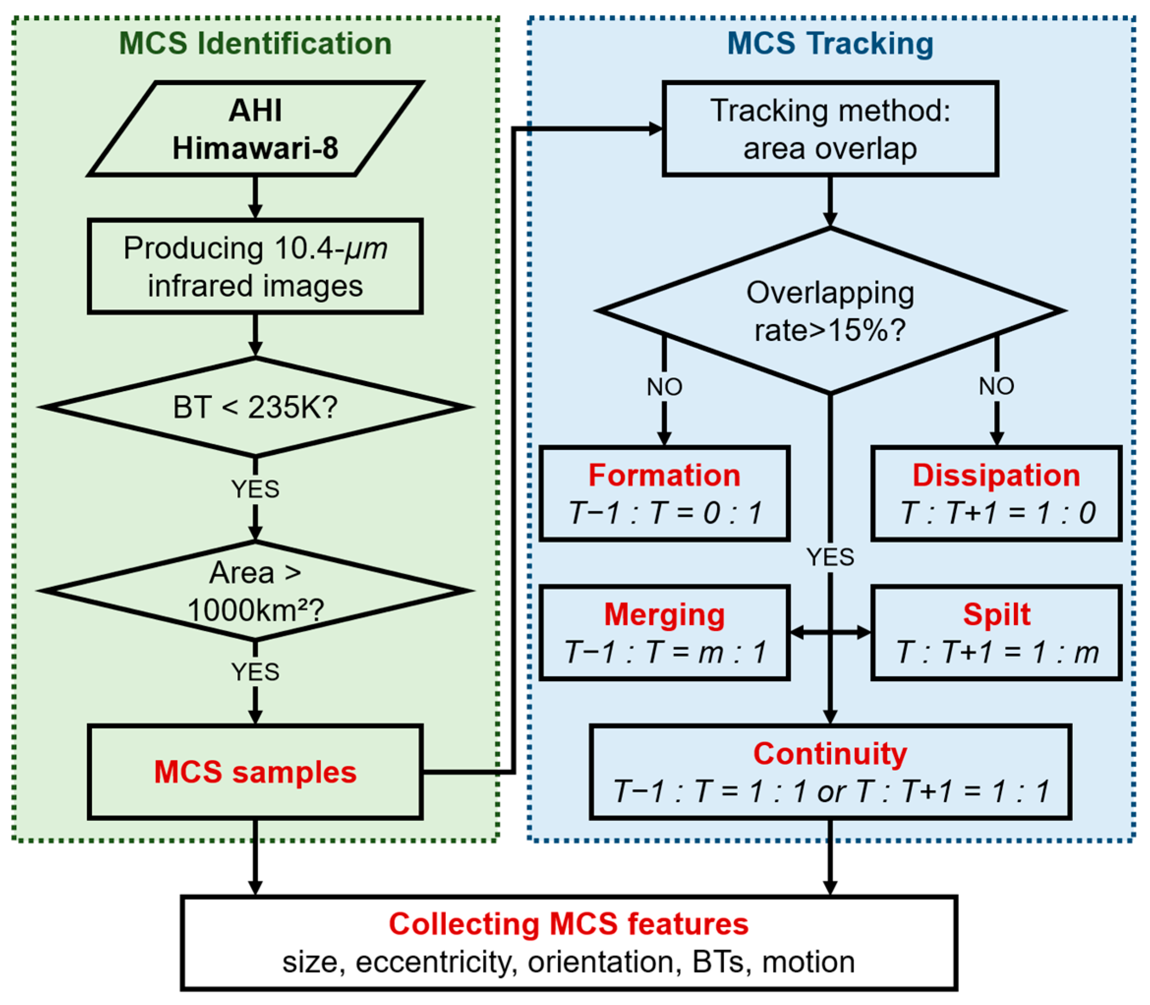
2.2. Identifying and Tracking MCSs

To date, geostationary satellite and ground-based radar observations are the two most useful materials to capture the life cycle of MCSs, due to their frequent sampling in both time and space. Nevertheless, geostationary satellite observations show some unique advantages over ground-based radar. First, it is easier to define and characterize MCSs by their contiguous cold cloud shields in satellite images than by their radar reflectivity patterns, where a board spectrum of underlying convection can occur [39]. That’s also why most of the automated methods to objectively identify and track MCSs rely on satellite images (e.g., [35,36,40,41]). Second, satellite observations allow for a broad spatial coverage in a unified viewpoint, which benefits the recognition of MCSs over complex underlying surfaces (e.g., southeastern China in this study) and the generalization of MCS results over different meteorological conditions [40]. By contrast, ground-based weather radars have relatively limited detection ranges, uneven sampling in the field of view, and often lack information over remote areas and complex terrains. Third, successive satellite images help to monitor the cloud evolution prior to the onset of significant radar-detected precipitation, which might aid in the nowcasting of MCSs [42].
There have been some studies investigating MCSs based on low-orbit satellite data (e.g., TRMM) [17,18] and satellite precipitation products (e.g., CMORPH) [22,42]. However, low-orbit satellite data have long revisit intervals and can only provide snapshots on the life cycle of MCSs. Though with a relatively short temporal interval (30–60 min), satellite precipitation products generally have a lower spatial resolution (~10 km) than geostationary satellite data. More importantly, satellite precipitation products have been proved to generally underestimate the precipitation in eastern and southern China during warm season [43,44], which could hamper the MCS investigation. For all the reasons above, we finally applied the geostationary satellite observations to investigate MCSs in this study. Specifically, the 10.4-μm infrared images available both day and night from Himawari-8 were utilized. This is a new-generation geostationary satellite that has a superior field of view over southeastern China and an unprecedented spatial resolution. How this Himawari-8 data were used to identify and track MCSs is briefly illustrated in Figure 2 and detailed as follows.
In a satellite infrared image at a certain time, an MCS sample is commonly identified as a contiguous cold cloud cluster with BTs lower than a given threshold and area larger than a given threshold (e.g., [15,35]). In this study, the BT and area thresholds were set as 235 K and 1000 km2, following some pioneering studies including one also based on Himawari-8 observations [35,40,45]. Such relatively moderate thresholds were chosen to capture the MCS lifecycle as completely as possible. Specifically, there were two major steps to define MCS samples in Himawari-8 infrared images (refer to the flowchart in Figure 2). The first step was to highlight cold cloud clusters with BTs lower than 235 K. The second step was to remove the small clusters with a size less than 1000 km2. The retained clusters were identified as MCS samples for the following analyses. Several typical examples of the identified MCS samples are given in Figure 3.
The identified MCS samples were tracked through the area overlap method, an automated method extensively used in previous studies (e.g., [40,45,46]). There is strong dependence of the overlapping rates on MCS size: Chen, et al. [35] showed most MCSs with a size of 1000–1500 km2 have an overlapping rate of more than 17.1% between 10-min satellite images; and Morel and Senesi [45] applied an overlapping rate of 15% to track MCSs with a pre-defined area of more than 1000 km2 in 30-min satellite images. As such, MCS samples in successive 10-min infrared images were considered to belong to the same MCS when their overlapping rate was higher than 15%.
By using the tracking method, five basic processes could be judged throughout the MCSs’ lifetimes (Figure 2), as in Vila, et al. [40]. A “formation” process was defined when an MCS sample had no MCS sample overlap in the previous satellite image, while a “dissipation” process was defined when an MCS sample had no MCS sample overlap in the next satellite image. If there was an overlap of only one pair of MCS samples in successive images, the MCS sample was deemed as undergoing a “continuity” process. When an MCS sample had more than one MCS sample overlap in the previous image, a “merging” process was declared, while a “spilt” process was declared when an MCS sample had more than one MCS sample overlap in the next image.

3. Overview of the Two Successive Warm-Sector Rainfall Episodes

On 6–7 May 2018, two rainfall episodes occurred in succession over southeastern China. Both episodes occurred in the warm sector to the south of a synoptic front propagating southeastward, as indicated by the high gradient belt of equivalent potential temperature (θe) in Figure 4a1–a4 (also refer to the front location analysis based on the surface weather maps in Figure S1 in the Supplementary Materials). Two rainfall episodes both began with the occurrence of local cloud clusters over southeastern China, which developed into MCSs in the following hours (Figure 5), ahead of a large-scale cloud shield associated with the synoptic front. The first rainfall episode (EP1 hereafter) started in the early morning on 6 May and dissipated at night. The second rainfall episode (EP2 hereafter) started at midnight on 7 May and its rainbands eventually merged with the frontal rainbands in the evening. Two 17-h periods were, respectively, selected for the following analyses of EP1 and EP2: 0500–2200 LST (LST = UTC + 8 h) on 6 May and 0000–1700 LST on 7 May.
Figure 6a,b show the distributions of rain-gauge-measured rainfall totals in EP1 and EP2, respectively. Notice that only the rainfalls at least 200 km away from the fronts were counted in order to ensure the rainfalls were warm-sector nature and less influenced by the fronts, as suggested in previous studies (e.g., [3,4,5]). Both EP1 and EP2 had a rainfall hotspot along the southeast coast of Fujian province, while EP2 had a cumulative rainfall maximum (290.5 mm) over four times that of EP1 (69.4 mm). In EP2, there was another >250 mm rainfall hotpot near eastern Guangdong province. Compared to EP1, EP2 had a stronger rain rate with remarkably more hourly rainfall of magnitude exceeding 20 mm (Figure 6c). Four hourly rainfalls of magnitude exceeding 100 mm were observed in EP2, with a maximum of 107.5 mm that was about twice that of the maximum in EP1 (51.6 mm). The maximum 1-h and 3-h rainfalls in EP2 were 1.2 and 2.4 times the local historical records, respectively [34]. This record-breaking rainfall event caused severe urban inundation and societal impacts in Xiamen (around 24.5°N, 118.0°E), a coastal city with a dense human population [33].
The two successive episodes occurred at the northwestern periphery of the western Pacific subtropical high, which gradually moved southeastward (indicated by the >5880 gpm region at 500 hPa in Figure 4a1–a4). During both episodes, there were similar mid-level southwesterlies with barely any shortwave perturbation; the southeastern coastal region was situated within the warm sector, more than 200 km ahead of the southeastward-moving front, and was controlled by warm and moist low-level southwesterly flows with 850-hPa θe higher than 340 K (Figure 4a1–a4). Notably, the 850-hPa θe over the southeastern coastal region increased by ~2–4 K from EP1 to EP2, which was likely due to the enhanced low-level southwesterly jet stream (>12 m s−1) over southeastern China in EP2.
Similar increments were observed in both precipitable water and convective available potential energy (CAPE) over southeastern China, especially along the coast, due to the intrusion of the moist and unstable airs from the South China Sea (Figure 4b1–b4). The vertical wind shear (VWS) of the 0–6 km AGL layer over southeastern China in EP2 (>16 m s−1 overall) was significantly larger than that in EP1 (<16 m s−1 overall), as revealed by the vectors in Figure 4b1–b4. Over the southeastern coast, there were stronger moisture flux convergence below the mid-troposphere in EP2 than in EP1, as indicated by more positive values in the vertically integrated moisture flux convergence [47] from 900 to 500 hPa (Figure S2 in the Supplementary Materials). Despite the relatively more favorable convective environment in EP2, operational numerical models (even those with a convection-permitting scale) show poor forecasting skill for this warm-sector torrential rainfall event [48]. This stimulates us to compare this disastrous warm-sector rainfall event with a normal warm-sector rainfall event from an observational perspective. Geostationary satellite observations often provide promising precursors in the nowcasting of convective storms (e.g., [49,50]), which could to some extent compensate for the deficiencies of numerical models.

4. Comparison of MCS Contributions and Features in the Two Rainfall Episodes

In this section, the roles and features of MCSs in EP1 and EP2 are compared. Since the MCSs were identified and tracked in 10-min satellite images, their linkages with rainfall were also considered within this 10-min framework. Whether an MCS sample contributed to rainfall is determined by the positional correspondence of the MCS sample identified in the 10-min satellite imagery and the 10-min rainfalls recorded by surface rain gauges. At a 10-min time stamp, when there were rain gauges occupied by an MCS sample, the rain-gauge-recorded rainfalls were attributed to the MCS sample and regarded as MCS-contributed rainfalls; otherwise, the rainfalls were regarded as non-MCS rainfalls.

4.1. MCS Contributions

In EP1 and EP2, MCSs accounted for 23.4% and 68.1% of the regional rainfall totals of 12,044 mm and 33,259 mm (via summing the rainfall totals measured by all rain gauges within southeastern China), respectively. It turns out that MCSs in EP1 contributed the vast majority of the rainfall amounts at many inland sites but contributed less (mostly <30%) along the coast, including the rainfall hotspot of EP1 (Figure 7a). By contrast, prominent MCS contributions (>60%) in EP2 were observed at both inland and coastal sites (Figure 7b). For the two coastal rainfall hotspots in EP2 (Figure 6b), the MCS contributions generally exceeded 80%.
The MCS contribution as a function of cumulative rainfall was further investigated by dividing the rainfall samples within southeastern China into six subsets according to rainfall magnitude. In EP1, all of the subsets had over half of the samples with an MCS contribution less than 10% (Figure 7c). Overall, the MCS contribution was most significant for the 10–20 mm subset, in which about 30% of the samples had an MCS contribution larger than 50%. The MCS contributions were totally less than 30% for the ≥50 mm subset in EP1, which was probably because the heavy rainfall in EP1 was mainly induced by convective storms smaller than the MCS scale and shallow convection with low cloud top (BT ≥ 235 K). Compared to EP1, the MCS contribution in EP2 was much larger and increased as the cumulative rainfall increased (Figure 7d). For the ≥50 mm subset in EP2, over 80% of the samples had an MCS contribution of more than 50%, and over half of the samples had an MCS contribution of more than 90%. These results suggest a more dominant role played by MCSs in producing the rainfall totals, especially the heavy rainfall totals, in EP2.
Moreover, MCSs played a more important role in generating more intense rainfall within a short duration in both episodes. This is evidenced by the increasing trend in the proportion of MCS-related samples as the 10-min rainfall increased from 0–5 mm to ≥20 mm (Figure 7e,f). However, the MCS contributions to different ranges of 10-min rainfall in EP1 were not so significant as in EP2. In a lower range of the 10-min rainfall in EP1, a higher proportion of samples could be attributed to non-MCS systems, again, consisting of the small isolated convective storms and shallow convection. For the subset with 10-min rainfall over 20 mm, all of the samples in EP2 were contributed by MCSs, whereas only half of the samples in EP1 were contributed by MCSs.
In summary, MCSs demonstrated a more significant rainfall contribution in EP2 than in EP1, in terms of both rainfall intensity and total. It is speculated that the MCS features might have differed between the two episodes and thus affected the MCS-related rainfalls, which is examined in the next subsection.

4.2. General Features of MCSs

During EP1 and EP2, there were 8 and 21 MCSs developing over southeastern China, with 113 and 224 MCS samples identified throughout their life cycle based on the Himawari-8 infrared images at 10-min interval, respectively. The MCS activities created a wider MCS pathway in EP2 than in EP1, also with higher MCS frequency along the pathway (Figure 8a,b). In EP2, there were over 15,000 satellite pixels (nearly 60,000 km2) that had an MCS frequency larger than 15%; while in EP1, the MCS frequencies were all below 15%. In each episode, the high-MCS-frequency center was observed nearby the coastal rainfall hotspot (Figure 6a,b). In EP2, the two rainfall hotspots had an MCS occurrence frequency up to 40% or higher. These results indicate that the production of warm-sector heavy rainfall was associated with the repeated passage of MCS samples.
The MCS tracks showed that the earlier MCS samples in EP1 and EP2 both originated from eastern Guangdong and propagated eastward (Figure 8a,b). The MCSs in EP1 consistently remained separate, without any merging processes, during their life cycle (Figure 5a1–a4 and Figure 8a). By contrast, most of the MCSs in EP2 underwent at least one merging process (Figure 5b1–b4 and Figure 8b). This resulted in the most long-lived MCS of up to 10 h, which was the primary producer of the warm-sector rainfall hotspot over coastal Fujian.
Overall, the MCS samples in EP2 were significantly larger than those in EP1 (Figure 9a). On average, the MCS sizes in EP1 and EP2 were 954 and 2469 satellite pixels, respectively. About 51.8% of the MCS samples in EP2 were larger than 1000 pixels, while this was only 33.6% in EP1. The maximum size was 13,244 pixels and belonged to the most long-lived MCS in EP2. The frequent merging between MCSs in EP2 could have facilitated the maintenance and areal expansion of MCSs [20,41]. The greater 0–6 km VWS in EP2 mentioned previously (Figure 4b1–b4) could have helped organize local storms into larger MCSs [16] and generate stronger precipitation [39], especially over the coastal region where precipitable water was abundant (Figure 4b1–b4).
Most MCS samples in both episodes had a linear (or elongated) shape in the satellite images, with an eccentricity (i.e., minor axis/major axis) [41] less than 0.5 (Figure 9b). Only a few MCS samples in EP2 satisfied the common satellite-based definition (i.e., eccentricity > 0.7) of a circular MCS (e.g., [36,39]). Despite the similar linear MCS shape in both episodes, the MCS orientation differed greatly between the episodes (Figure 9c). In EP1, the majority of MCS samples were orientated southeast–northwest (~50%) and north–south (~37%). By contrast, in EP2, an east–west orientation was most common (~58%), followed by northeast–southwest (~27%). The strong eastward/northeastward VWSs (Figure 4b1–b4) in EP2 may have led to MCSs developing on the down-shear side and orienting along the shear direction [16], mainly via an organization mode of back-building [48].
The investigation of MCS motion was only based on the MCS samples without a merging or splitting process, in order to avoid the unreliable motion caused by the sudden displacement of an MCS sample. An overall faster MCS movement was seen in EP1, with an average (median) speed of 18.4 (17.5) m s−1, versus 15.3 (15.3) m s−1 in EP2 (Figure 9d). A slower-moving MCS should be more efficient in producing local torrential rainfall totals, and this is particularly true when a linear MCS moves along its orientation to generate the “training” effect—a repeated passage of convective elements within the MCS over a given area (e.g., [16,23,26]). Within the prevailing westerly and southwesterly flows (Figure 4a1–a4), over 90% of the MCS samples in each episode moved eastward or northeastward (Figure 9e). Such directions were more parallel to the dominant east–west and northeast–southwest orientations of the MCSs in EP2, while they were more perpendicular to the dominant southeast–northwest and north–south orientations in EP1. Consequently, the consistency between the MCS orientation and moving direction in EP2 demonstrated the considerable potential of the “training” process, as confirmed by the radar analyses in Hu, et al. [33].
The MCS intensity was considered via two BT-based approaches: the BT averages of all MCS pixels (Figure 9f) and the 25% coldest MCS pixels (Figure 9g). Either approach showed an overall stronger intensity (i.e., colder BT) of the MCS samples in EP2 than in EP1, albeit with a more apparent distinction in the latter, with the median being 219 K in EP1 versus 216 K in EP2. The MCS hotspots in EP2 (MCS frequency > 30%) possessed overall lower BTs and thus more intense MCS activities than their EP1 counterparts (MCS frequency > 10%) (Figure 8c,d). For the common hotspot around 118°E, the EP2 BTs were down to 210 K, almost 10 K lower than their EP1 counterparts. There were also some other fairly low BT areas in both EP1 (around 116.3°E, 23.8°N) and EP2 (around 116°E, 23.8°N). However, the MCS samples were not frequent (<10%) therein, and accordingly did not produce warm-sector heavy rainfall as the MCS hotspots in EP2 did (Figure 6a,b). Compared to EP1, the greater VWSs in EP2 could promote upscale growth of convection (a result of the interaction between VWSs and cold pool of convection) and thus the formation of more organized MCSs [16,51]. These MCSs appeared to have stronger convective intensity and thus higher cloud tops (i.e., lower BTs), largely due to the higher CAPE environment in EP2.

4.3. Rainfall Potential Indices Derived from MCS Features

The results above highlight two key processes associated with MCSs in warm-sector rainfall production: the repeated passage (or long passing time) of an individual MCS over given areas (i.e., the “training” effect) and the merging processes between MCSs. Nonetheless, proper criteria to objectively diagnose them are still lacking. To this end, two indices involving MCS features are proposed here, called the overlap index (OLI) and merging potential index (MPI).
OLI estimates the integrated probability of overlap (i.e., repetition) of MCS area along the pathway of an individual MCS in the following hour, by assuming constant MCS features. Specifically, OLI is computed for each identified MCS sample of “continuity” status since it has reliable movement information. The calculation is performed within the framework of the spatial (2 km) and temporal (10 min) resolutions of Himawari-8 infrared images and consists of the following three procedures (Figure 10). First, the MCS sample is extrapolated for one hour (i.e., six more 10-min timestamps) according to the MCS motion. Second, for each MCS pixel over the extrapolating pathway, overlap ratio is calculated as the overlap number divided by seven, that is, the total timestamp number for one hour. If the overlap number is seven, it means the pixel is occupied by the MCS for the full one hour. Third, the overlap ratios throughout the MCS pixels over the extrapolating pathway are averaged to obtain an integrated percentage of overlap, that is, OLI.
A larger, slower-moving linear MCS sample produces a higher OLI, especially when it moves more along its orientation (Figure 10). Based on all the MCS samples of “continuity” status, it appears that the OLI magnitudes in EP1 were significantly lower than in EP2, with respective medians of 42% and 57% (Figure 11a). The higher OLI indicated a greater potential of longer passing time of an individual MCS (i.e., repeated passing of the MCS samples) over given areas, such as the MCS hotspots in EP2 (Figure 8b).
MPI quantifies the potential for merging processes in each MCS sample, by summing its fractional distance or distances with the other MCS sample or samples within its 400 km range (Figure 12). An MCS sample has a higher MPI when it is surrounded by more and closer MCS samples, and thus has a higher potential for merging occurrence. In the current study, MPI was significantly lower in EP1 than in EP2, with respective averages of 1.0 and 2.1 (Figure 11b). This result was consistent with the track-based results in which merging was frequently observed in EP2 but not in EP1 (Figure 5 and Figure 8a,b).
It seems that OLI and MPI can serve as practical indicators for subsequent rainfall production. All the MCS samples in the two episodes were divided into four subsets according to their OLI/MPI magnitudes (Figure 13a,b). Generally, the MCSs with a higher OLI/MPI were more capable of producing stronger maximum rainfall in the next hour (calculated as the average of the top five hourly rainfalls belonging to an MCS sample, to avoid overestimation by a single extreme rainfall sample). For instance, ~80% of MCS samples with <40% OLI produced only light (<5 mm) hourly maximum rainfall, while ~70% of MCS samples with ≥60% OLI produced hourly maximum rainfall over 20 mm. This is also demonstrated by the two specific samples shown in Figure 13c,d. These two MCS samples both appeared nearby the coast and had a similar size of between 1000 and 1200 pixels, but the one with higher OLI and MPI produced a maximum rainfall of 43.5 mm in the following hour, which was about 2.5 times that of the other one (17.7 mm). Similar results were obtained when investigating the maximum 10-min rainfall over the next hour (Figure 14). The potential of OLI and MPI as precursors shows great promise in aiding the nowcasting of rainfall produced by MCSs.

5. Discussion

In this study, observations from the geostationary satellite Himawari-8 were utilized to investigate MCSs from a perspective of cloud cluster. It has to be admitted that although geostationary satellite images provide an effective way of identifying MCSs, they lack detail information on the structure of the underlying convection and internal precipitation [39,52]. Observations from ground-based weather radars may be helpful in addressing this issue, which requires further investigation.
Two newly proposed indices were proved to be indicative for heavy rainfall production based on the MCS samples in the two rainfall episodes examined in this work. To further confirm their applicability with more cases, we additionally collected 319 MCS samples that occurred over southern China on another two days (3–4) in May 2018 and examined the two indices. Similarly, as in EP1 and EP2, these newly collected MCS samples tended to produce larger maximum rainfall amount and stronger maximum 10-min rainfall in the next hour when their OLI and MPI were higher (Figure S3 in the Supplementary Materials). Nevertheless, statistical studies over a larger MCS database to demonstrate the applicability of the two indices in different scenarios and explore critical values for rainfall nowcasting are still needed and will be conducted in the near future.

6. Conclusions

As a typical rainfall type over South China, warm-sector rainfall is often attributed to MCSs. However, the MCS contribution to warm-sector rainfall is rarely well-quantified, and the potential distinction of MCS behaviors in different warm-sector rainfall events remains unexplored. On 6–7 May 2018, two warm-sector rainfall episodes (EP1 and EP2) occurred in succession over southeastern China, with EP2 breaking historical rainfall records and producing a maximum rainfall total over four times that of EP1. The purpose of the present study was to elucidate how MCSs behaved in these two back-to-back but distinct warm-sector episodes, and thus explore the distinct role of MCSs in warm-sector rainfall. MCSs were identified, tracked, and characterized based on Himawari-8 infrared images. The main findings can be concluded as follows:
(1)
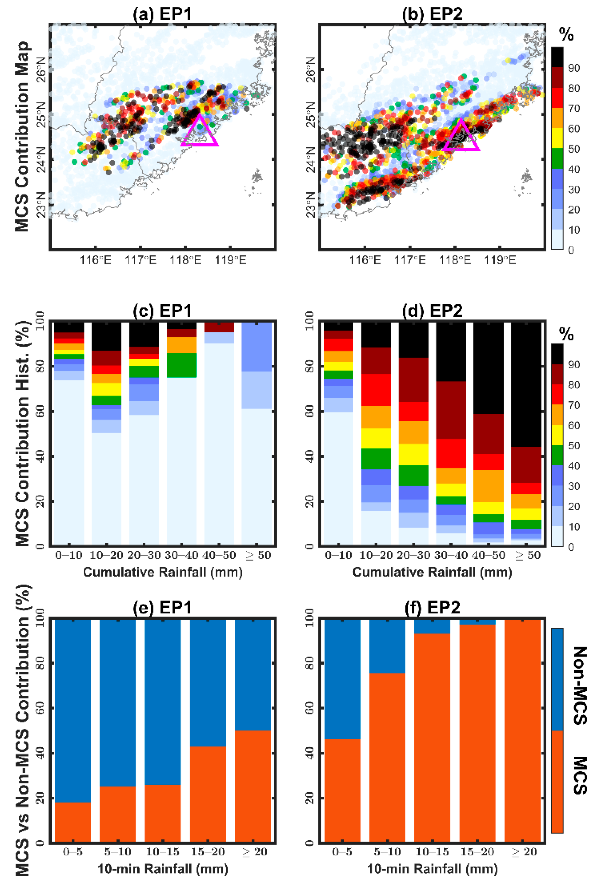
MCSs dominated the rainfall production in EP2 but not in EP1. For the regional warm-sector rainfall total, the MCS contribution was 23.4% in EP1 versus 68.1% in EP2. An overall increasing MCS contribution was observed in the larger cumulative rainfall ranges in EP2; particularly, MCSs accounted for over 80% of the coastal extreme warm-sector rainfall total. By contrast, the MCSs in EP1 contributed more to the rainfall totals between 10–30 mm. Both episodes showed an increasing MCS proportion in the stronger 10-min rainfall intensity, but the proportions in EP2 were 2–4 times their EP1 counterparts.
(2)
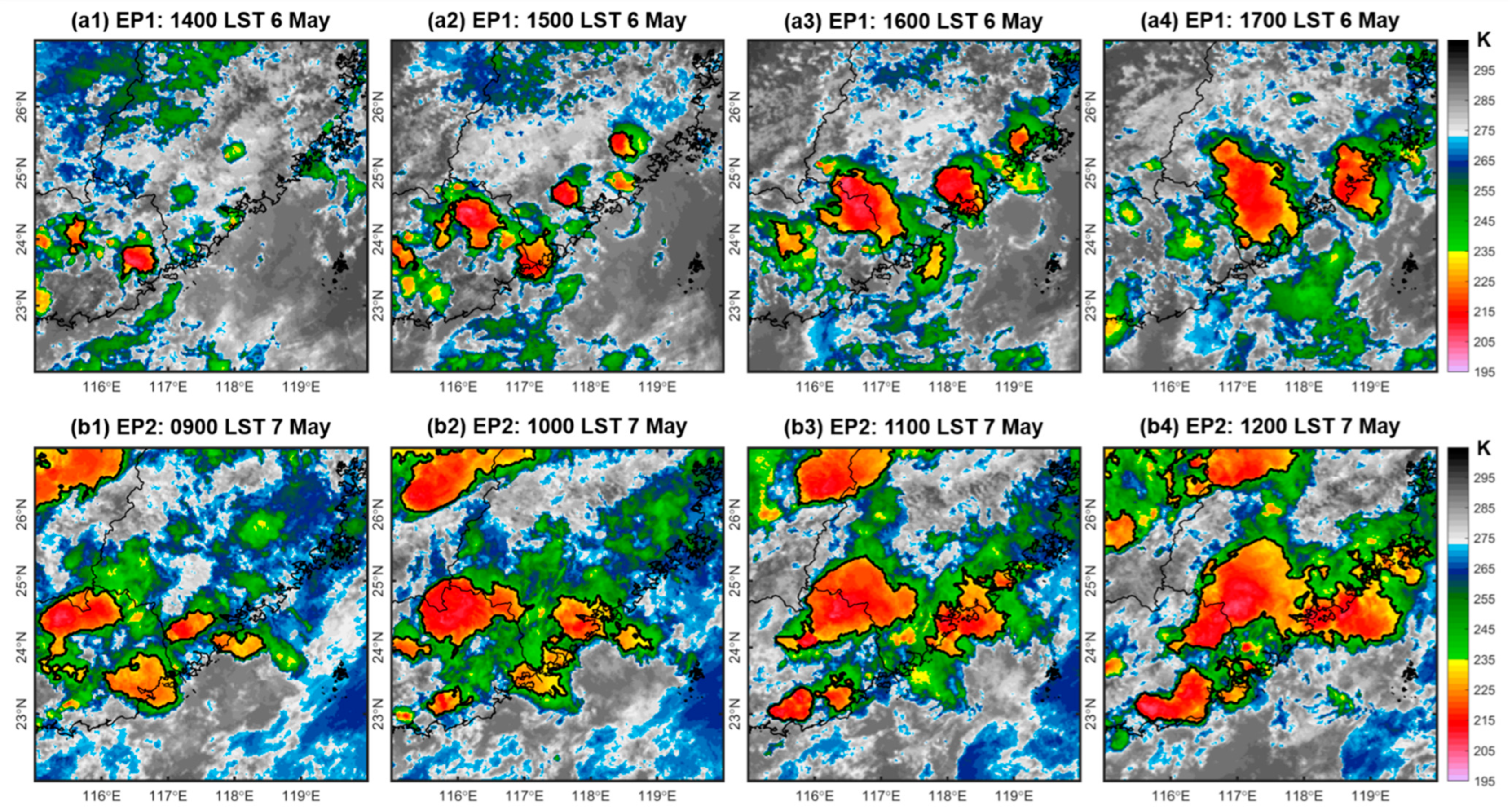
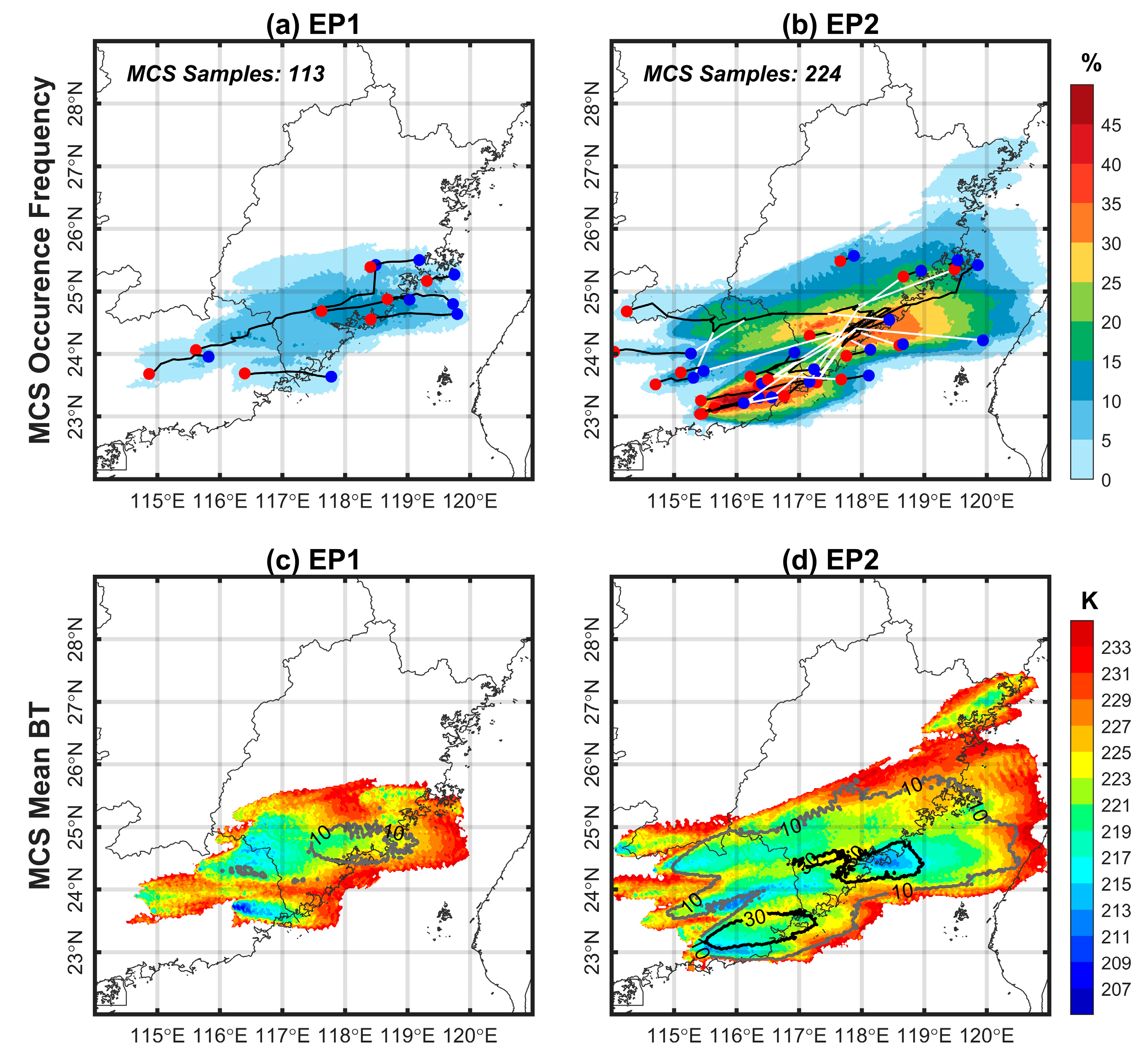
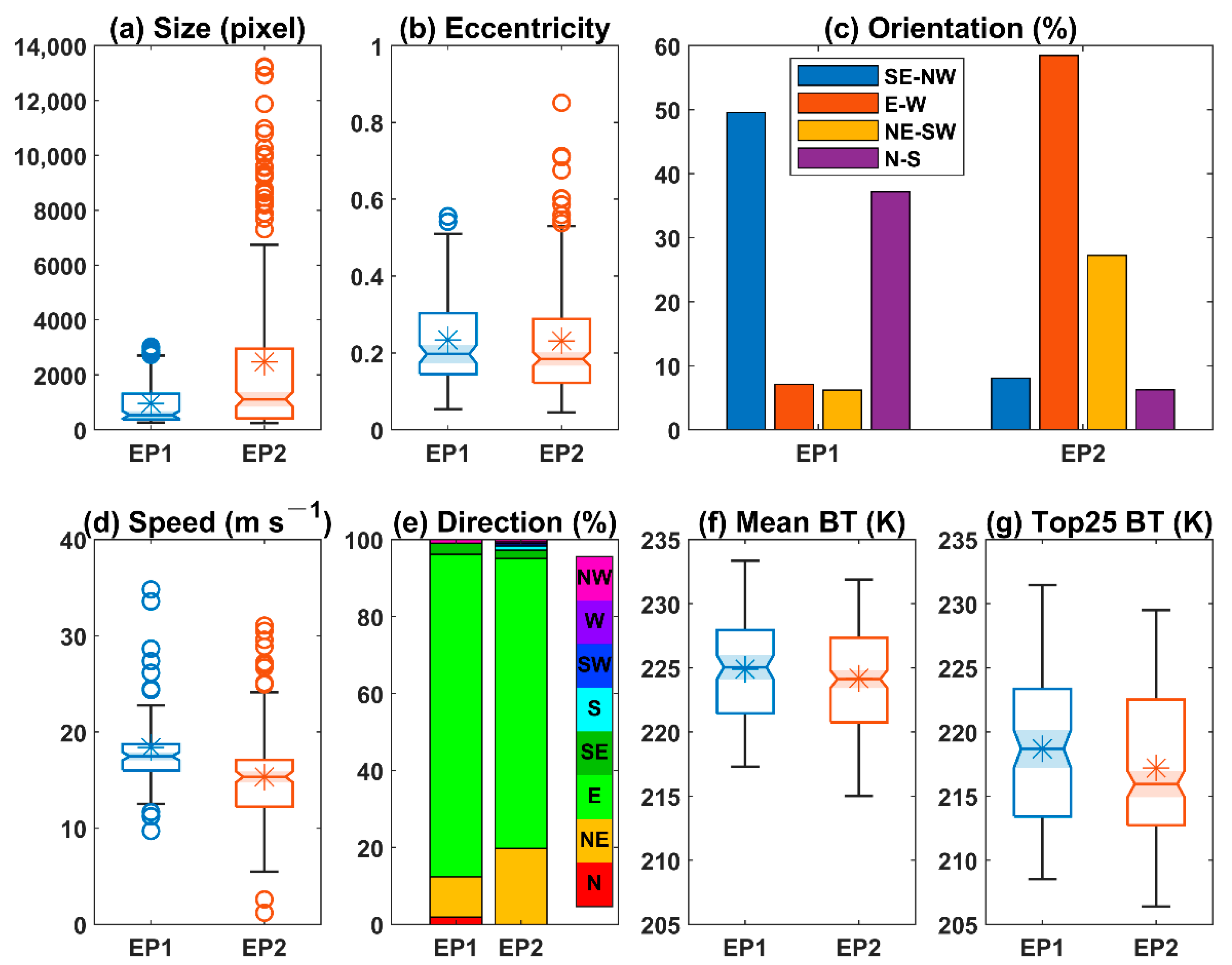
MCS occurrence was more frequent in EP2 than in EP1, especially in the coastal rainfall hotspots where MCSs appeared for over six hours. Merging between MCSs occurred frequently in EP2 and resulted in long-lived and extensive MCSs, but this process was absent in EP1. Overall, the MCS samples in EP2 were much larger in size, more intense, and moved slower than their EP1 counterparts, which were favorable for rainfall production in EP2. Despite having dominant eastward and northeastward motions in both episodes, MCSs tended to move parallel to their orientation in EP2 (east–west and northeast–southwest), while perpendicular in EP1 (southeast–northwest and north–south). The parallelism in EP2 between the MCS moving direction and orientation was able to generate a “training” effect (i.e., long passing time of an individual MCS over given areas) and thus promote local rainfall accumulation.
(3)
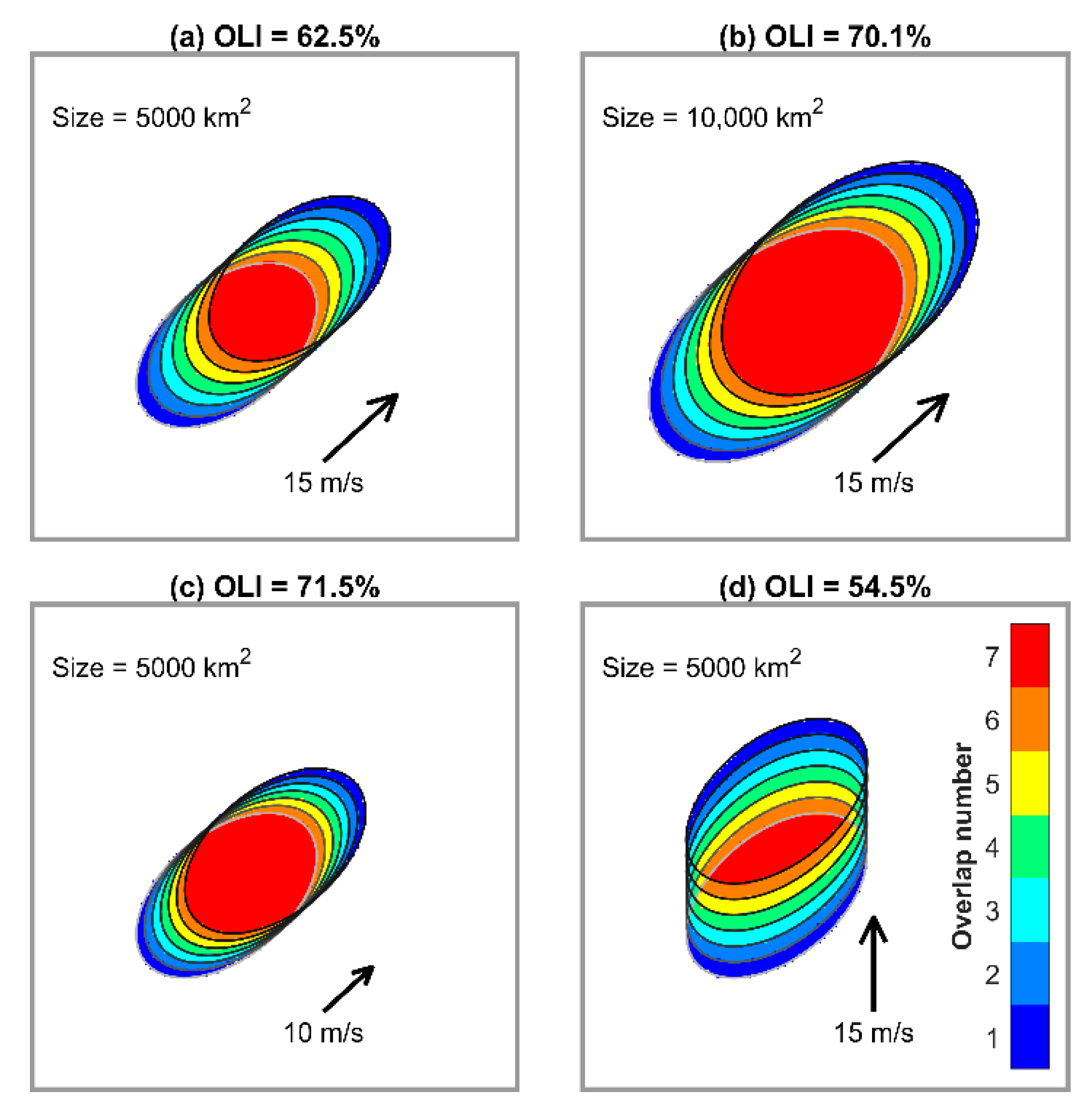
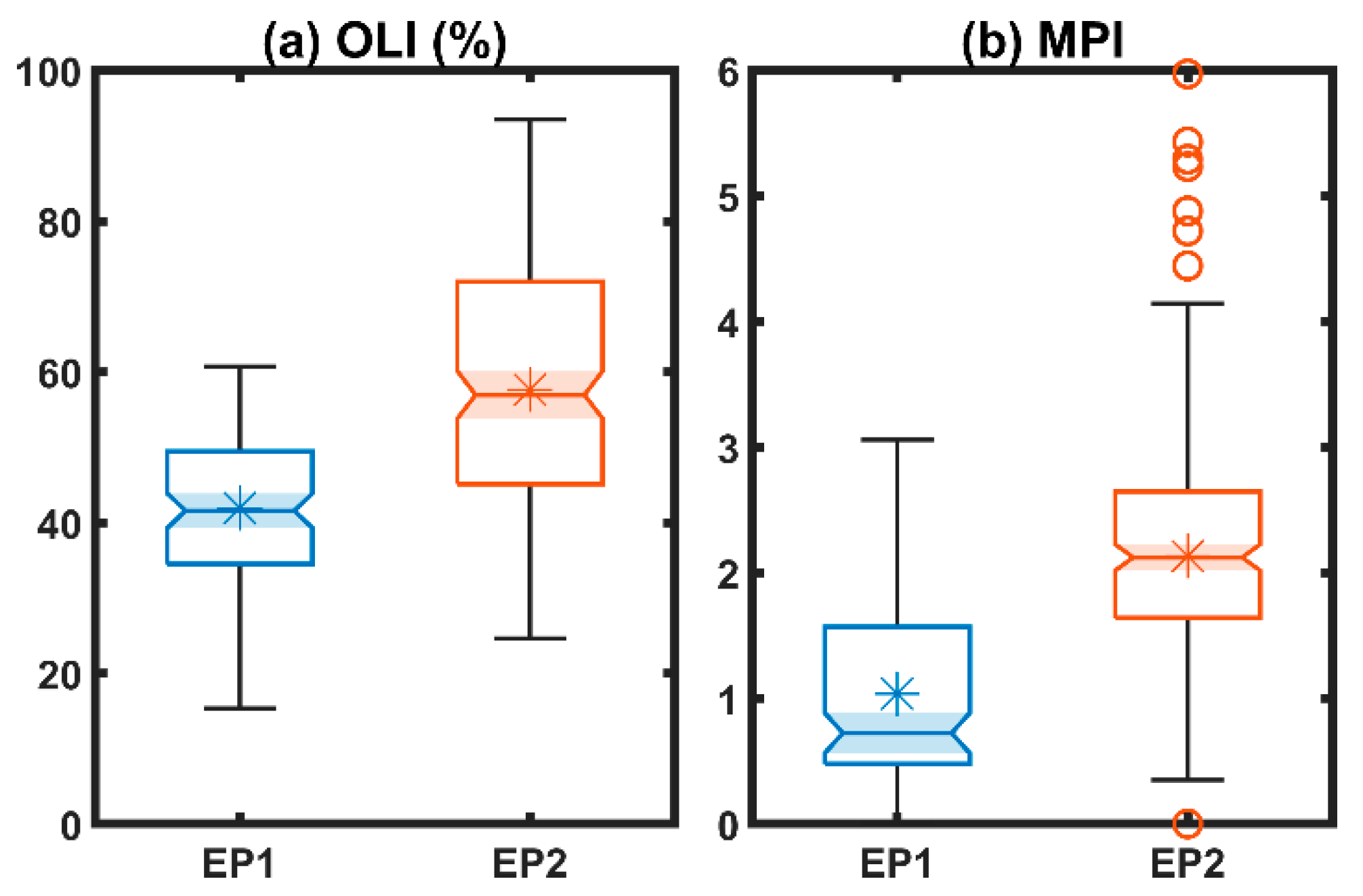
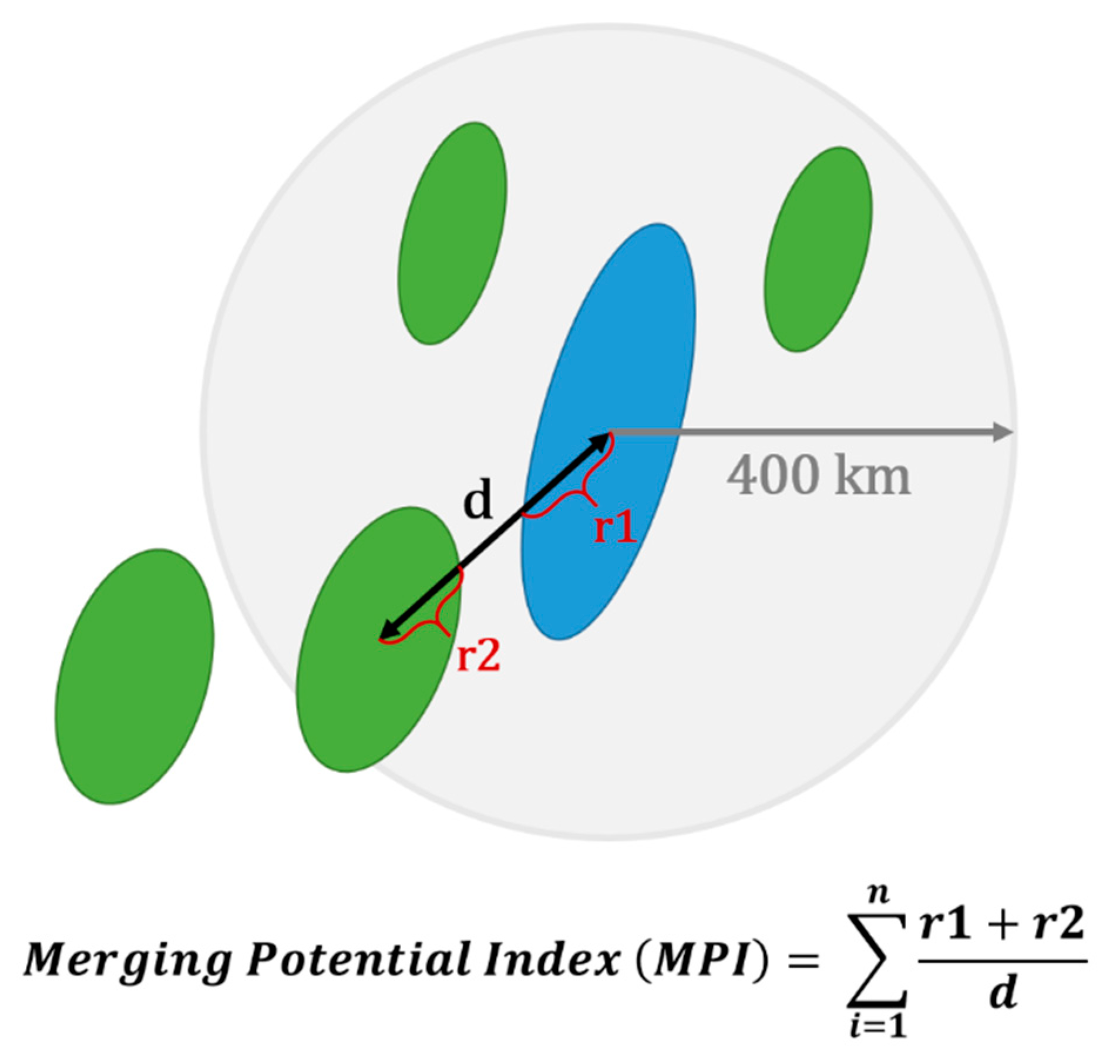
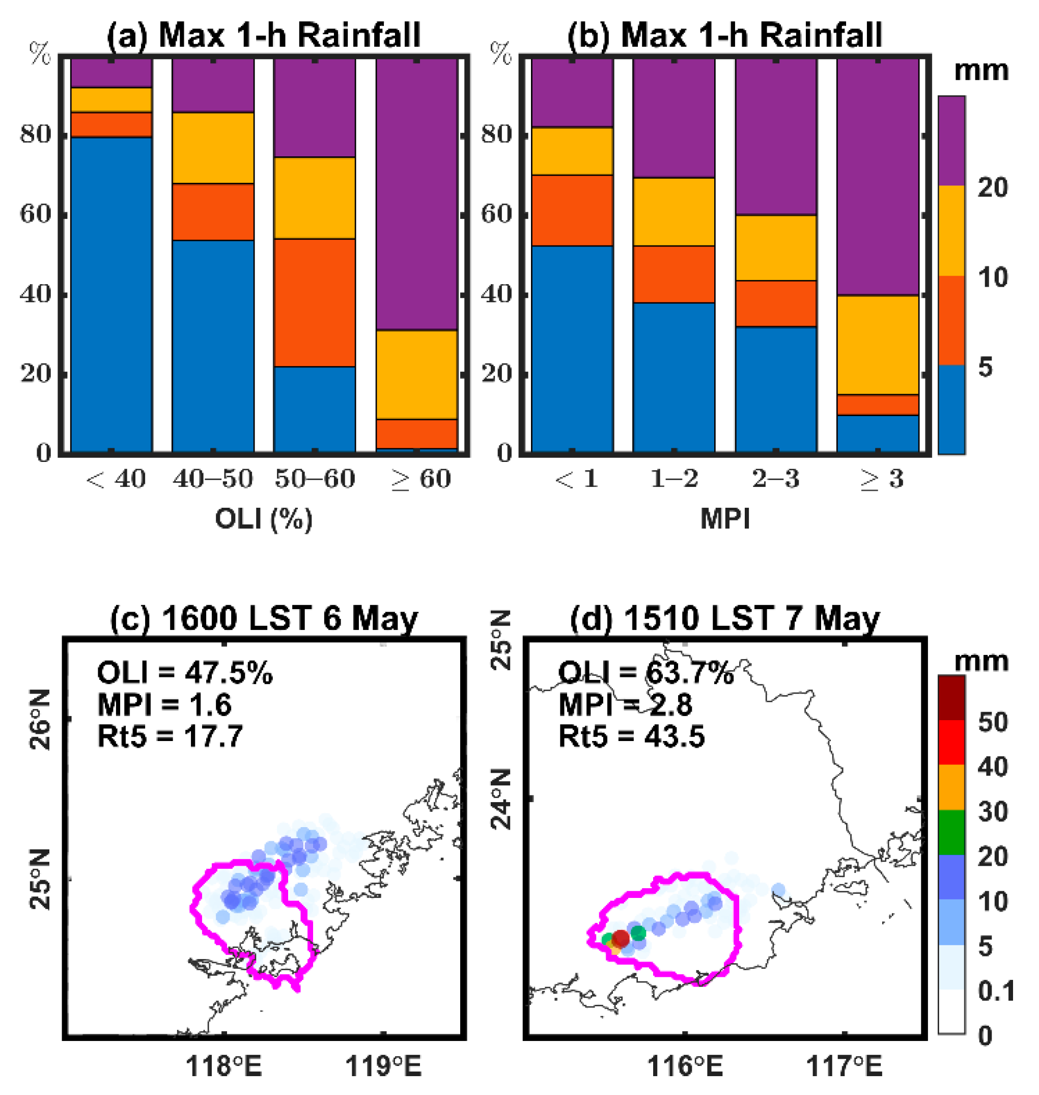
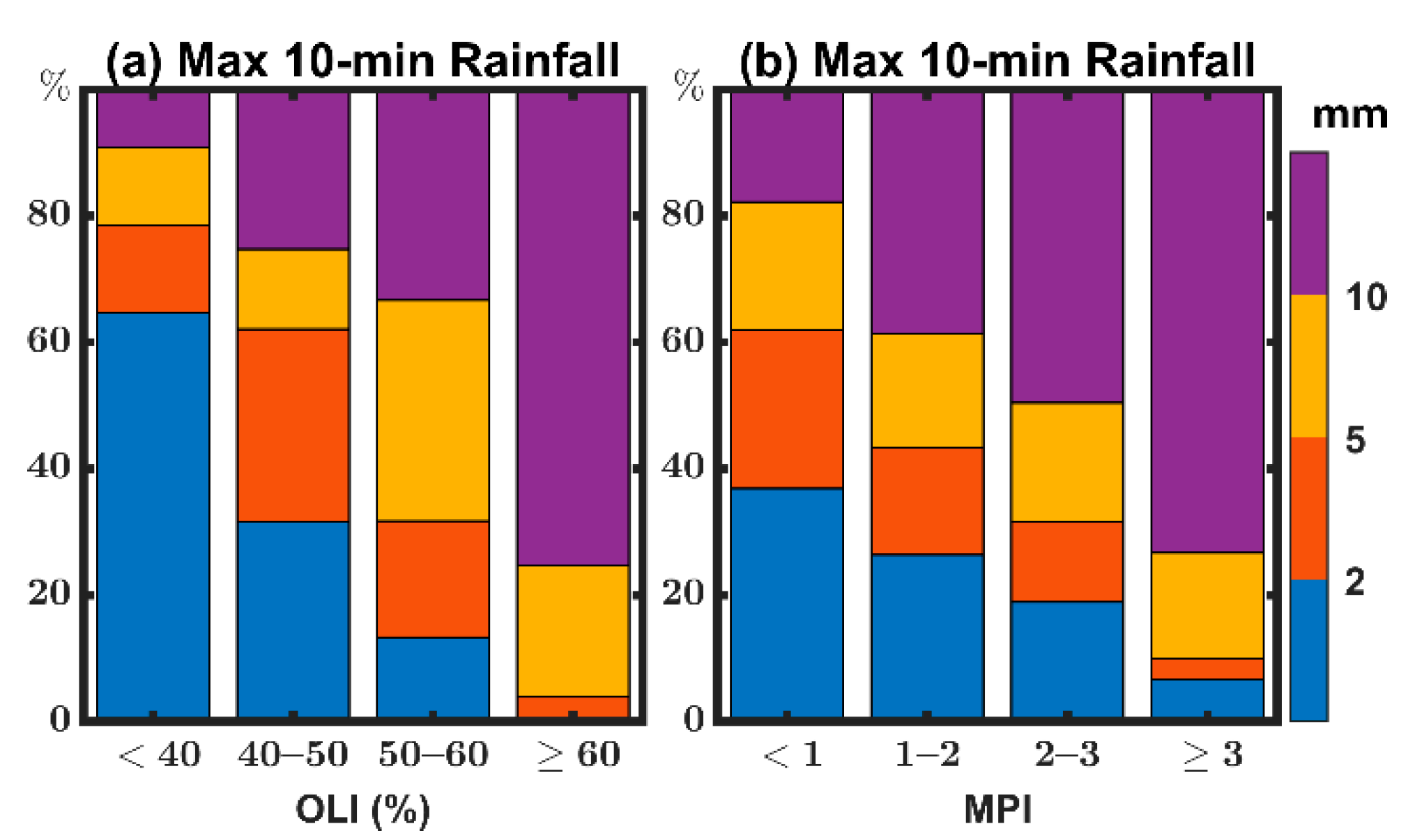
Based on MCS features, two practical indices––OLI and MPI––were proposed to evaluate two MCS processes vital for rainfall production: the repeated passage of an individual MCS over given areas and the merging processes between MCSs, respectively. The significantly higher OLI and MPI in EP2 than in EP1 demonstrated the greater potential of these two effects. A larger OLI/MPI magnitude generally indicated a larger maximum rainfall amount in the following hour, along with a stronger maximum 10-min rainfall. Nearly 70% (60%) of MCS samples with OLI (MPI) exceeding 60% (3) produced heavy rainfall of over 20 mm in the next hour.
This paper demonstrates the distinct role of MCSs in two successive warm-sector rainfall episodes and relates the distinction to the differences in satellite-observed MCS features. The proposed indices involving MCS features show considerable promise in offering information in advance of rainfall production. It is thus envisioned that a real-time MCS analysis based on geostationary satellite images at frequent temporal intervals would facilitate rainfall nowcasting, which is particularly meaningful for the warm-sector rainfall with limited predictability in numerical models.

Supplementary Materials

The following supporting information can be downloaded at: https://www.mdpi.com/article/10.3390/rs14215434/s1, Figure S1: surface weather maps at 6-h interval between 0800 LST on 6 May 2018 and 1400 LST on 7 May 2018; Figure S2: distribution of vertically integrated moisture flux convergence from 900 to 500 hPa and moisture flux at 850 hPa for the two warm-sector rainfall episodes; Figure S3: distributions of the maximum rainfall amount and 10-min rainfall in the next hour produced by the 319 MCS samples over southern China on 3–4 May 2018, as a function of OLI and MPI.

Author Contributions

Conceptualization, Y.H. and M.Z.; methodology, Y.H. and M.Z.; software, Y.H.; validation, Y.H. and M.Z.; formal analysis, Y.H. and M.Z.; investigation, Y.H.; resources, Y.H. and M.Z.; data curation, Y.H.; writing—original draft preparation, Y.H. and M.Z.; writing—review and editing, Y.H. and M.Z.; visualization, Y.H.; supervision, M.Z.; project administration, Y.H. and M.Z.; funding acquisition, Y.H. and M.Z. All authors have read and agreed to the published version of the manuscript.

Funding

This research was funded by the National Natural Science Foundation of China, grant number 41905049, the China Postdoctoral Science Foundation, grant number 2021M702725, and the Xiamen Science and Technology Program, grant number 3502Z20206079. M.Z. is also sponsored by the MEL Outstanding Postdoctoral Scholarship from Xiamen University.

Data Availability Statement

Not applicable.

Acknowledgments

The Himawari-8 data were downloaded from the P-Tree system of the Japan Aerospace Exploration Agency (JAXA) at https://www.eorc.jaxa.jp/ptree/index.html (accessed on 8 August 2021). The ERA5 reanalysis data were provided by ECMWF and downloaded from Copernicus Climate Change Service Climate Data Store at https://cds.climate.copernicus.eu (accessed on 10 June 2021). The rain gauge data and surface weather maps were provided by the China Meteorological Administration, and the radar mosaics of southeastern China were provided by the Fujian Meteorological Bureau. We thank the Editor and three anonymous reviewers for their constructive comments.

Conflicts of Interest

The authors declare no conflict of interest.

References

  1. Luo, Y.; Zhang, R.; Wan, Q.; Wang, B.; Wong, W.K.; Hu, Z.; Jou, B.J.-D.; Lin, Y.; Johnson, R.H.; Chang, C.-P.; et al. The Southern China Monsoon Rainfall Experiment (SCMREX). Bull. Am. Meteorol. Soc. 2017, 98, 999–1013. [Google Scholar] [CrossRef]
  2. Huang, S.; Li, Z.; Bao, C.; Yu, Z.; Chen, H.; Yu, S.; Li, J.; Peng, B.; Sun, S.; Zhu, Q.; et al. Heavy Rainfall over Southern China in the Pre-Summer Rainy Season; Guangdong Science and Technology Press: Guangdong, China, 1986; p. 244. [Google Scholar]
  3. Wu, N.; Ding, X.; Wen, Z.; Chen, G.; Meng, Z.; Lin, L.; Min, J. Contrasting frontal and warm-sector heavy rainfalls over South China during the early-summer rainy season. Atmos. Res. 2020, 235, 104693. [Google Scholar] [CrossRef]
  4. Li, X.; Du, Y. Statistical Relationships between Two Types of Heavy Rainfall and Low-Level Jets in South China. J. Clim. 2021, 34, 8549–8566. [Google Scholar] [CrossRef]
  5. Zhang, M.; Meng, Z. Warm-Sector Heavy Rainfall in Southern China and its WRF Simulation Evaluation: A Low-Level-Jet Perspective. Mon. Weather Rev. 2019, 147, 4461–4480. [Google Scholar] [CrossRef]
  6. Du, Y.; Chen, G. Climatology of Low-Level Jets and Their Impact on Rainfall over Southern China during the Early-Summer Rainy Season. J. Clim. 2019, 32, 8813–8833. [Google Scholar] [CrossRef]
  7. Zhang, M.; Rasmussen, K.L.; Meng, Z.; Huang, Y. Impacts of Coastal Terrain on Warm-Sector Heavy-Rain-Producing MCSs in Southern China. Mon. Weather Rev. 2022, 150, 603–624. [Google Scholar] [CrossRef]
  8. Du, Y.; Chen, G.; Han, B.; Bai, L.; Li, M. Convection Initiation and Growth at the Coast of South China. Part II: Effects of the Terrain, Coastline, and Cold Pools. Mon. Weather Rev. 2020, 148, 3871–3892. [Google Scholar] [CrossRef]
  9. Chen, X.; Zhang, F.; Zhao, K. Diurnal Variations of the Land–Sea Breeze and Its Related Precipitation over South China. J. Atmos. Sci. 2016, 73, 4793–4815. [Google Scholar] [CrossRef]
  10. Wu, M.; Luo, Y. Mesoscale observational analysis of lifting mechanism of a warm-sector convective system producing the maximal daily precipitation in China mainland during pre-summer rainy season of 2015. J. Meteorol. Res. 2016, 30, 719–736. [Google Scholar] [CrossRef]
  11. Yin, J.; Zhang, D.-L.; Luo, Y.; Ma, R. On the Extreme Rainfall Event of 7 May 2017 over the Coastal City of Guangzhou. Part I: Impacts of Urbanization and Orography. Mon. Weather Rev. 2020, 148, 955–979. [Google Scholar] [CrossRef]
  12. Wu, M.; Luo, Y.; Chen, F.; Wong, W.K. Observed Link of Extreme Hourly Precipitation Changes to Urbanization over Coastal South China. J. Appl. Meteorol. Climatol. 2019, 58, 1799–1819. [Google Scholar] [CrossRef]
  13. Huang, L.; Luo, Y. Evaluation of quantitative precipitation forecasts by TIGGE ensembles for south China during the presummer rainy season. J. Geophys. Res. Atmos. 2017, 122, 8494–8516. [Google Scholar] [CrossRef]
  14. Du, Y.; Chen, G. Heavy Rainfall Associated with Double Low-Level Jets over Southern China. Part I: Ensemble-Based Analysis. Mon. Weather Rev. 2018, 146, 3827–3844. [Google Scholar] [CrossRef]
  15. Houze, R.A. 100 Years of Research on Mesoscale Convective Systems. Meteorol. Monogr. 2018, 59, 1–54. [Google Scholar] [CrossRef]
  16. Schumacher, R.S.; Rasmussen, K.L. The formation, character and changing nature of mesoscale convective systems. Nat. Rev. Earth Environ. 2020, 1, 300–314. [Google Scholar] [CrossRef]
  17. Nesbitt, S.W.; Cifelli, R.; Rutledge, S.A. Storm Morphology and Rainfall Characteristics of TRMM Precipitation Features. Mon. Weather Rev. 2006, 134, 2702–2721. [Google Scholar] [CrossRef] [Green Version]
  18. Liu, C. Rainfall Contributions from Precipitation Systems with Different Sizes, Convective Intensities, and Durations over the Tropics and Subtropics. J. Hydrometeorol. 2011, 12, 394–412. [Google Scholar] [CrossRef] [Green Version]
  19. Roca, R.; Fiolleau, T. Extreme precipitation in the tropics is closely associated with long-lived convective systems. Commun. Earth Environ. 2020, 1, 18. [Google Scholar] [CrossRef]
  20. Zhang, L.; Min, J.; Zhuang, X.; Schumacher, R.S. General Features of Extreme Rainfall Events Produced by MCSs over East China during 2016–17. Mon. Weather Rev. 2019, 147, 2693–2714. [Google Scholar] [CrossRef]
  21. Haberlie, A.M.; Ashley, W.S. A Radar-Based Climatology of Mesoscale Convective Systems in the United States. J. Clim. 2019, 32, 1591–1606. [Google Scholar] [CrossRef]
  22. Li, P.; Moseley, C.; Prein, A.F.; Chen, H.; Li, J.; Furtado, K.; Zhou, T. Mesoscale Convective System Precipitation Characteristics over East Asia. Part I: Regional Differences and Seasonal Variations. J. Clim. 2020, 33, 9271–9286. [Google Scholar] [CrossRef]
  23. Luo, Y.; Xia, R.; Chan, J.C.L. Characteristics, Physical Mechanisms, and Prediction of Pre-summer Rainfall over South China: Research Progress during 2008–2019. J. Meteorol. Soc. Jpn. Ser. II 2020, 98, 19–42. [Google Scholar] [CrossRef] [Green Version]
  24. Sun, J.; Zhang, Y.; Liu, R.; Fu, S.; Tian, F. A Review of Research on Warm-Sector Heavy Rainfall in China. Adv. Atmos. Sci. 2019, 36, 1299–1307. [Google Scholar] [CrossRef]
  25. Xu, W.; Zipser, E.J.; Liu, C. Rainfall Characteristics and Convective Properties of Mei-Yu Precipitation Systems over South China, Taiwan, and the South China Sea—Part I: TRMM Observations. Mon. Weather Rev. 2009, 137, 4261–4275. [Google Scholar] [CrossRef]
  26. Schumacher, R.S.; Johnson, R.H. Organization and Environmental Properties of Extreme-Rain-Producing Mesoscale Convective Systems. Mon. Weather Rev. 2005, 133, 961–976. [Google Scholar] [CrossRef]
  27. Houze, R.A.; Smull, B.F.; Dodge, P. Mesoscale Organization of Springtime Rainstorms in Oklahoma. Mon. Weather Rev. 1990, 118, 613–654. [Google Scholar] [CrossRef]
  28. Parker, M.D.; Johnson, R.H. Organizational Modes of Midlatitude Mesoscale Convective Systems. Mon. Weather Rev. 2000, 128, 3413–3436. [Google Scholar] [CrossRef]
  29. Li, S.; Meng, Z.; Wu, N. A Preliminary Study on the Organizational Modes of Mesoscale Convective Systems Associated With Warm-Sector Heavy Rainfall in South China. J. Geophys. Res. Atmos. 2021, 126, e2021JD034587. [Google Scholar] [CrossRef]
  30. Chen, Y.; Luo, Y.; Liu, B. General features and synoptic-scale environments of mesoscale convective systems over South China during the 2013–2017 pre-summer rainy seasons. Atmos. Res. 2022, 266, 105954. [Google Scholar] [CrossRef]
  31. Liu, X.; Luo, Y.; Guan, Z.; Zhang, D.-L. An Extreme Rainfall Event in Coastal South China During SCMREX-2014: Formation and Roles of Rainband and Echo Trainings. J. Geophys. Res. Atmos. 2018, 123, 9256–9278. [Google Scholar] [CrossRef]
  32. Wang, H.; Luo, Y.; Jou, B.J.-D. Initiation, maintenance, and properties of convection in an extreme rainfall event during SCMREX: Observational analysis. J. Geophys. Res. Atmos. 2014, 119, 13206–13232. [Google Scholar] [CrossRef]
  33. Hu, Y.; Zhang, W.; Zhao, Y.; Chen, D. Mesoscale Feature Analysis on a Warm-Sector Torrential Rain Event in Southeastern Coast of Fujian on 7 May 2018. Meteorol. Mon. 2020, 46, 629–642. [Google Scholar] [CrossRef]
  34. China Meteorological Administration. Yearbook of Meteorological Disasters in China; Meteorological Press: Beijing, China, 2019. [Google Scholar]
  35. Chen, D.; Guo, J.; Yao, D.; Lin, Y.; Zhao, C.; Min, M.; Xu, H.; Liu, L.; Huang, X.; Chen, T.; et al. Mesoscale convective systems in the Asian monsoon region from Advanced Himawari Imager: Algorithms and preliminary results. J. Geophys. Res. Atmos. 2019, 124, 2210–2234. [Google Scholar] [CrossRef] [Green Version]
  36. Yang, X.; Fei, J.; Huang, X.; Cheng, X.; Carvalho, L.M.V.; He, H. Characteristics of Mesoscale Convective Systems over China and Its Vicinity Using Geostationary Satellite FY2. J. Clim. 2015, 28, 4890–4907. [Google Scholar] [CrossRef]
  37. Bessho, K.; Date, K.; Hayashi, M.; Ikeda, A.; Imai, T.; Inoue, H.; Kumagai, Y.; Miyakawa, T.; Murata, H.; Ohno, T.; et al. An Introduction to Himawari-8/9—Japan’s New-Generation Geostationary Meteorological Satellites. J. Meteorol. Soc. Jpn. Ser. II 2016, 94, 151–183. [Google Scholar] [CrossRef] [Green Version]
  38. Hersbach, H.; Bell, B.; Berrisford, P.; Hirahara, S.; Horányi, A.; Muñoz-Sabater, J.; Nicolas, J.; Peubey, C.; Radu, R.; Schepers, D.; et al. The ERA5 global reanalysis. Q. J. R. Meteorol. Soc. 2020, 146, 1999–2049. [Google Scholar] [CrossRef]
  39. Jirak, I.L.; Cotton, W.R.; McAnelly, R.L. Satellite and Radar Survey of Mesoscale Convective System Development. Mon. Weather Rev. 2003, 131, 2428–2449. [Google Scholar] [CrossRef]
  40. Vila, D.A.; Machado, L.A.T.; Laurent, H.; Velasco, I. Forecast and Tracking the Evolution of Cloud Clusters (ForTraCC) Using Satellite Infrared Imagery: Methodology and Validation. Weather Forecast. 2008, 23, 233–245. [Google Scholar] [CrossRef]
  41. Carvalho, L.M.V.; Jones, C. A Satellite Method to Identify Structural Properties of Mesoscale Convective Systems Based on the Maximum Spatial Correlation Tracking Technique (MASCOTTE). J. Appl. Meteorol. 2001, 40, 1683–1701. [Google Scholar] [CrossRef]
  42. Ai, Y.; Li, W.; Meng, Z.; Li, J. Life Cycle Characteristics of MCSs in Middle East China Tracked by Geostationary Satellite and Precipitation Estimates. Mon. Weather Rev. 2016, 144, 2517–2530. [Google Scholar] [CrossRef]
  43. Luo, Y.; Qian, W.; Zhang, R.; Zhang, D.-L. Gridded Hourly Precipitation Analysis from High-Density Rain Gauge Network over the Yangtze–Huai Rivers Basin during the 2007 Mei-Yu Season and Comparison with CMORPH. J. Hydrometeorol. 2013, 14, 1243–1258. [Google Scholar] [CrossRef] [Green Version]
  44. Shen, Y.; Xiong, A.; Wang, Y.; Xie, P. Performance of high-resolution satellite precipitation products over China. J. Geophys. Res. 2010, 115, 1–17. [Google Scholar] [CrossRef]
  45. Morel, C.; Senesi, S. A climatology of mesoscale convective systems over Europe using satellite infrared imagery. I: Methodology. Q. J. R. Meteorol. Soc. 2002, 128, 1953–1971. [Google Scholar] [CrossRef]
  46. Chen, D.; Guo, J.; Wang, H.; Li, J.; Min, M.; Zhao, W.; Yao, D. The Cloud Top Distribution and Diurnal Variation of Clouds Over East Asia: Preliminary Results From Advanced Himawari Imager. J. Geophys. Res. Atmos. 2018, 123, 3724–3739. [Google Scholar] [CrossRef]
  47. Banacos, P.C.; Schultz, D.M. The Use of Moisture Flux Convergence in Forecasting Convective Initiation: Historical and Operational Perspectives. Weather Forecast. 2005, 20, 351–366. [Google Scholar] [CrossRef]
  48. Chen, T.; Chen, B.; Yu, C.; Zhang, F.; Chen, Y. Analysis of Multiscale Features and Ensemble Forecast Sensitivity for MCSs in Front-Zone and Warm Sector During Pre-Summer Rainy Season in South China. Meteorol. Mon. 2020, 46, 1129–1142. [Google Scholar] [CrossRef]
  49. Huang, Y.; Meng, Z.; Li, J.; Li, W.; Bai, L.; Zhang, M.; Wang, X. Distribution and Variability of Satellite-Derived Signals of Isolated Convection Initiation Events Over Central Eastern China. J. Geophys. Res. Atmos. 2017, 122, 11357–11373. [Google Scholar] [CrossRef]
  50. Huang, Y.; Zhang, M.; Zhao, Y.; Jou, B.J.-D.; Zheng, H.; Luo, C.; Chen, D. Inter-Zone Differences of Convective Development in a Convection Outbreak Event over Southeastern Coast of China: An Observational Analysis. Remote Sens. 2022, 14, 131. [Google Scholar] [CrossRef]
  51. Markowski, P.; Richardson, Y. Mesoscale Convective Systems. In Mesoscale Meteorology in Midlatitudes; Wiley: Hoboken, NJ, USA, 2010; pp. 245–272. [Google Scholar]
  52. Feng, Z.; Leung, L.R.; Liu, N.; Wang, J.; Houze, R.A.; Li, J.; Hardin, J.C.; Chen, D.; Guo, J. A Global High-Resolution Mesoscale Convective System Database Using Satellite-Derived Cloud Tops, Surface Precipitation, and Tracking. J. Geophys. Res. Atmos. 2021, 126, e2020JD034202. [Google Scholar] [CrossRef]
Figure 1. Topography map and distribution of rain gauges over southeastern China. Topography height is shaded (unit: m) and the inland and coastal rain gauges are scattered in red and blue dots, respectively. A coastal (inland) rain gauge is defined if the minimum distance between the site and coastline is smaller than (equal or large than) 40 km. The provincial boundaries are denoted by yellow curves. The boxplots showing the site height distribution of the two kinds of rain gauges are given on the bottom right. For each boxplot, the top and bottom edges of the box denote the upper and lower quartiles (q3 and q1), respectively. The line inside the box denotes the median. The sample outliers, denoted by dots, are the values larger than q3 + 1.5 × (q3q1) or smaller than q1 − 1.5 × (q3q1). The whiskers above and below each box represent the nonoutlier maximum and minimum, respectively.
Remotesensing 14 05434 g001
Figure 2. Flowchart of the identification, tracking and feature collection of mesoscale convective systems (MCSs) based on the Himawari-8 observations in this study.
Remotesensing 14 05434 g002
Figure 3. Infrared cloud image from Himawari-8 satellite and its corresponding radar mosaic of composite reflectivity (i.e., maximum reflectivity in a vertical column) at (a,b) 1700 LST (LST = UTC + 8 h) 6 May 2018 and (c,d) 1100 LST 7 May 2018, showing some identified MCS samples (areas enclosed by black solid lines). The provincial boundaries are denoted by red curves.
Remotesensing 14 05434 g003
Figure 4. ERA5 reanalysis data at (a1,b1) 0500 and (a2,b2) 1200 LST 6 May 2018 during the former warm-sector rainfall episode (EP1), and at (a3,b3) 0000 and (a4,b4) 0700 LST 7 May 2018 during the latter warm-sector rainfall episode (EP2). Panels (a1a4) show the geopotential height at 500 hPa (blue contour lines; units: gpm), equivalent potential temperature at 850 hPa (shading; units: K), and wind at 850 hPa (arrows; units: m s−1; black arrows indicate wind speed no less than 12 m s−1 and gray arrows indicate wind speed less than 12 m s−1). Panels (b1b4) show the convective available potential energy (CAPE) from 500 to 1500 J kg−1 (white contour lines), precipitable water (shading; units: mm), and vertical wind shear of the 0–6 km AGL layer (arrows; units: m s−1; black arrows indicate shear magnitude no less than 16 m s−1 and gray arrows indicate shear magnitude less than 16 m s−1). The provincial boundaries are denoted by gray curves.
Remotesensing 14 05434 g004
Figure 5. Hourly images of the infrared brightness temperatures (BTs; units: K) measured by Himawari-8 satellite with the identified MCS samples (areas enclosed by black solid lines) for (a1a4) between 1400 and 1700 LST on 6 May 2018 in EP1 and (b1b4) between 0900 and 1200 LST on 7 May 2018 in EP2. The provincial boundaries are denoted by gray curves.
Remotesensing 14 05434 g005
Figure 6. Cumulative rainfall of two successive warm-sector rainfall episodes over southeastern China (a) between 0500 and 2200 LST on 6 May 2018 (EP1) and (b) between 0000 and 1700 LST on 7 May 2018 (EP2), along with (c) the frequency distribution of hourly rainfall in EP1 and EP2. The magenta triangles in (a,b) denote the maximum cumulative rainfall within the region. In (a,b), the provincial boundaries are denoted by gray curves. The frequency in (c) was calculated based on the hourly rainfall samples recorded by the rain gauges within southeastern China (22.5°N–26.5°N, 115°E–120°E) for each warm-sector rainfall episode. For example, if there were nj rain gauges with rainfall between 20 and 30 mm for the jth hour (0500–0600 LST, 0600–0700 LST, 0700–0800 LST, etc.) of EP1, then the frequency of 20–30 mm bin during the whole period (17 h) of EP1 is equal to (n1 + n2 + … + nj + … + n17). In (c), only the intense hourly rainfall samples with a magnitude no less than 20 mm were involved. The frequency for the hourly rainfall less than 20 mm is 40133 in EP1 versus 39746 in EP2.
Remotesensing 14 05434 g006
Figure 7. Contribution of MCSs to two successive warm-sector rainfall episodes over southeastern China (a,c,e) between 0500 and 2200 LST on 6 May 2018 (EP1) and (b,d,f) between 0000 and 1700 LST on 7 May 2018 (EP2). Panels (a,b) map the MCS contribution to cumulative rainfall, (c,d) show the distribution of the MCS contribution as a function of cumulative rainfall via stacked histograms, and (e,f) display the MCS contribution versus the non-MCS contribution to different ranges of 10-min rainfall. The magenta triangles in (a,b) denote the maximum cumulative rainfall within the region for EP1 and EP2. In (a,b), the provincial boundaries are denoted by gray curves.
Remotesensing 14 05434 g007
Figure 8. Spatial distributions of (a,b) the occurrence frequency of the identified MCS samples and (c,d) the averaged brightness temperature (BT) along the MCS pathway in two successive warm-sector rainfall episodes over southeastern China (a,c) between 0500 and 2200 LST on 6 May 2018 (EP1) and (b,d) between 0000 and 1700 LST on 7 May 2018 (EP2). MCS trajectories are given by black (“continuity” status) and white (“merging” status) lines in (a,b), with red dots denoting the origin and blue dots denoting the terminus. The 10% and 30% occurrence frequencies of the MCS samples are contoured in gray and black in (c,d), respectively. The provincial boundaries are denoted by gray curves.
Remotesensing 14 05434 g008
Figure 9. Comparison of the MCS features between EP1 and EP2 in terms of the (a) size (satellite pixel), (b) eccentricity (smaller magnitude indicates a more linear shape), (c) orientation, (d) speed and (e) direction of movement, (f) brightness temperature (BT) average of all pixels of each MCS sample, and (g) BT average of the coldest 25% pixels of each MCS sample. When examining the MCS motion, only the MCS samples without a merging or splitting process were considered, to avoid the unreliable motion caused by the sudden displacement of an MCS sample. The boxplot style is similar to that in Figure 1. The asterisk symbol within the box denotes the sample average.
Remotesensing 14 05434 g009
Figure 10. Schematic diagrams showing how the proposed overlap index (OLI) varies with the size, moving speed of MCS, and the angle between the MCS orientation and moving direction. In (a), the MCS sample has a size of 5000 km2, a linear shape with an eccentricity of 0.2, a northeast–southwest orientation, and moves northeastward at a speed of 15 m s−1. Panels (bd) are similar to (a), except the size is 10,000 km2 in (b), the moving speed is 10 m s−1 in (c), and the moving direction is northward in (d). The calculation of OLI is based on the Himawari-8 infrared images, with a pixel resolution of 2 km and a scan interval of 10 min, by extrapolating the targeted MCS sample for one hour (i.e., a total of seven timestamps as denoted by the rings in each panel). For an MCS sample, a larger proportion of pixels with higher overlap numbers along the MCS pathway tend to produce a larger OLI.
Remotesensing 14 05434 g010
Figure 11. Comparison of two proposed indices––(a) overlap index (OLI) and (b) merging potential index (MPI)––between EP1 and EP2. The boxplot style is similar to that in Figure 1. The asterisk symbol within the box denotes the sample average.
Remotesensing 14 05434 g011
Figure 12. Schematic diagram demonstrating the calculation of the proposed merging potential index (MPI). For a targeted MCS sample (denoted by the blue oval), its MPI is calculated as the sum of its fractional distance(s) with other MCS sample(s) within its 400 km range (denoted by green ovals having a centroid within the gray circle). The calculation formula is given in the diagram (n = 3 in this example). The centroid of an MCS sample is determined as the average longitude and latitude of the satellite pixels belonging to the identified MCS area. An MCS sample has a higher MPI when it has more and closer MCS samples and thus greater potential to undergo merging processes.
Remotesensing 14 05434 g012
Figure 13. (a,b) Distribution of the maximum rainfall amount in the next hour produced by the MCS samples during EP1 and EP2, as a function of (a) OLI and (b) MPI, respectively. The maximum rainfall amount in the next hour is calculated as the average of the top five hourly rainfalls belonging to an MCS sample. (c,d) Two MCS samples (outlined in magenta) with relatively low and high OLI/MPI values, which produced relatively weak and strong maximum rainfall amount in the next hour. See Section 4.3 for more details.
Remotesensing 14 05434 g013
Figure 14. Distribution of the maximum 10-min rainfall in the next hour produced by the MCS samples during EP1 and EP2, as a function of (a) OLI and (b) MPI. The maximum 10-min rainfall in the next hour is calculated as the average of the top five 10-min rainfalls belonging to an MCS sample.
Remotesensing 14 05434 g014
Publisher’s Note: MDPI stays neutral with regard to jurisdictional claims in published maps and institutional affiliations.

