BDS and Galileo: Global Ionosphere Modeling and the Comparison to GPS and GLONASS

Abstract

The ionospheric delay is one of the important error sources in the Global Navigation Satellite System (GNSS) data processing. With the rapid construction and development of GNSS, the abundant satellite resources have brought new opportunities for ionospheric monitoring. To further investigate the performances and abilities of Galileo and BDS in ionosphere modeling, we study the ionosphere modeling based on the 15th order spherical harmonic function, and 364 stations around the world are selected for global ionospheric modeling of GPS, GLONASS, Galileo and BDS systems under ionospheric quiet and active conditions, respectively. The results show that the average biases of the ionospheric models built by GPS, GLONASS and Galileo are relatively small, which are within 2 Total Electron Content Unit (TECU) as compared to the Center for Orbit Determination in Europe (CODE) global ionospheric map (GIM), while the average biases of the models built by BDS are between 6 and 8 TECU during the ionospheric quiet and active days, respectively. In addition, in order to analyze the modeling performances before and after using BDS geostationary earth orbit (GEO) satellites, BDS is divided into two groups, in which one group contains medium earth orbit (MEO), inclined geosynchronous orbit (IGSO) and GEO satellites; and the other group contains only MEO and IGSO satellites. The results show that the influence of GEO satellites on ionospheric modeling is less than 1 TECU. Due to the distribution of the stations, the 0-value region in the ionospheric model is mainly distributed in the mid and high-latitude regions of the southern hemisphere. Since the ionospheric parameters are lumped with the Differential Code Bias (DCB), we also estimate the DCB parameters and analyze their performances. The DCB estimated in ionosphere modeling shows strong stability, with the average biases of GPS, GLONASS, Galileo and BDS under 0.25 ns, 0.25 ns, 0.2 ns and 0.42 ns, respectively. We also estimate other DCB types of the four GNSS systems. The results show that the DCB is stable and shows consistency with Chinese Academy of Sciences (CAS) DCB products.

1. Introduction

Global Navigation Satellite System generally refers to the Global Positioning System (GPS), Russian Global’naya Navigatsionnaya Sputnikova Sistema (GLONASS), Galileo navigation satellite system (GALILEO) and BeiDou Navigation Satellite System (BDS). The nominal GPS constellation consists of 21 working satellites and three backup satellites, with 31 satellites currently in orbit. The U.S. proposed the GPS modernization program in 1999, which is divided into three phases [1]: the first phase launched 12 GPS BLOCK IIR satellites; the second phase launched 6 GPS BLOCK IIF satellites; and the third phase launched GPS BLOCK III satellites [2]. GPS BLOCK III satellites can broadcast new civil L1C which is compatible with Galileo and BDS satellite systems. The United States placed the fifth GPS III satellite into orbit on 28 June 2021 [3,4]. As of 31 December 2021, the GLONASS system has 25 satellites in orbit, including 23 GLONASS-M satellites and two GLONASS-K1 satellites. Russia plans to complete the renewal and upgrade of the constellation by 2025, replacing GLONASS-M satellites with GLONASS-K satellites. The signals of the renewed GLONASS satellites will be modulated with Frequency Division Multiple Access (FDMA) and Code Division Multiple Access (CDMA) technologies, and a new civil signal G3/L3 will be carried out in the frequency range of 1202–1204 MHz. The nominal Galileo constellation consists of 30 satellites, and now, Galileo has 26 satellites, including 4 In-Orbit Validation (IOV) satellites and 22 Full Operational Capability (FOC) satellites [5]. Galileo broadcasts signals in five frequency bands [6,7], i.e., E1, E5a, E5b, E6 and the combined signal E5 (a + b) of E5a and E5b. BDS follows a three-step strategy in which the third-generation navigation satellite system (BDS-3) has completed construction [8]. BDS-3 has MEO, IGSO and GEO satellites in three types of orbits and multiple types of signal frequencies, such as B1C, B1I, B2a, B2b, and B3I [9,10], enriching the GNSS data sources. In summary, GPS (broadcast L1C 1575.42 MHz, L2C 1227.60 MHz, and L5C 1176.45 MHz) and GLONASS (broadcast G1 1602 + k × 9/16 k = −7 … + 12, G2 1246 + k × 7/16, G3 1202.025 MHz) have entered the development stage of upgrading; the BDS system constellation part (broadcast B1C 1575.42 MHz, B1I 1561.098 MHz, B2a 1176.45 MHz, B2b 1207.140 MHz, B3I 1268.52 MHz and a combined signal B2 ((B2a + B2b) 1191.795 MHz) has been constructed; GALILEO (broadcast E1 1575.42 MHz, E5a 1176.45 MHz, E5b 1207.140 MHz, E6 1278.75 MHz and a combined signal E5 (a + b) 1191.795 MHz) is expected to complete the full deployment of the first generation system in 2022.

Compared with other ionospheric monitoring technologies, GNSS has the advantages of global coverage, continuous operation, high temporal resolution and near real-time data collection [11,12]. Therefore, GNSS has become an important tool for scientific research and industrial applications, such as Precise Point Positioning-Ambiguity Resolution (PPP-AR) technology [13,14,15], which achieves high position accuracy through fixing ambiguity, deformation monitoring [16,17], water vapor inversion through tropospheric delay [18,19], high/medium/low satellite orbit determination [20,21] and pedestrian, cycling, and various types of aircraft navigation [22,23]. Among others, GNSS has a long history of applying in ionospheric monitoring and modeling. There are many empirical ionosphere models that help compute the ionospheric delay corrections for its single-frequency users, such as Klobuchar in GPS, NeQuick-G in Galileo, and BDGIM in BDS. The Klobuchar model is widely used, and many researchers established other similar models instead of eight coefficients [24]. GPS, as the earliest global satellite navigation system, was used by many scholars to conduct a series of studies on the ionosphere in the early 1990s [25,26,27], which proved the important role of GPS in ionospheric monitoring, modeling and imaging. Accurate ground-based GNSS ionospheric modeling of the global and regional ionosphere will contribute to space ionospheric assimilation, leading to accurate electron density. It will also help to refine empirical ionospheric models such as IRI [28]. Total Electron Content (TEC) is one of the key parameters for studying the ionospheric properties [29] and is crucial for calculating accurate ionospheric delays. Dual-frequency GPS observations were early provided to be useful in estimating the ionospheric delays [30,31] and thus can be implemented in building the ionospheric models. When extracting TEC from dual-frequency GPS observations, the entire ionosphere is usually regarded as a thin monolayer [32], and it has been shown that the increase in the height of the thin-shell model leads to the increase in TECU, with a maximum difference of 8 TECU for thin-shell models of different heights [33]. In addition, the triangular grids model, spherical harmonic functions model, and global ionospheric models based on the spherical harmonic functions and generalized triangular levels have been proposed and applied successively to generate the GIM of the TEC grid. Although the parameters of different ionospheric models are various, they are consistent under certain conditions [34], and the bad performance occurs only when the ionosphere changes drastically. GLONASS has greatly enriched the number of observable satellites and improved the geometric distribution of Ionospheric Pierce Points (IPPs) [35]. Compared with GPS, GLONASS has a larger orbital inclination, and Shagimuratov et al. [36] found that the difference in orbital parameters may cause 2–3 TECU biases in the ionosphere modeling. In addition, it has been demonstrated that 0 TECU occurs in GLONASS ionospheric modeling after correcting Differential Code Bias (DCB) [37]. The effect of IFB (Inter-Frequency Biases) also needs to be taken into account when using GLONASS for high-precision ionospheric modeling [38]. Consequently, fewer studies focus on GLONASS-only ionospheric modeling, and most of the studies use GPS + GLONASS for global ionospheric modeling.

Thanks to the rich frequency of Galileo, many scholars have conducted a series of studies on ionospheric modeling by using Galileo. It was shown in [39] that the ionospheric parameters were estimated synchronously with the differential code bias, the mean deviation of the separated ionospheric parameters from the GIM was about 1.54 TECU, and the Root Mean Square Error (RMSE) was about 3.75 TECU. Bidaine et al. [40] applied an algorithm of the combination of the NeQuick model and GNSS data ingestion and found that the Standard Deviation (STD) of the ionospheric delay estimated by Galileo is several times higher than that of GPS in strong solar activity conditions. To investigate the contribution of Galileo observations in the oceanic area, Hernández-Pajares et al. combined GPS and Galileo observations to estimate the Vertical Total Electron Content (VTEC) and compared the results with the VTEC estimated by Jason-3 [41]. The results showed that the improvement after adding Galileo is small; it is only around 2% due to the small number of stations selected for this experiment that can receive Galileo signals. Wang et al. [42] modeled the European regional ionosphere using 240 Continuously Operating Reference Stations (CORS) stations based on the spherical harmonic function and indicated that the IPP is also minimal on a global scale, since Galileo had fewer satellites than GPS and GLONASS. The global ionospheric model established by Galileo is consistent with GPS and GLONASS, although GIMs have some extent of biases. In addition, some scholars have studied the improvement of Galileo on the estimation of global ionospheric maps [43] and found that the modeling accuracy of Galileo is better than GPS + Galileo in specific cases. The authors attributed the reason to the superiority of Galileo’s signal modulation over GPS and Galileo signals having a larger bandwidth.

BDS owns a hybrid constellation of three types of orbital satellites and has multiple frequency signals, which provides a rich data resource for studying the Earth’s atmosphere. Therefore, many scholars have investigated the ionospheric monitoring capability of BDS. In the literature [44], a TEC estimation method based on single-frequency BDS is proposed, which uses single-frequency PPP to obtain the ionospheric observations, and they estimate ionospheric TEC by the adjusted spherical harmonic functions with DCB products. The results indicated that the RMS of TEC with IGS GIM calculated using this method is around 5.77 TECU during the sunspot peak period and 3.65 TECU during the sunspot quiet period. To further investigate the accuracy of the BDS ionospheric model, some scholars used BDS for regional ionospheric modeling [45]. The results presented that the models established by BDS, GPS, and GLONASS are consistent with each other, and those three systems have the same monitoring capability for the ionosphere in the Asia-Pacific region. Ren et al. [45] used BDS for global ionospheric modeling. Due to the limitation of satellites and stations, the number of BDS IPPs is much less than that of GPS and GLONASS, and consequently, the accuracy of the global ionospheric model established by BDS is lower than that of GPS and GLONASS. Before the full completion of BDS-3, the limited number of satellites of BDS and the small coverage area of GEO and IGSO operating mainly in the Asia-Pacific region have limited the BDS global ionospheric monitoring capability.

Currently, most of the ionospheric modeling studies focus on GPS and GLONASS, while fewer studies are involved in global ionospheric modeling using Galileo or BDS data. This is due to the limited number of satellites and stations in previous studies when global ionospheric modeling can be performed using Galileo or BDS. With the rapid development of Galileo and BDS as well as the construction of the global MGEX (Multi-GNSS Experiment) stations, the increasing number of stations can track Galileo, and BDS satellites proved a reliable data source for realizing single-system global ionospheric modeling. We select 364 stations worldwide and analyze the global ionospheric modeling of GPS, GLONASS, Galileo and BDS individually based on the 15th-order spherical harmonic function. In addition, we focus on the validity and reliability of Galileo and BDS in global ionospheric modeling applications. To further investigate the accuracy of ionospheric modeling under different conditions, the data during geomagnetic storms are selected for comparison with data modeled under geomagnetic quiet conditions. Moreover, we focus on the ionospheric modeling accuracy of Galileo and BDS systems during different conditions. It is well known that DCB needs to be estimated simultaneously with the ionospheric modeling because the ionospheric parameters and DCB are coupled with each other. Therefore, the accuracy of DCB also reflects the accuracy of ionospheric modeling. We analyze and evaluate the satellite DCB of GPS, GLONASS, Galileo and BDS simultaneously.

The structure of this manuscript is as follows. Section 1 is the Introduction. Section 2 introduces the principles of data selection and theories related to ionospheric modeling and DCB estimation. Section 3 first analyzes the IPPs distribution of the four systems and then evaluates the global ionospheric modeling performance of the four systems and its accuracy and analyzes the ionospheric anomalies. Finally, Section 4 analyzes the accuracy of DCB, and the fifth section is the summary and conclusion of this manuscript.

2. Materials and Methods

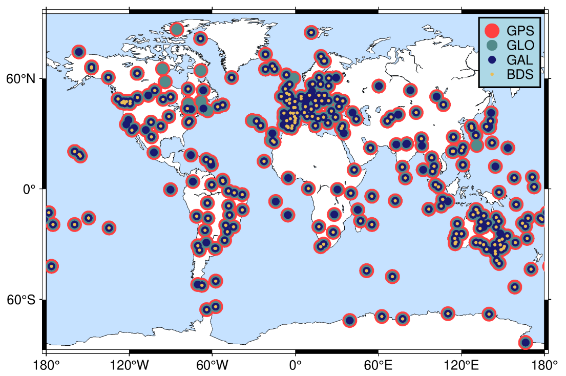
2.1. Experimental Data

In this manuscript, 364 stations are selected around the world, and their distribution is shown in Figure 1. It can be seen from the figure that almost all stations can receive GPS and GLONASS satellite signals. Due to the construction of MGEX stations in recent years, the stations supporting Galileo and BDS satellite signals are also evenly distributed worldwide. On this basis, the global ionospheric modeling strategy in this manuscript is as follows: (1) We select GPS C1W/C2W codes, GLONASS C1P/C2P codes, Galileo C1X/C5X codes, and BDS C2I/C6I codes; (2) The epoch interval of observation data is 30 s; (3) The satellite cut-off altitude angle is 7°; (4) We use a carrier phase smoothing pseudorange algorithm; (5) The order of the spherical harmonic function is 15.

The factors affecting ionospheric condition mainly include solar and geomagnetic activity. An important index to reflect the solar activity is the radioactive flux F10.7, which classifies solar activity into four levels: low, moderate, high, and very high, with boundaries of 90 sfu, 130 sfu, and 196 sfu, respectively. The geomagnetic activity mainly is measured by the Dst index, which describes the changes of the ring current during magnetic storms, the global geomagnetic disturbance index Kp index, and the interplanetary equivalent three-hour amplitude Ap index. The larger absolute value of the Dst index represents the more intense geomagnetic activity.

We show the amplitudes of solar activity and geomagnetic activity in 2021 in Figure 2. In order to study the modeling accuracy of the four systems in different conditions of the ionosphere, we select the data of 2021 and day of year (DOY) 213–242 as the experiment period, when both solar activity and geomagnetic activity are at relatively low levels; these can be referred to as the ionospheric quiet days. The data of DOY 288–317 in 2021, when the solar activity is strong and the indicators of geomagnetic activity indicate the occurrence of magnetic storms, are selected as the active ionospheric days.

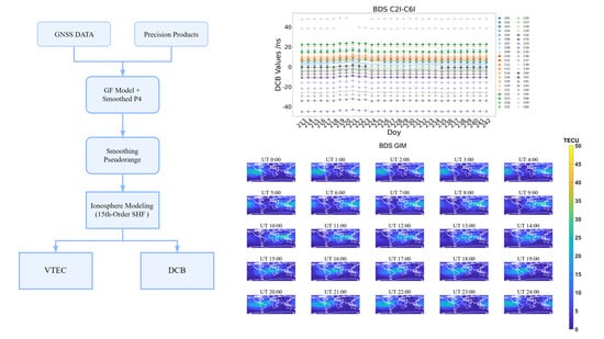
2.2. Ionospheric TEC Modeling and DCB Estimation

The approach uses the pseudrange observations and carrier phase observations from the global multi-system GNSS stations to model the global ionosphere. The observation model is as follows [44]

$$\{\begin{array}{c}{P}_{r,i}^s={\rho }_r^s+c\cdot \left(d{t}_r-d{t}^s\right)+T_r^s+I_{r,i}^s-c\cdot B_{r,i}-c\cdot B_i^s+{\epsilon }_r^s\\ {\Phi }_{r,i}^s={\rho }_r^s+c\cdot \left(d{t}_r-d{t}^s\right)+T_r^s-I_{r,i}^s-c\cdot b_{r,i}-c\cdot b_i^s+{\lambda }_i\cdot N_{r,i}^s+{\xi }_r^s\end{array}$$

(1)

where $P_{r,i}^s$ and ${\Phi }_{r,i}^s$ are code and phase measurements at frequency $i$; ${\rho }_r^s$ denotes the geometric distance from the satellite to the receiver; $c$ denotes the speed of light; $d{t}_r$ and $d{t}^s$ refer to the clock errors of the receiver and the satellite; $T_r^s$ denotes the tropospheric delay error, $I_{r,i}^s$ denotes the ionospheric delay error at frequency i; $B_{r,i}$ and $B_i^s$ are the hardware delay effects of the receiver and satellite; ${\lambda }_i$ is the wavelength at frequency $i$; $N_{r,i}^s$ denotes the carrier phase ambiguity at frequency $i$; ${\epsilon }_r^s$ and ${\xi }_r^s$ are the sum of noise and multipath effects for code and phase observations, respectively.

The pseudorange and carrier observations are combined by the geometry-free model for ionospheric delay and DCB, whose results are constructed as

$$\begin{gathered} P_4=P_{r,2}^s-P_{r,1}^s=I_{r,2}^s-I_{r,1}^s-c\left(DC{B}_r+DC{B}^s\right) \\ {L}_4=L_{r,2}^s-L_{r,1}^s=I_{r,2}^s-I_{r,1}^s-c\left(DC{B}_r+DC{B}^s\right) \end{gathered}$$

(2)

where $DC{B}_r=B_{r,2}-B_{r,1}$ and $DC{B}^s=B_2^s-B_1^s$ are the differential code biases at the receiver side and the satellite side, respectively.

In order to improve the accuracy of the pseudorange observations and not to introduce the problem of ambiguity of the carrier phase observations, we use the algorithm of carrier phase smoothing pseudorange for processing, and the equation is as follows [46]

$$\begin{gathered} P_{4,sm}={\omega }_t{P}_4\left(t\right)+\left(1-{\omega }_t\right)P_{4,prd}\left(t\right)(t>1) \\ {P}_{4,prd}\left(t\right)=P_{4,sm}\left(t-1\right)+\left[L_4\left(t\right)-L_4\left(t-1\right)\right](t>1) \end{gathered}$$

(3)

where $P_{4,sm}$ is equal to $P_4$, ${\omega }_t$ denotes the weight at epoch $t$; and $P_{4,prd}\left(t\right)$ denotes the $P_4$ forecast value. When the epoch is 1, ${\omega }_t$ is equal to 1.

When processing GNSS data, we only consider the effect of the first-order ionospheric refraction, and the effect of higher-order terms on the ionosphere is ignored. Combined with the formula $I_{r,i}^s=\frac{40.3}{f_i^2} TEC$, where $f_i$ denotes the frequency of $i$ signal, $P_{4,sm}$ can be expressed as [46]

$$P_{4,sm}=40.3\left(\frac{1}{f_1^2}-\frac{1}{f_2^2}\right)STEC+DC{B}^r+DC{B}_r$$

(4)

where the slant TEC (STEC) represents the total electron content between the satellite and the receiver. Converting Equation (4) into an expression for $STEC$ as follows [45]

$$STEC=-\frac{f_1^2{f}_1^2}{40.3\left(f_1^2-f_2^2\right)}\left(P_{4,sm}-cDC{B}_r-cDC{B}^s\right)$$

(5)

After obtaining the processed observations, we assume the ionosphere as a single-layer model in which all free electrons in the ionosphere are concentrated in a single layer at a specified height of the earth and then use the dual-frequency observations to estimate the vertical TEC (VTEC). When building the global VTEC model by the spherical harmonic function, the total electron content in the direction of the observations is estimated. We still need to convert $STEC$ by using the projection function $M\left(z\right)$ to the total electron content in the zenith direction. The ionospheric expression can be written as follows

$$VTEC=STEC\cdot M\left(z\right)={\displaystyle \sum }_{n=0}^{n_{max}}{\displaystyle \sum }_{k=0}^n\left(A_n^k\cos k{\lambda }^{\prime }+B_n^k\sin k{\lambda }^{\prime }\right)P_n^k\left(\cos {\varphi }_m\right)$$

(6)

where $n_{max}$ is the highest order of the spherical harmonic function; usually, the 15th order is chosen to meet the global modeling needs. $A_n^k$ and $B_n^k$ are the coefficients of the spherical harmonic function to be estimated. $P_n^k\left(\cos {\varphi }_m\right)$ is the Legendre function; ${\lambda }^{\prime }$ denotes the angle between the longitude of the IPP and the longitude over the geocentric-solar line; ${\varphi }_m$ denotes the geomagnetic latitude. $M\left(z\right)$ denotes the single-layer mapping function and the expression as follows [31]

$$M\left(z\right)=cos\left(arcsin\left(\frac{R}{R+H}sin\left(\alpha z\right)\right)\right)$$

(7)

where $R$ is the radius of the earth; $H$ is the height of the single-layer ionosphere model, usually taken as 350 km; $\alpha$ = 0.9782, and $z$ denotes the altitude angle of the receiver.

Combining the derivation of the above equations, we can obtain the combined expression for VTEC and DCB

$$\begin{gathered} VTEC={\displaystyle \sum }_{n=0}^N{\displaystyle \sum }_{k=0}^n\left(A_n^k\cos k{\lambda }^{\prime }+B_n^k\sin k{\lambda }^{\prime }\right)P_n^k\left(\cos {\varphi }_m\right) \\ =-\frac{f_1^2{f}_1^2}{40.3\left(f_1^2-f_2^2\right)}\left(P_{4,sm}-cDC{B}_r-cDC{B}^s\right)cos\left(arcsin\left(\frac{R}{R+H}sin\left(\alpha z\right)\right)\right) \end{gathered}$$

(8)

When the satellite and receiver DCB parameters are separated, the sum of all satellites is assumed to be zero as a constraint condition. Then, the ionospheric and DCB parameters can be estimated by the least square method.

2.3. Evaluation Methodology

We use GPS, GLONASS, Galileo and BDS to model the ionosphere, respectively. The GIM published by CODE as the reference is used for model accuracy comparison because the ionospheric modeling approach chosen for this manuscript is the same as for CODE. The $BIAS$ of statistical modeling results and reference values are used for analysis, and the expressions are as follows

$$BIAS=\frac{1}{n}{\displaystyle \sum }_{i=1}^n\left(TE{C}_{ref}-TE{C}_{cgs}\right)$$

(9)

where $TE{C}_{ref}$ denotes the value of the reference GIM, $TE{C}_{cgs}$ is the value solved in this manuscript, and $n$ is the number of parameters.

3. Results and Analysis

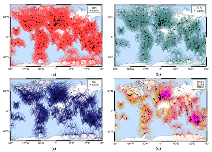
3.1. IPP Distribution

We plot the 24-h IPPs distribution DOY 212, 2021 to analyze the global ionospheric modeling performance of the four systems, and the results are shown in Figure 3. It can be seen that the IPPs of GPS are the densest among the four systems, covering most of the global land area. Moreover, the IPPs are sparse only in the polar region and oceanic region. Although the number of IPPs of GLONASS is less than that of GPS, the coverage area is similar to that of GPS. The distribution of Galileo IPPs is similar to that of GPS and GLONASS, basically covering most of the mainland. The BDS-2 and BDS-3 are plotted separately. As can be seen from Figure 3, BDS-2 mainly serves the Asia-Pacific region and Europe, while BDS-3 has the ability to provide global services, and the number of IPPs has increased significantly compared with BDS-2. The spatial distribution characteristics of BDS IPPs are similar to other systems, basically covering the global continents.

BDS has three different types of orbiting satellites, including 27 MEO satellites, 10 IGSO satellites and 8 GEO satellites. Those three types of satellites have different characteristics because of their orbit design. MEO orbits are at an altitude of about 21,528 km, and the MEO IPPs trajectory are continuous arcs. GEO orbits are at an altitude of about 35,786 km above the Earth’s equator; they remain relatively stationary from the ground, and GEO IPPs are theoretically a point. IGSO orbits are at an altitude of about 35,786 km, and the IGSO IPPs have a trajectory shaped like “8” because of the angle between the orbital plane and the equatorial plane. In this manuscript, three types of orbiting satellite IPPs are mapped, as shown in Figure 4. MEO IPPs are the most widely distributed owing to the BDS MEO satellite, which enables global coverage and global service capabilities. The IGSO servant region is the Asia-Pacific region; thus, the IGSO IPPs are mainly located in the Asia-Pacific region. Furthermore, since IGSO signals can also be received in parts of the European region, there are a lot of IPPs in the European region pictured, and the openings in the IGSO IPPs trajectory are eastward. The GEO satellites are stationary near the equator, and GEO IPPs are mainly located in the Asia-Pacific and European regions. New data resources for global ionospheric modeling could be made available by the abundance of orbital resources of BDS.

3.2. Validation of Ionosphere Estimation Algorithm

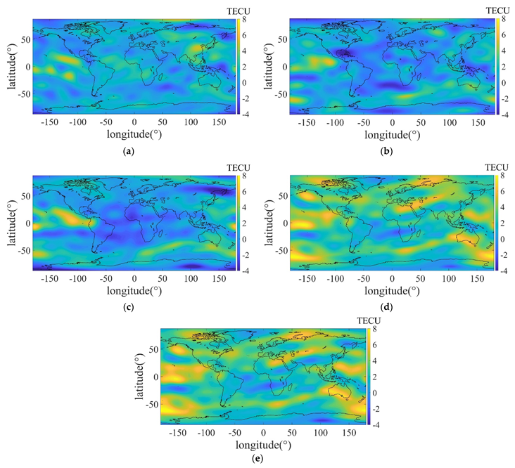
3.2.1. Accuracy of Ionosphere Model in Quiet Day

In order to test the accuracy of the ionospheric model established by the four systems, we compare the GIMs established by GPS, GLONASS, Galileo and BDS with the CODE GIMs as the reference. Due to the orbital characteristics of GEO satellites, BDS is divided into two groups to study the contribution and role of BDS GEO satellites: one is composed of three orbital satellites, MEO + IGSO + GEO, labeled as BDS; the other group only consists of MEO + IGSO and is labeled as BDS (MEO + IGSO).

Figure 5 shows the biases between the results and CODE GIM at UT 0:00 DOY 213 in 2021. As can be seen from the figure, the ionospheric biases modeled by using GPS or GLONASS are better than 2 TECU compared to CODE GIM. The larger biases are mainly in the areas where the stations are sparse and located close to the spot of direct sunlight. The similarity between GPS and GLONASS models is mainly due to the similar numbers of IPPs. The ionospheric model developed by Galileo has biases of up to 6 TECU compared to 4 TECU in most regions of CODE GIM, and the largest difference mainly exists in the ocean and polar regions. The model accuracy is slightly lower than that of GPS and GLONASS because of the few IPPs of Galileo and the lack of receivers for receiving Galileo signals in regions with large biases. Although the maximum biases between the ionospheric model developed by BDS and CODE GIM are up to 8 TECU, the biases in most regions are within 6 TECU. BDS has a global service capability but has fewer receivers that can receive BDS signals, resulting in the lowest number of IPPs in the four systems in global ionospheric modeling, affecting the accuracy of ionospheric modeling. The accuracy of the BDS (MEO + IGSO) ionosphere model is similar to BDS but slightly lower in the Asia-Pacific region, which is due to the fact that BDS GEO satellites can be observed at most stations in the Asia-Pacific region, and the number of Asia-Pacific region IPPs is greatly increased.

We analyze the results of the GIMs average biases at different latitudes between four systems and CODE GIMs during the ionospheric quiet day, as shown in Figure 6. Figure 6 shows that the biases between CODE GIMs and GIMs of the four systems established in DOY 213–242 in 2021 for northern hemisphere high latitude (NH) (60°N–90°N), northern hemisphere middle latitude (NM) (30°N–60°N), northern hemisphere low latitude (NL) (0°–30°N), southern hemisphere low latitude (SL) (0°–30°S), southern hemisphere middle latitude (SM) (30°S–60°S), and high-southern hemisphere (SH) (60°S–90°S). The results show the similar modeling performance for GPS, GLONASS and Galileo, and the average biases between GPS, GLONASS and Galileo GIMs and CODE GIMs are within 2 TECU. The biases of the BDS ionospheric model are 0–4 TECU larger than those of the other systems, and the biases in the southern hemisphere are smaller than those in the northern hemisphere. In addition, the modeling performance of BDS and BDS (MEO + IGSO) is similar, and the biases between them are in the range of 1 TECU. There are some differences between the high-latitude region of the northern hemisphere and the middle latitude region of the southern hemisphere owing to GEO satellites mainly serving the Asia-Pacific region and enriching the number of IPPs in this region.

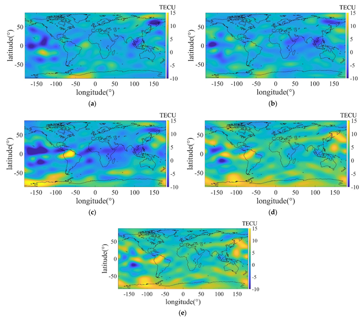
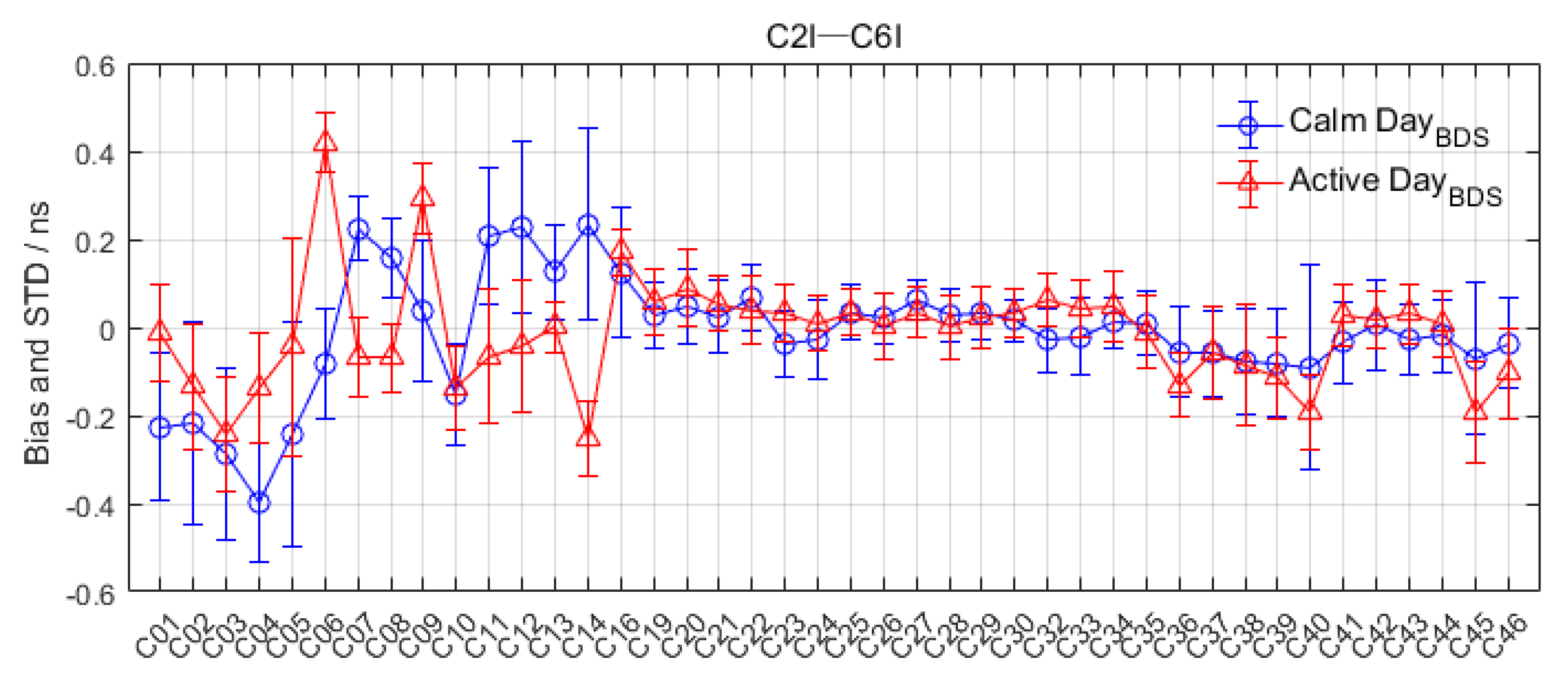
3.2.2. Accuracy of Ionosphere Model in Active Day

This manuscript selects DOY 288–317 in 2021 for ionospheric modeling and analyzes the modeling accuracy of the four systems in the active state of the ionosphere. Figure 7 shows the biases distribution between the modeling results of the four systems at DOY 308 UT 0:00 and the CODE GIMs. It can be seen from the figure that the ionospheric bias values range increases around 7 TECU during active days compared with GIMs in calm days. The places with large biases between the ionospheric models established by the four systems mainly exist in the equatorial region and polar regions west of the 0-degree longitude. The ionosphere is more active in the equatorial region of west of the 0-degree longitude due to the stronger solar radiation during the day. The reason for the larger biases in the polar regions is that the region is affected by the combined effects of solar radiation and geomagnetic storms.

Among others, the biases between the models established by GPS and GLONASS are in the range of 5 TECU, and the biases become larger at about 10 TECU in the ocean and polar regions. The biases between GPS and GLONASS are relatively small among the four systems owing to the number of stations being large and the global distribution being even. The Galileo ionospheric model’s biases are less than 10 TECU in most land areas, and the ocean and polar regions are affected by solar radiation and geomagnetic storms where the biases are obviously located near the equator, with the largest bias reaching 15 TECU. The biases of the BDS ionospheric model are in the range of 10 and 15 TECU; especially, the biases in polar and oceanic regions are more than 10 TECU. Moreover, the biases do not change significantly after adding GEO satellites.

Figure 8 shows the average biases from the CODE GIMs at different latitudes for the four systems in the active condition of the ionosphere during DOY 288–317 in 2021. The GPS, GLONASS and Galileo average biases from CODE GIMs are within 2.5 TECU. The biases of the BDS ionospheric model are significantly smaller in the mid-latitude and high-latitude regions of the northern hemisphere than those of in the southern hemisphere. The biases in the northern hemisphere are basically stable within 4 TECU, while the biases in the southern hemisphere are in the range of 4–8 TECU. The biases in the southern hemisphere are the largest, and the main reason is that there are fewer stations in the high and mid-latitude regions of the southern hemisphere, resulting in less IPPs than the northern hemisphere. The biases of the BDS ionospheric model are larger in low latitudes with 2–8 TECU, which is mainly caused by the enhanced solar radiation and the small number of BDS IPPs. Comparing the model biases of BDS and BDS (MEO + IGSO), it can be seen that the biases between the two GIMs in the ionospheric active condition are also in the range of 1 TECU. It may be concluded that GEO has less influences on the ionospheric modeling in the ionospheric active condition.

3.2.3. Analysis of Ionospheric Outliers

In the process of ionospheric modeling, TEC values are negative in some grid points, which is due to the absence of observations and a few number of IPPs. In order to avoid the negative value of TEC, we reference the method of the CODE Analysis Center, set the negative value of the grid points as 0 and mark these values as 0-value [47]. To study the influence of 0-value in the ionosphere modeling, the global distribution map of 0-value in the ionosphere of four systems is drawn, and the results are shown in Figure 9. It can be seen from the figure that the four systems have large 0-value regions in the southern hemisphere, especially in the Antarctic region. This condition is mainly owing to the number of stations in this region being small, and therefore, it is difficult to obtain sufficient observations. In the middle and high latitudes of the northern hemisphere, GPS and BDS also have some 0-value regions; however, the area is much smaller than the area of the southern hemisphere. Among others, the area of 0-value of BDS is the largest among the four systems because few receivers receive BDS signals in polar regions and surrounding regions, and there is an insufficient number of IPPs. Significantly, BDS (MEO + IGSO) has a large region of 0-value globally, and the improvement of performance is not obvious even after the GEO satellite is added. To further investigate the influence of the 0-value at different latitudes, we add up the number of 0-value points for each hour in a month and calculate the mean number of 0-value in an hour according to different latitudes. The results are shown in

Table 1. The mean number of each system 0-value in different areas during ionosphere quiet days (DOY 213–242 in 2021).

Area	GPS	GLONASS	Galileo	BDS	BDS (MEO + IGSO)
NH	0.05	1.32	6.78	40.36	42.22
NM	0.01	1.08	8.38	49.83	45.06
NL	0.10	0.13	0.17	5.08	4.67
SL	0.04	0.12	3.42	22.8	30.24
SM	82.97	114.31	156.99	328.87	406.42
SH	233.93	217.96	346.6	691.72	680.57

.

As can be seen from Table 1, only a few 0-values of GPS are in the northern hemisphere and thus can be ignored. In the southern hemisphere, there are some 0-values of GPS in the low and middle latitudes, about 0.04 and 82.87 in an hour, respectively. A large number of 0-value areas are in the high latitudes of the southern hemisphere, about 233.93 in the region. The main reason that affects the 0-value grid points is the absence of observations and the few IPPs. Combined with Figure 3 and Figure 9, it can be seen that the 0-values of these two regions are distributed in the ocean and polar regions with a small number of stations. Due to the sparse stations, these regions have less IPPs and observations. The 0-value of GLONASS is found in the middle and high latitudes of the southern hemisphere, about 114.31 and 217.96, respectively. The numerical characteristics and spatial distribution characteristics of 0-values in Galileo are similar to GLONASS in that the number of 0-values in the middle latitudes is less than that in the high latitudes. The number of 0-values of BDS owns the largest among the four systems, and the 0-values exist in all latitude regions. That is because the number of receivers that can receive BDS signals is less than the other three systems, the number of satellites that can be observed varies from region to region, and the number of IPPs is less than the other systems. In addition, by comparing the results of BDS and BDS (MEO + IGSO), we can see that GEO satellites do not play an obvious role in ionospheric modeling, because compared with the MEO and IGSO, IPPs of GEO are only points or small circles, and the number and spatial scope are greatly limited. Moreover, the orbital inclination of the satellites also has influences, the orbital inclination of GPS and BDS (MEO and IGSO) is 55°, and that of GLONASS is 64.8°and that of Galileo is 56° [12,48]. Thus, GLONASS performs better than others in high latitudes of the southern hemisphere. It is worth noting that the number of satellites IPPs and 0-value region are variable as the visibility of the satellite changes. In this manuscript, GPS performs better than Galileo in most cases, and Figure 9 only shows the result of 0-value in one hour for manuscript length.

Figure 10 shows the distribution of the four systems 0-value regions at DOY 308 UT 0:00 in 2021, and

Table 2. The mean number of each system 0-value in different areas during ionosphere active days (DOY 288–317 in 2021).

Area	GPS	GLONASS	Galileo	BDS	BDS (MEO + IGSO)
NH	0.66	1.33	2.69	59.96	59.86
NM	0.47	1.62	2.78	51.02	52.65
NL	0.04	0.11	0.13	3.22	2.70
SL	0.01	0.00	0.24	10.49	13.89
SM	15.23	14.81	17.67	113.58	139.07
SH	12.23	11.54	21.94	187.99	169.41

shows the mean number of 0-value at different latitudes during the ionospheric active days. As can be seen, the 0-value regions of all four systems are significantly reduced compared to the quiet day, especially in the high latitudes of the southern hemisphere, where the mean 0-value number of GPS and GLONASS is less than 20, that of Galileo is less than 50, and that of BDS is less than 200. This result is better than that of the quiet days because in active days, the number of total electron content changes rapidly and reduces the number of 0-value. Normally, on quiet days, the total electron content in high latitude is much smaller than that in low latitude.

However, on ionosphere active days, the arctic region is in polar night and south pole is in polar day, which is different from quiet days. There are many unique physical phenomena in the polar region, and using expressions cannot accurately describe the ionospheric changes sometimes. Future research should certainly test whether these orbital factors can influence the number of 0-value.

3.3. Validation of DCB Estimation Algorithm

DCB represents the signal time delay between the codes of different frequencies and types. Due to the fact that DCB and TEC are coupled to each other, the stability and accuracy of DCB is also one of the important indicators for evaluating the ionospheric model. Therefore, we evaluate and analyze the satellite DCB of four systems.

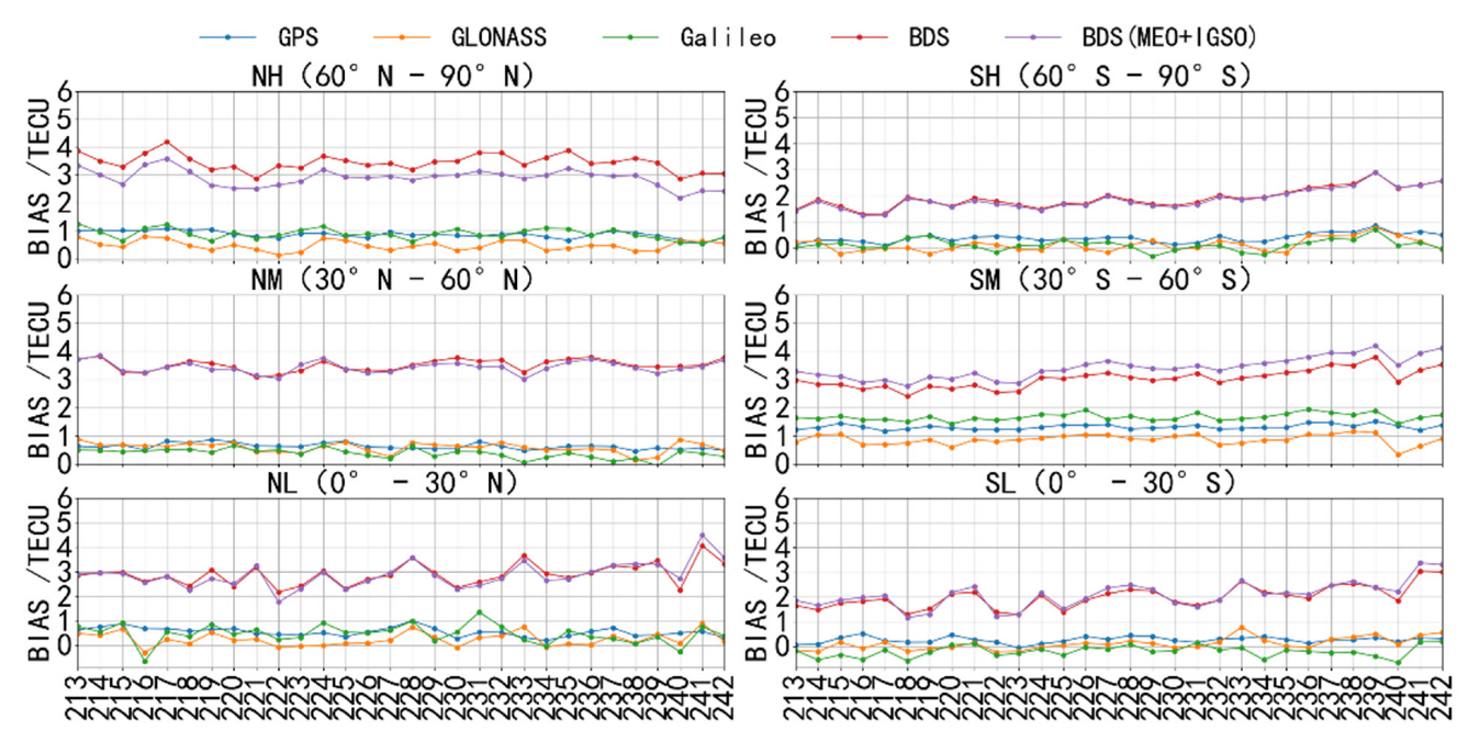
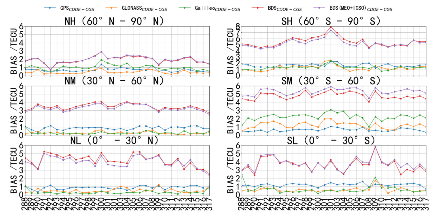
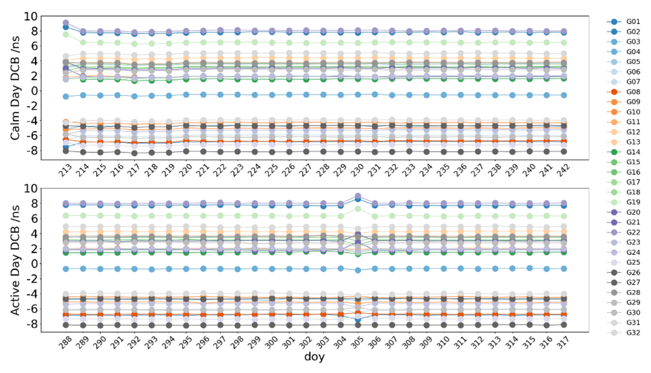
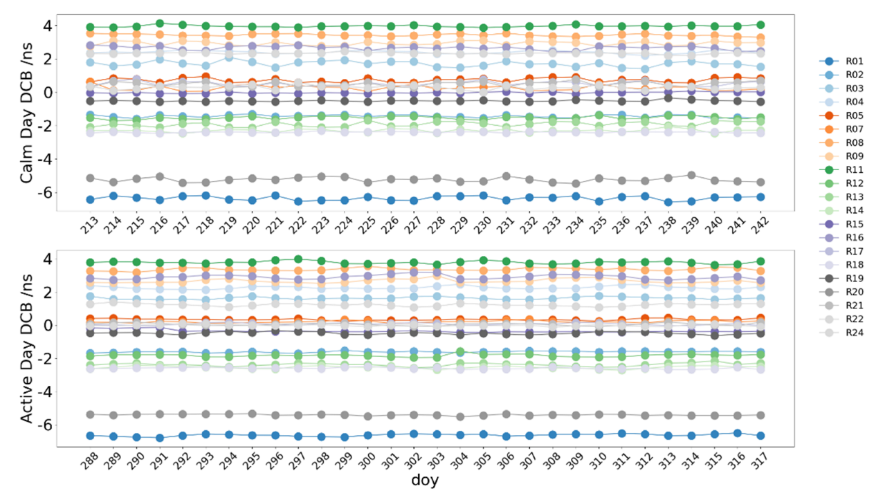
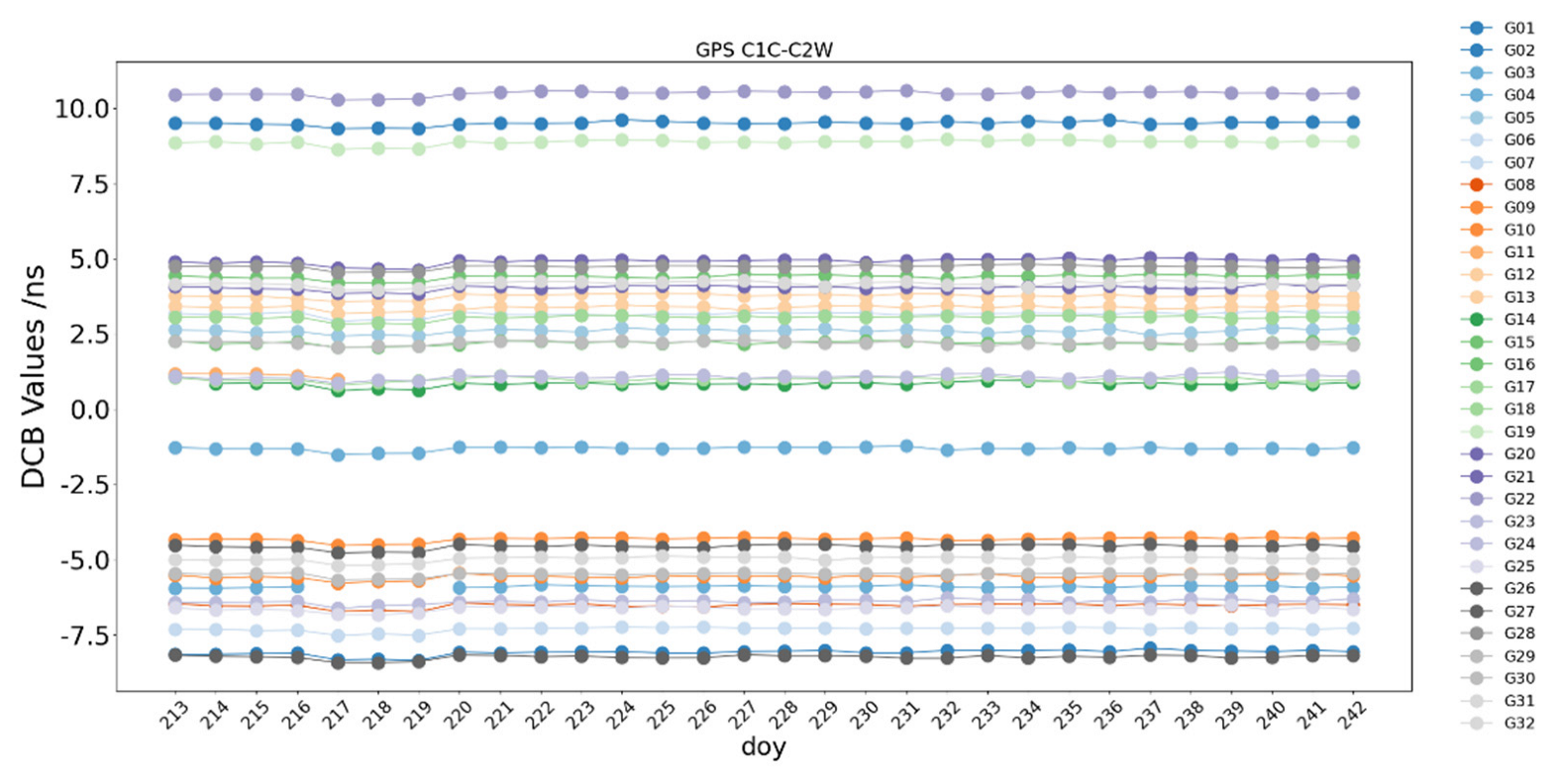
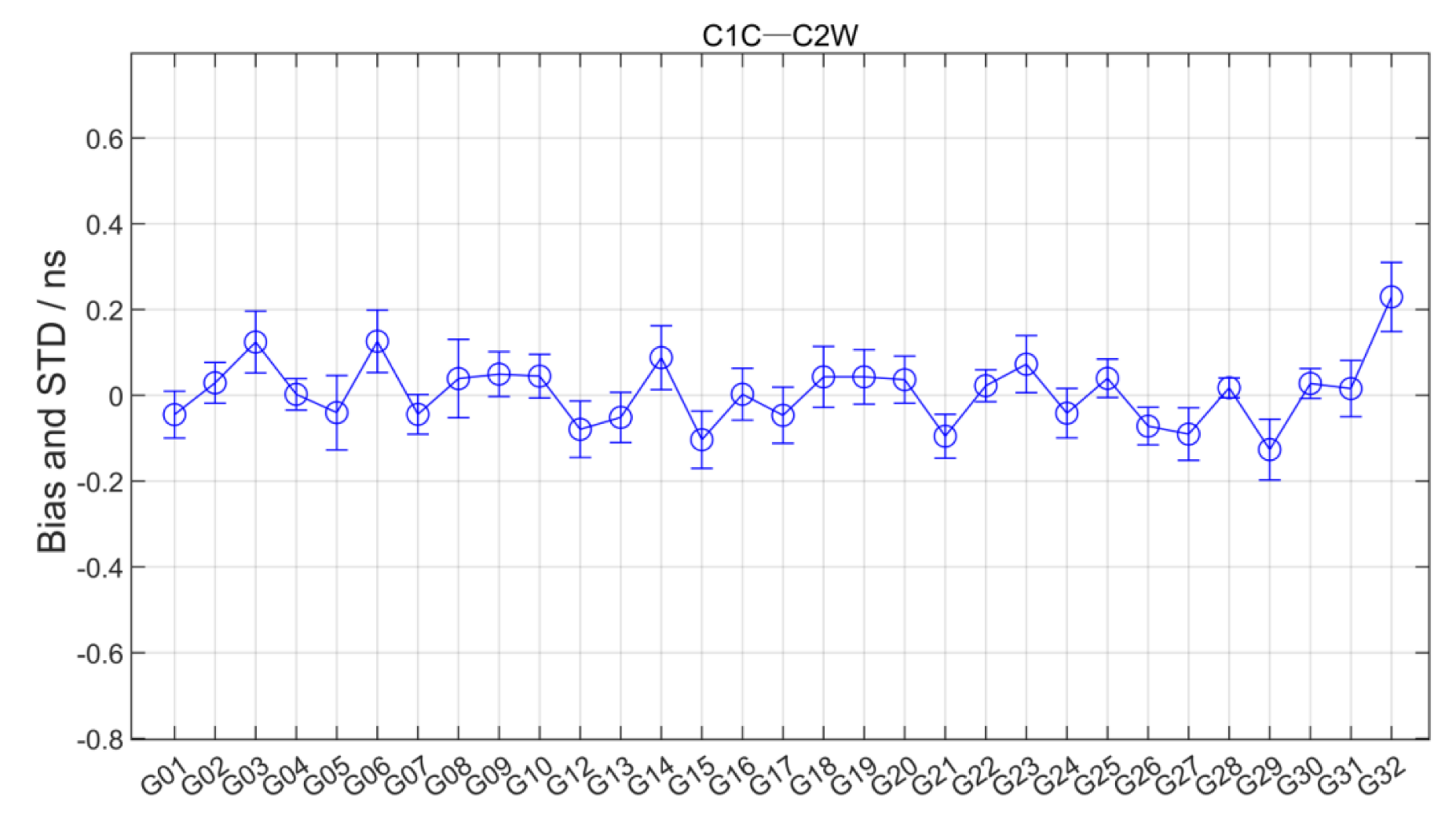
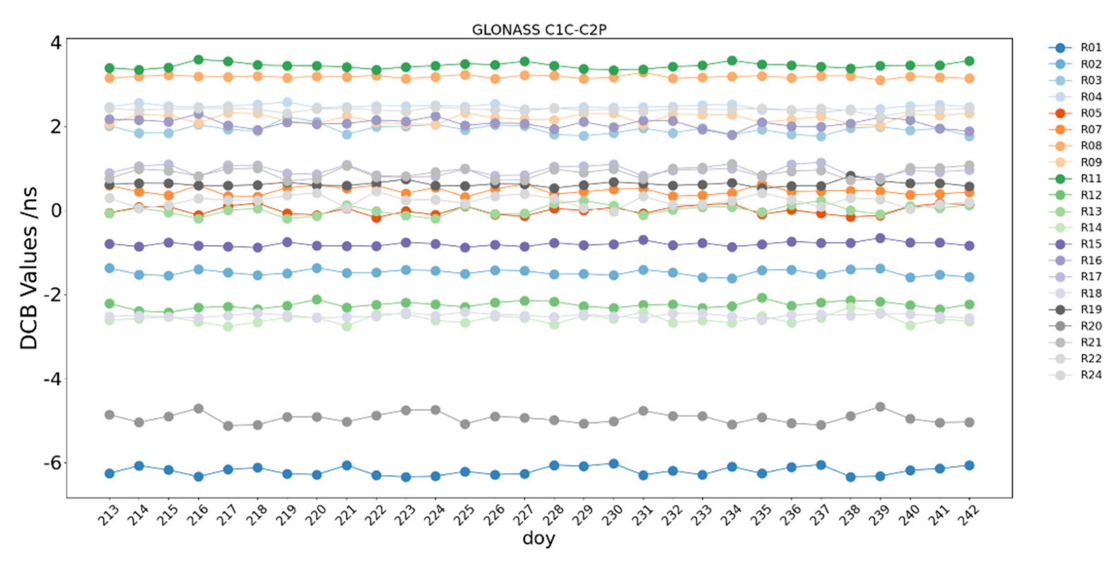
3.3.1. Accuracy of GPS and GLONASS DCB

Figure 11 and Figure 12 show the time series of GPS satellite C1W–C2W DCB and GLONASS satellite C1P-C2P DCB at different ionospheric conditions, respectively. It can be seen from the figure that the DCB of GPS and GLONASS satellites shows strong stability during the 30 days and are less affected by the ionosphere. In order to verify the outer precision of the estimated DCB, we compare the estimated results with the DCB products published by CODE, and the results are shown in Figure 13 and Figure 14. It can be seen from the figure that GPS and GLONASS are consistent to each other. The average biases of DCB of all satellites is within 0.25 ns, and STD is basically within 0.1 ns.

3.3.2. Accuracy of Galileo DCB

Since CODE DCB products of Galileo and BDS are not provided, we select Galileo DCB and BDS DCB of CAS for comparative analysis. Figure 15 shows the time series of Galileo satellite C1X-C5X DCB estimated in this manuscript during the quiet and active ionospheric days. It can be seen that Galileo satellite DCB has strong stability, and the values of DCB are basically in the range of 0.2 ns. Figure 16 shows the average biases and STD of Galileo with CAS DCB products. The estimated average biases and STD of Galileo satellite DCB results with CAS DCB are in the range of 0.2 ns, presenting a good consistency.

3.3.3. Accuracy of BDS DCB

Figure 17 shows the time series of C2I-C6I DCB of BDS during the ionospheric quiet days and active days, where the upper is the MEO and IGSO satellite of BDS, and the lower is the GEO satellite. It can be seen from the figure that the satellite DCB values of BDS are in the range of 50 ns. Among others, the BDS GEO satellite DCB often disappeared, because the observations of GEO are less stable than those of MEO and IGSO. If the ephemeris were missing or the corresponding satellite was marked unhealthy, the satellite DCB also cannot be estimated. In addition, the IGSO DCB estimated in this manuscript also disappeared because of the lack of navigation data. As can be seen from the figure, when the satellite DCB has disappeared, the other satellite DCB values have an obvious change. This is because when separating the satellite DCB and receiver DCB parameters, the sum of all satellite DCB is 0 for constraint. When the satellite is missing, the benchmark of the satellite will change.

Figure 18 shows the average biases and STD of estimated BDS DCB and CAS products during quiet and active days. It can be seen from the figure that the average biases of DCB of BDS-2 are within 0.42 ns, while those of STD are within 0.25 ns. BDS-3 average biases are within 0.2 ns, and those of STD are within 0.25 ns; therefore, the consistency of BDS-3 is better than that of BDS-2. In addition, since DCB of C59 and C60 satellites are not provided in CAS DCB products, these two satellites are not counted in the statistical process in this manuscript.

3.3.4. Accuracy of Other Frequency DCB Type

In order to verify the stability and accuracy of other codes DCB, we use the ionosphere results of GPS as a constraint to estimate other DCB types of each GNSS system. In this part, we select GPS C1C/C1W codes, GLONASS C1C/C2P codes, Galileo C1C/C5Q codes and BDS C2I/C7I codes.

Figure 19 shows the time series of GPS satellite C1C–C2W DCB. It can be seen that the DCB of GPS shows strong stability in the month. We compare the result with CAS DCB products. As is shown in Figure 20, all satellite average DCB biases are within 0.4 ns, and the STD is basically within 0.1 ns, which performs worse than C1W–C2W.

Figure 21 shows GLONASS satellite C1C–C2P DCB time series, and Figure 22 shows the biases and STD of the DCB compared with CAS. The results show C1C–C2P DCB is stable, the average DCB biases are within 0.3 ns, and the STD is within 0.2 ns, which performs worse than C1P–C2P.

Figure 23 shows Galileo satellite C1C–C5Q DCB time series, which is similar to C1X–C5X performance. Figure 24 shows the average biases and STD of Galileo with CAS DCB products. The estimated average biases and STD of Galileo satellite DCB results with CAS DCB are in the range of 0.2 ns, presenting a good consistency.

We estimated C2I–C7I DCB in order to verify the BDS-2 performance. The result is shown in Figure 25 and Figure 26. BDS-2 has five GEO(C01~C05), seven IGSO (C06~C10, C13 and C16) and three MEO (C11, C12 and C14) satellites. Compared with C2I–C6I DCB, C2I–C7I DCB is less stable and shows discontinuity, especially with GEO and IGSO satellites. The estimated average biases of the satellite DCB is within 0.6 ns and the STD is about 0.2 ns, which performs worse than C2I–C6I. Thus, we select C2I–C6I codes to ionosphere modeling, which has the advantage of more satellites and a high accuracy of measurement codes.

Based on the above results, we can see that although these types DCBs perform worse than those used in ionospheric modeling, it is still acceptable. Thus, other combinations of codes can be considered for ionospheric modeling in future studies.

4. Discussion

We compare and analyze the performance of the four systems in ionospheric modeling since GNSS has entered a new stage, especially as the BDS-3 completed its constellation in July 2020. The results show that the ionospheric modeling performance of GPS, GLONASS and Galileo is comparable, while the BDS still needs to be improved. In addition, with the improvement of precise products such as orbit and clock biases and improved models, the accuracy of the BDS ionospheric model will be further improved. We use ionosphere results as a constraint to estimate the other DCB types of each GNSS system. The result also verifies the results of ionosphere models in this manuscript.

We also analyze the characteristics of the ionospheric outliers and attribute them to the distribution of the stations. In this manuscript, we only show the ionospheric outliers at time 0:00 in the experimental data owing to the limitation of the space. In fact, the area of 0-value where outliers appear is not constant. The outliers may appear when there are not enough observations at the stations in a time period or when the quality of the observations is bad. In addition, the interpolation method used in the modeling also leads to the occurrence of outliers. Considering the unique physical phenomena that occur in the ionosphere, especially polar day and night in polar regions, and during ionosphere active days, the number of total electron content changes rapidly. Using expressions cannot accurately describe ionospheric changes sometimes. Thus, the number of 0-value is influenced by many factors. Future research should certainly test whether these orbital factors can influence the number of 0-value. The results of ionospheric modeling using the BDS single system show that GEO satellites do not cause significant differences. It is also worth noting that the BDS-3 DCB outperforms that of BDS-2, and the larger BDS-2 DCB and the instability of the GEO satellite DCB may also be responsible for the higher number of BDS ionospheric outliers, which should be considered in subsequent studies. In future studies, the characteristics of ionospheric modeling changes over short periods of time, such as satellite visibility, IPPs and outliers in the ionosphere over multiple time periods, should also be investigated to analyze the intrinsic relationships.

5. Conclusions

Based on the data from 364 globally distributed stations, we use the 15-order spherical harmonic function algorithm to estimate the ionospheric model of GPS, GLONASS, Galileo and BDS, respectively. The performances of the four systems in the ionospheric quiet and active conditions are compared and analyzed. The accuracy of the ionospheric by-product DCBs is analyzed and evaluated. The results show that:

• The IPPs of GPS and GLONASS are abundant and globally distributed. With the construction and development of Galileo and BDS, Galileo and BDS IPPs cover the global continents. However, Galileo and BDS IPPs are less than that of GPS and GLONASS, which is mainly due to the limited number of stations.
• GPS and GLONASS ionospheric models with greater accuracy, followed by Galileo. Although BDS is limited by the number of stations and has the lowest number of IPPs of the four systems, the ionospheric model built still performs well.
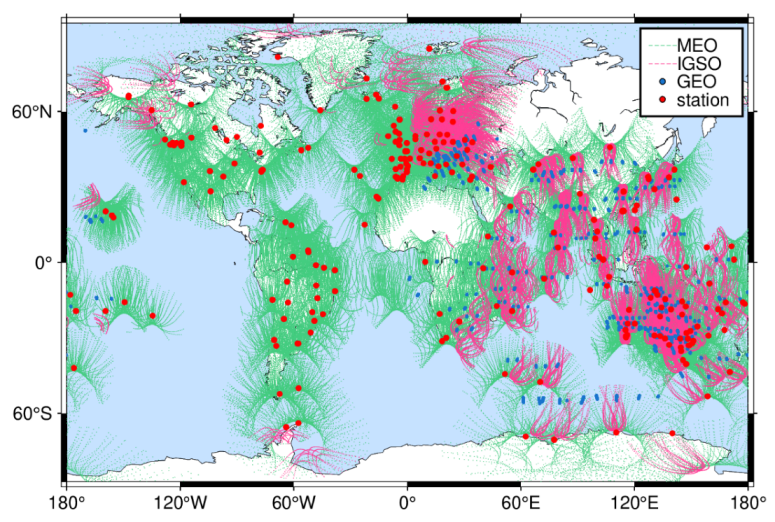
• The orbit characteristics of the BDS GEO satellite make its IPPs a point above the earth. When IPPs are abundant, it does not play an obvious role in ionosphere modeling.
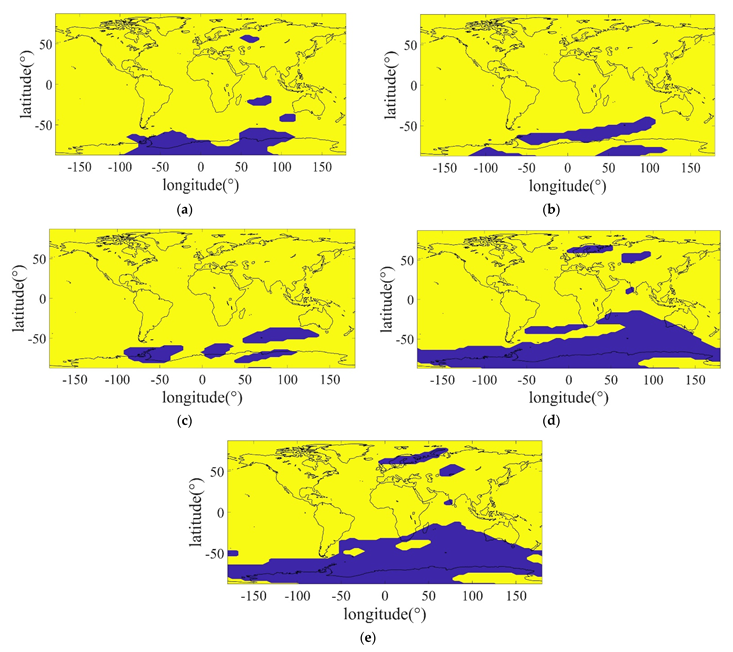
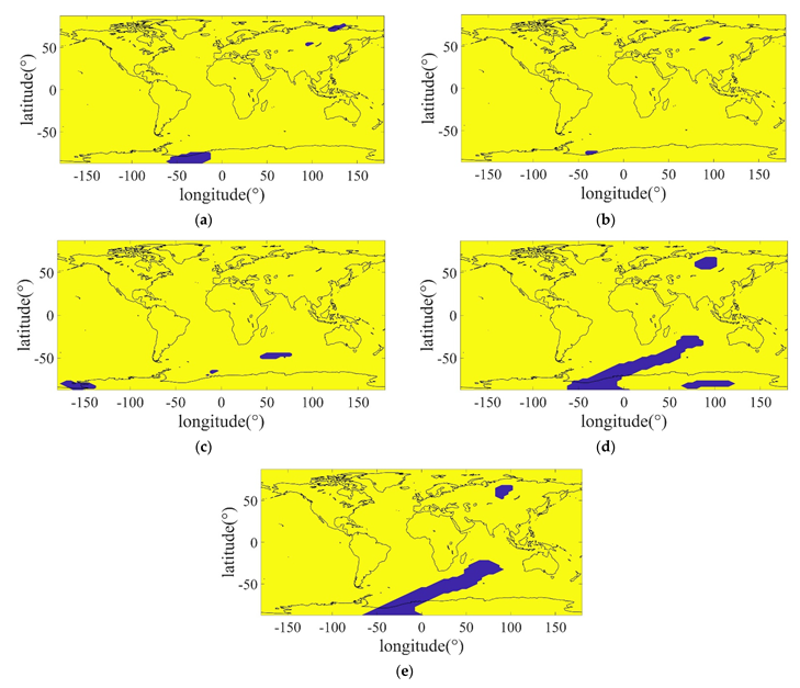
• Some grid points will be negative in the ionospheric modeling results, which will be assigned as 0 in this manuscript, and the number and proportion at the latitude will be counted. The 0-value region is mainly distributed in the middle and high latitude regions of the southern hemisphere. The 0-value area of BDS is larger than that of the other systems.
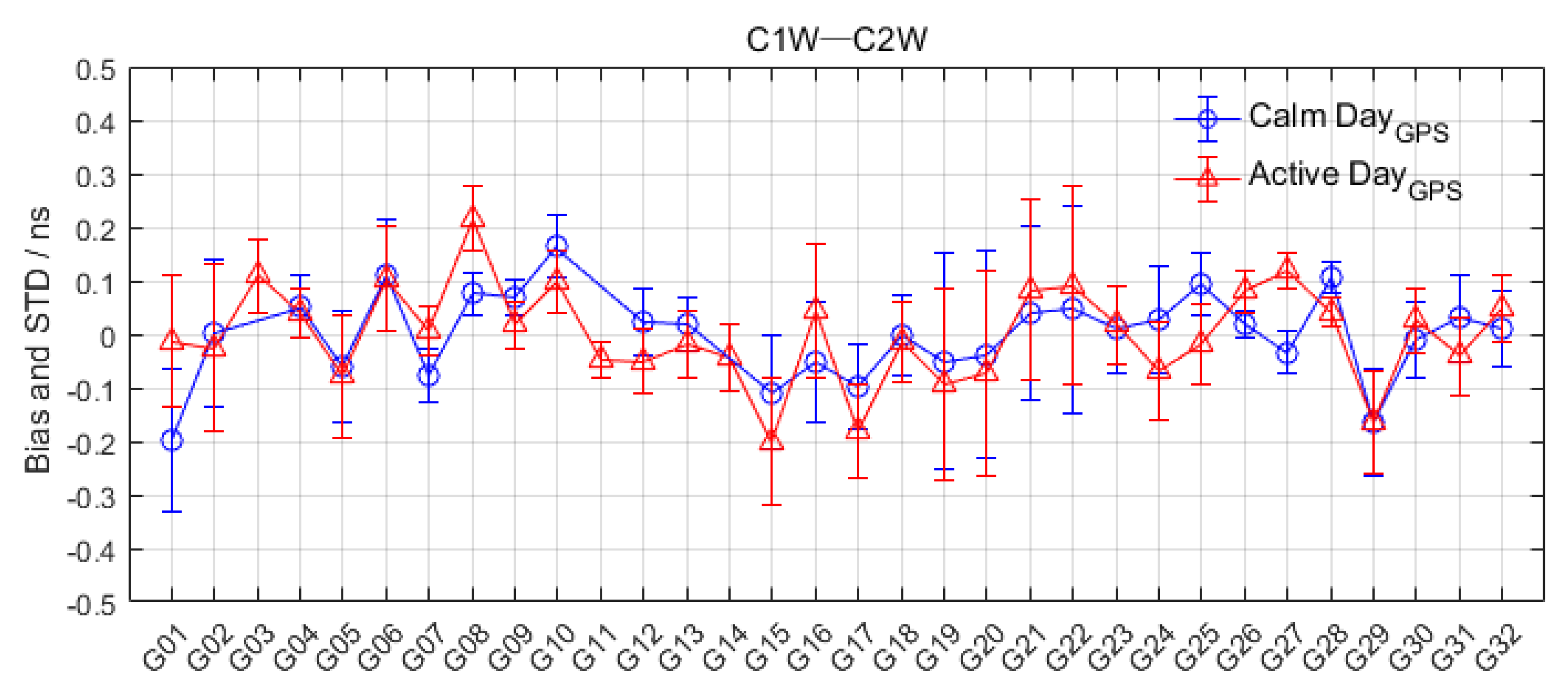
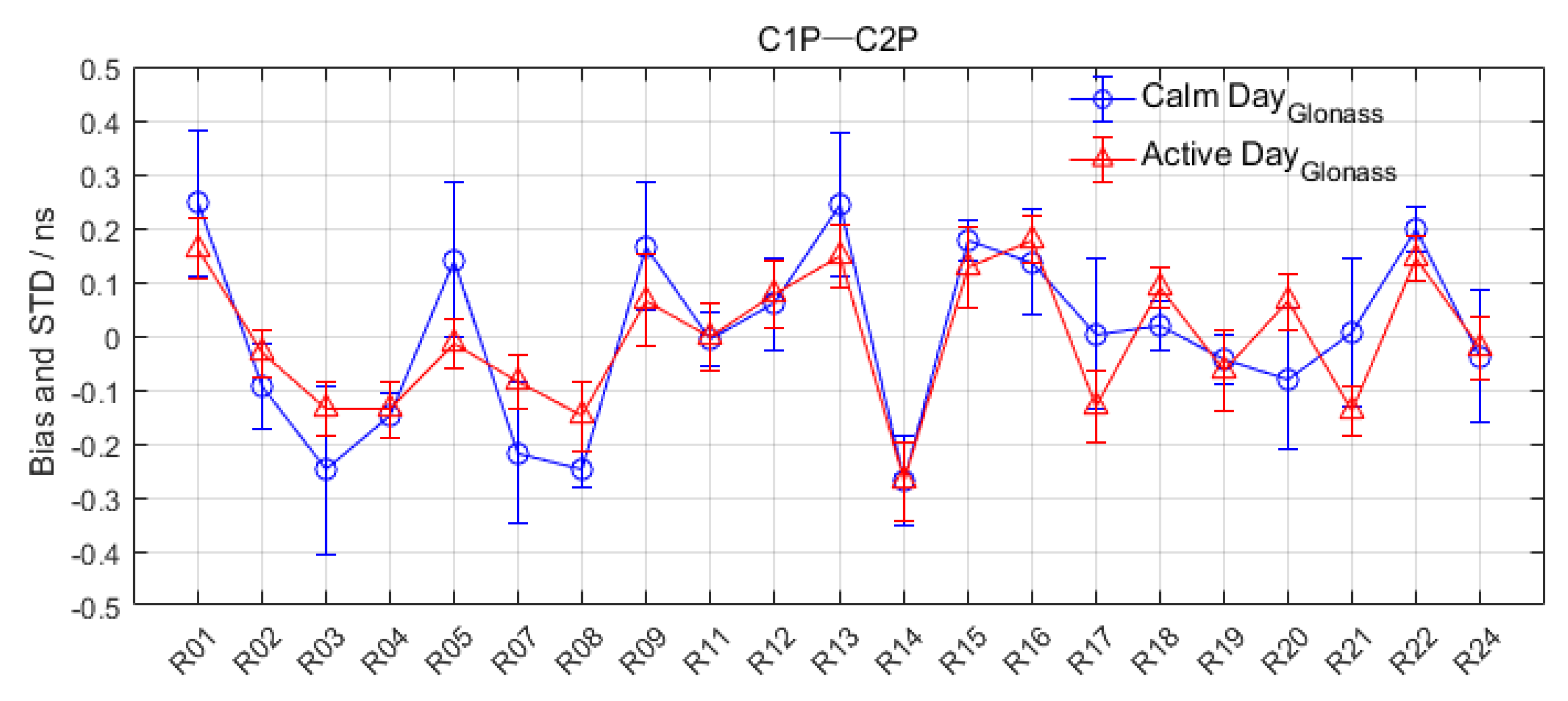
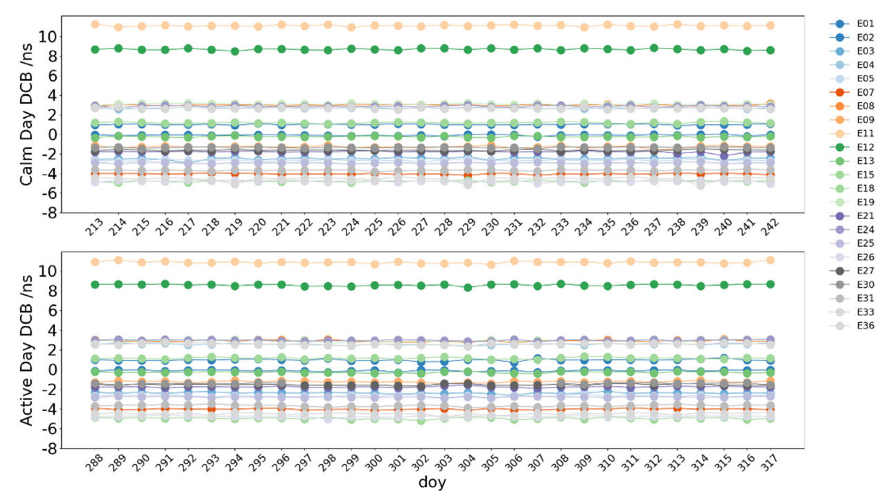
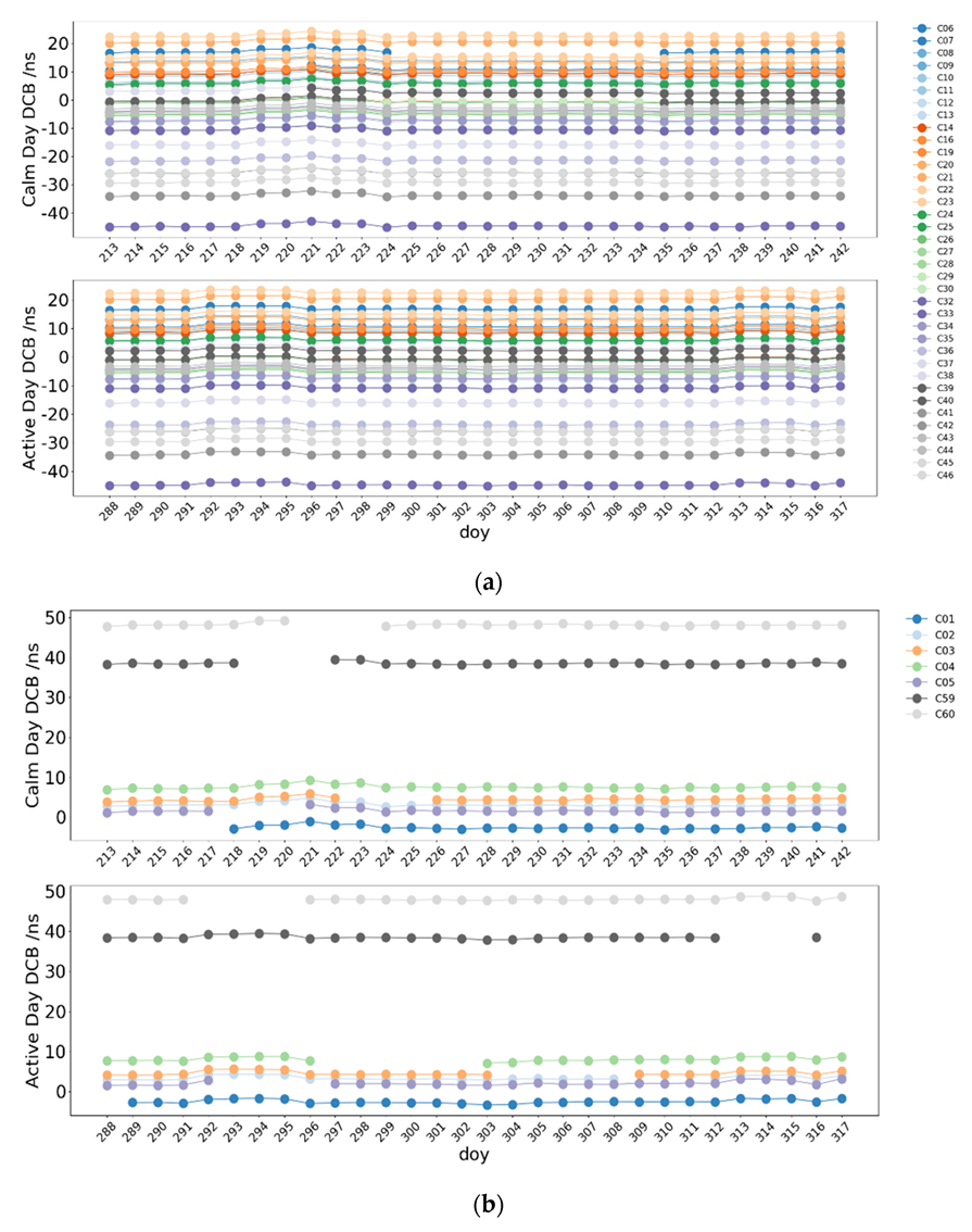
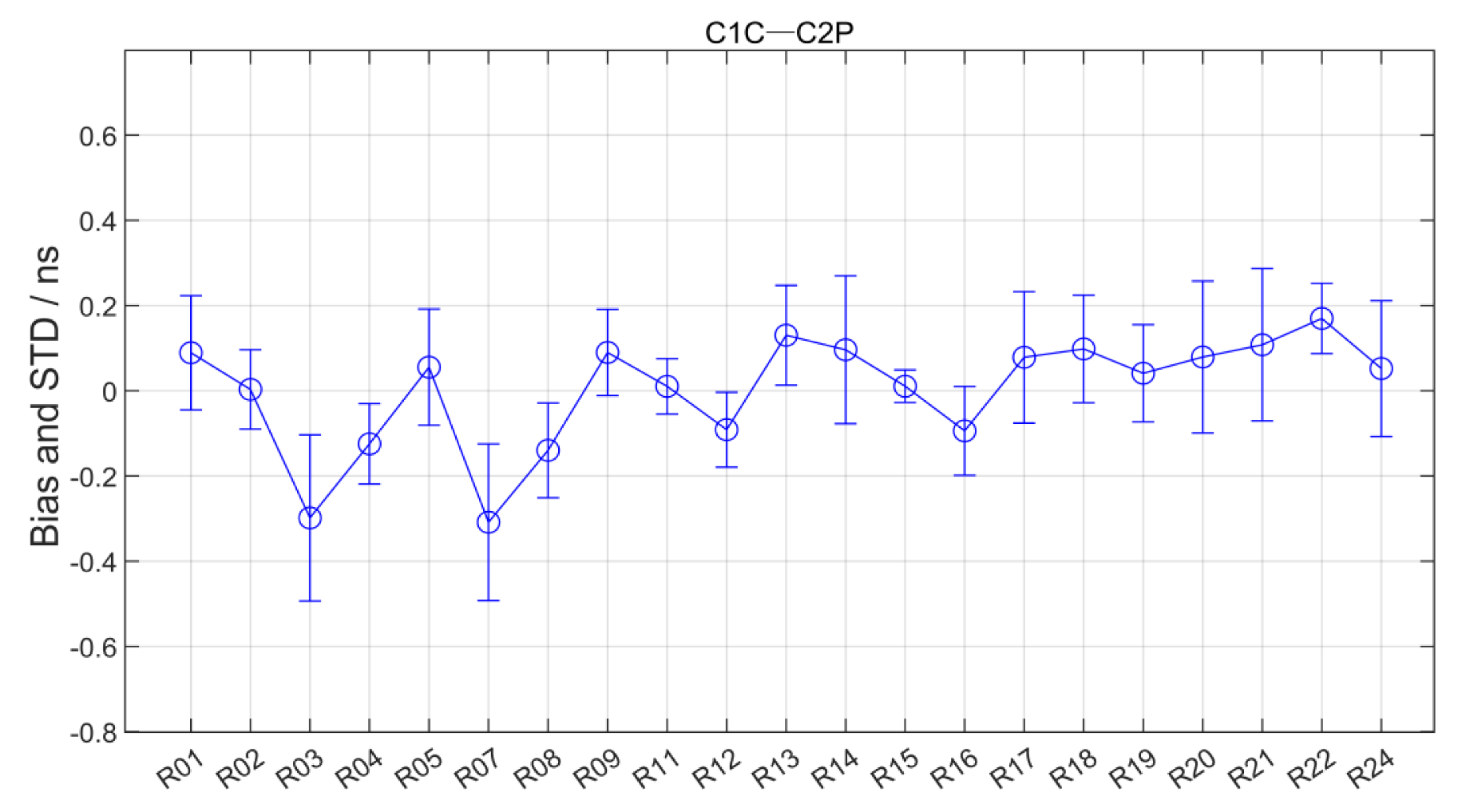
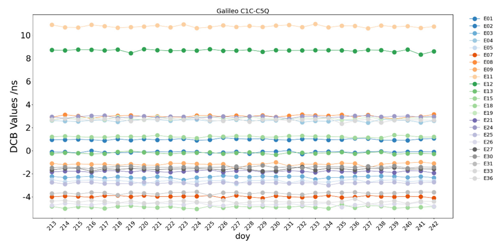
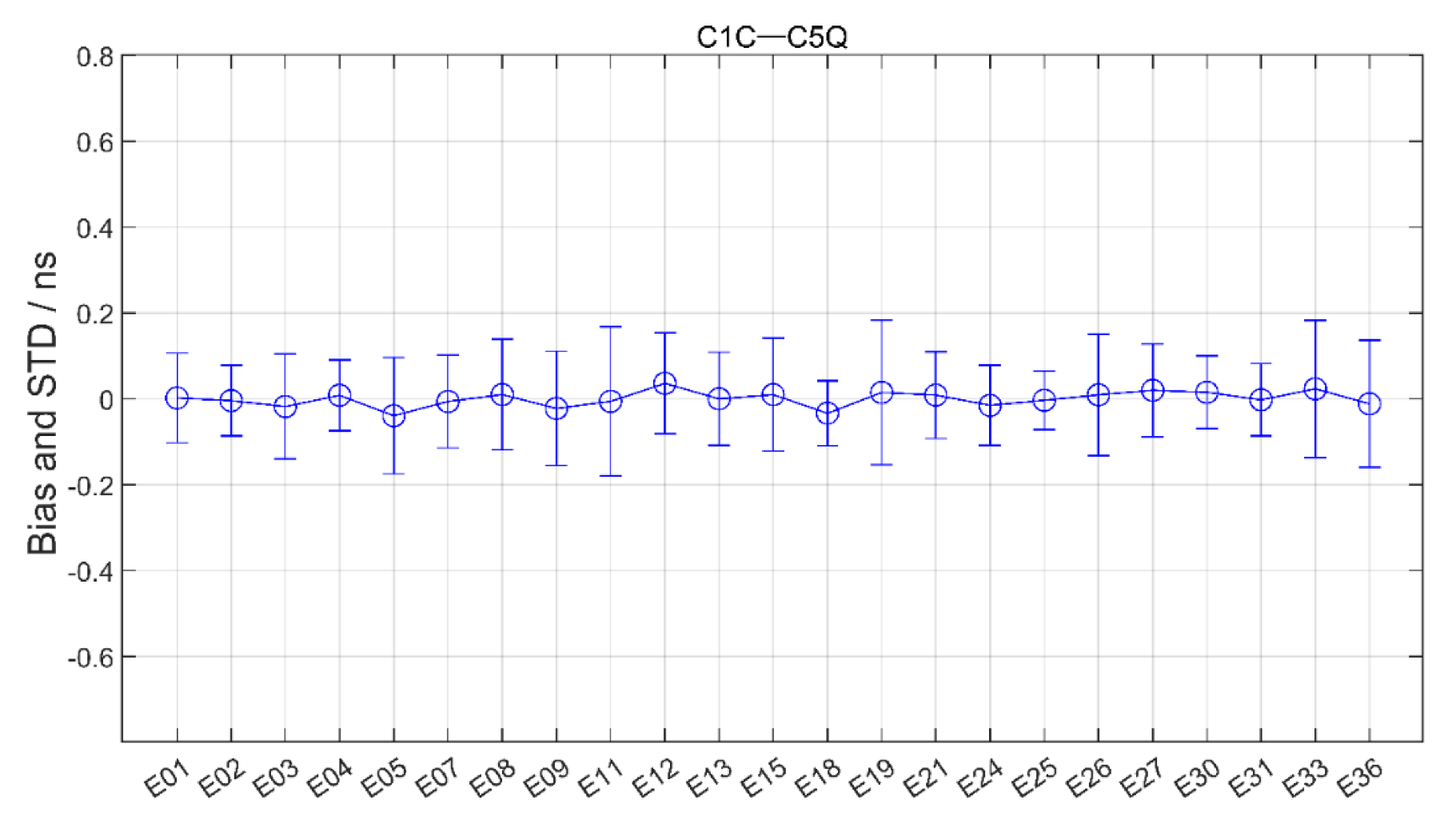
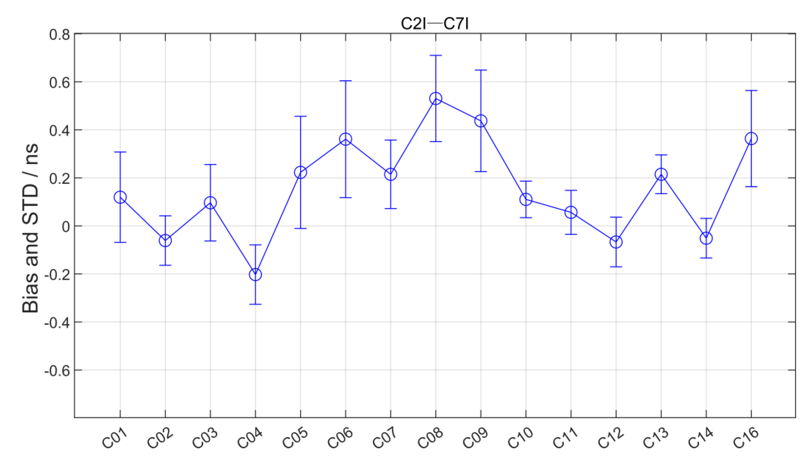
• GPS, GLONASS, Galileo, BDS MEO and IGSO satellite DCB show better stability, while the BDS GEO satellite has low stability due to poor data quality. Comparing the estimated satellite DCB with other institutions, the DCB estimated in this manuscript has good consistency. The average biases of the four systems are basically within 0.25 ns, 0.25 ns, 0.2 ns and 0.42 ns, and the STD is basically within 0.25 ns. The consistency of DCB of the BDS-3 satellite is better than that of the BDS-2 satellite. Other DCB types of these systems show stability and consistency with other institutions.

References

1. Haddad, R.; Kovach, K.; Slattery, R. GPS modernization and beyond/2020 IEEE/ION Position, Location and Navigation Symposium (PLANS). IEEE 2020, 399–406. Available online: https://ieeexplore.ieee.org/abstract/document/9110167 (accessed on 12 October 2022).
2. Thomas, M.L. Evolution of GPS systems architecture and its impacts. Commun. IIMA 2010, 10, 3. [Google Scholar]
3. Fontana, R.; Latterman, D. GPS Modernization and the Future. In Proceedings of the IAIN World Congress and the 56th Annual Meeting of The Institute of Navigation (2000), San Diego, CA, USA, 26–28 June 2000; pp. 222–231. [Google Scholar]
4. Thoelert, S.; Steigenberger, P.; Montenbruck, O. Signal analysis of the first GPS III satellite. GPS Solut. 2019, 23, 92. [Google Scholar] [CrossRef]
5. Paziewski, J. Recent advances and perspectives for positioning and applications with smartphone GNSS observations. Meas. Sci. Technol. 2020, 31, 091001. [Google Scholar] [CrossRef]
6. Priyanka, C.; Ratnam, D.V.; Sai, K.S.G. A Review on design of low noise amplifiers for global navigational satellite system. AIMS Electron. Electr. Eng. 2021, 5, 206–229. [Google Scholar] [CrossRef]
7. Julien, O.; Priya, L.; Issler, J.L. Estimating the ionospheric delay using GPS/Galileo signals in the E5 band. Inside GNSS 2015, 10, 55–64. [Google Scholar]
8. Li, M.; Yuan, Y. Estimation and Analysis of BDS2 and BDS3 Differential Code Biases and Global Ionospheric Maps Using BDS Observations. Remote Sens 2021, 13, 370. [Google Scholar] [CrossRef]
9. Yang, Y.; Liu, L.; Li, J.; Yang, Y.; Zhang, T.; Mao, Y.; Sun, B.; Ren, X. Featured services and performance of BDS-3. Sci. Bull. 2021, 66, 2135–2143. [Google Scholar] [CrossRef]
10. Jin, S.; Park, J.U.; Wang, J.L. Electron density profiles derived from ground-based GPS observations. J. Navig. 2006, 59, 395–401. [Google Scholar] [CrossRef] [Green Version]
11. Isioye, O.A.; Combrinck, L.; Botai, J.O.; Munghemezulu, C. The potential for observing African weather with GNSS remote sensing. Adv. Meteorol. 2015, 2015, 723071. [Google Scholar] [CrossRef] [Green Version]
12. Hegarty, C.J.; Chatre, E. Evolution of the global navigation satellite system (gnss). Proc. IEEE 2008, 96, 1902–1917. [Google Scholar] [CrossRef]
13. Wang, H.; Hou, Y.; Dang, Y.; Bei, J.; Zhang, Y.; Wang, J.; Cheng, Y.; Gu, S. Long-term time-varying characteristics of UPD products generated by a global and regional network and their interoperable application in PPP. Adv. Space Res. 2021, 67, 883–901. [Google Scholar] [CrossRef]
14. Wang, H.; Dang, Y.; Hou, Y.; Bei, J.; Wang, J.; Bai, G.; Cheng, Y.; Zhang, S. Rapid and precise solution of the whole network of thousands of stations in China based on PPP network solution by UPD fixed technology. Acta Geod. Cart. 2020, 49, 278–291. [Google Scholar]
15. Ma, H.; Zhao, Q.; Verhagen, S. Assessing the performance of multi-GNSS PPP-RTK in the local area. Remote Sens. 2020, 12, 3343. [Google Scholar] [CrossRef]
16. Shen, N.; Chen, L.; Lu, X. Interactive multiple-model vertical vibration detection of structures based on high-frequency GNSS observations. GPS Solut. 2022, 26, 1–19. [Google Scholar] [CrossRef]
17. Shen, N.; Chen, L.; Chen, R. Displacement detection based on Bayesian inference from GNSS kinematic positioning for deformation monitoring. Mech. Syst. Signal. Pract. 2022, 167, 108570. [Google Scholar] [CrossRef]
18. Xu, X.; Li, M.; Li, W.; Liu, J. Performance Analysis of Beidou-2/Beidou-3e Combined Solution with Emphasis on Precise Orbit Determination and Precise Point Positioning. Sensors 2018, 18, 135. [Google Scholar] [CrossRef] [Green Version]
19. Xu, X.; Wang, X.; Liu, J.; Zhao, Q. Characteristics of BD3 Global Service Satellites: POD, Open Service Signal and Atomic Clock Performance. Remote Sens. 2019, 11, 1559. [Google Scholar] [CrossRef] [Green Version]
20. Ma, H.; Psychas, D.; Xing, X. Influence of the inhomogeneous troposphere on GNSS positioning and integer ambiguity resolution. Adv. Space Res. 2021, 67, 1914–1928. [Google Scholar] [CrossRef]
21. Ma, H.; Verhagen, S. Precise point positioning on the reliable detection of tropospheric model errors. Sensors 2020, 20, 1634. [Google Scholar] [CrossRef] [Green Version]
22. Psychas, D.; Bruno, J.; Massarweh, L. Towards sub-meter positioning using Android raw GNSS measurements. In Proceedings of the 32nd International Technical Meeting of the Satellite Division of The Institute of Navigation (ION GNSS+ 2019), Miami, FL, USA, 16–20 September 2019; pp. 3917–3931. [Google Scholar]
23. Ma, H.; Verhagen, S.; Psychas, D.; Monico, J.F.G.; Marques, H.A. Flight-test evaluation of integer ambiguity resolution enabled PPP. J. Surv. Eng. 2021, 147, 04021013. [Google Scholar] [CrossRef]
24. Seok, H.W.; Ansari, K.; Panachai, C. Individual performance of multi-GNSS signals in the determination of STEC over Thailand with the applicability of Klobuchar model. Adv. Space Res. 2022, 69, 1301–1318. [Google Scholar] [CrossRef]
25. Wilson, B.D.; Mannucci, A.J. Instrumental biases in ionospheric measurements derived from GPS data. In Proceedings of the ION GPS 1993 (Institute of Navigation), Salt Lake City, UT, USA, 22–24 September 1993; pp. 1343–1351. [Google Scholar]
26. Davis, J.L.; Cosmo, M.L.; Elgered, G. Using the Global Positioning System to study the atmosphere of the Earth: Overview and prospects. GPS Trends Precise Terr. Airborne Spaceborne Appl. 1996, 233–242. Available online: https://linkspringer.53yu.com/chapter/10.1007/978-3-642-80133-4_37 (accessed on 12 October 2022).
27. Komjathy, A.; Yang, Y.M.; Meng, X. Review and perspectives: Understanding natural-hazards-generated ionospheric perturbations using GPS measurements and coupled modeling. Radio Sci. 2016, 51, 951–961. [Google Scholar] [CrossRef]
28. Panda, S.K.; Haralambous, H.; Moses, M. Ionospheric and plasmaspheric electron contents from space-time collocated digisonde, COSMIC, and GPS observations and model assessments. Acta Astronaut. 2021, 179, 619–635. [Google Scholar] [CrossRef]
29. Marković, M. Determination of total electron content in the ionosphere using GPS technology. Geonauka 2014, 2, 1–9. [Google Scholar] [CrossRef] [Green Version]
30. Wang, H.; Wang, C.; Wang, J.X. Global characteristics of the second-order ionospheric delay error using inversion of electron density profiles from COSMIC occultation data. Sci. China Phys. Mech. 2014, 57, 365–374. [Google Scholar] [CrossRef]
31. Brunini, C.; Azpilicueta, F. GPS slant total electron content accuracy using the single layer model under different geomagnetic regions and ionospheric conditions. J. Geod. 2010, 84, 293–304. [Google Scholar] [CrossRef]
32. Wang, X.L.; Wan, Q.T.; Ma, G.Y. The influence of ionospheric thin shell height on TEC retrieval from GPS observation. Res. Astron. Astrophys. 2016, 16, 016. [Google Scholar] [CrossRef] [Green Version]
33. Liu, J.; Wang, Z.; Zhang, H. Comparison and Consistency Research of Regional Ionospheric TEC Models Based on GPS Measurements. Geomat. Inf. Ence Wuhan Univ. 2008, 33, 479–483. [Google Scholar]
34. Zhang, H.; Han, W.; Huang, L. Modeling global ionospheric delay with IGS ground-based GNSS observations. Geomat. Inf. Sci. Wuhan Univ. 2012, 37, 1186–1189. [Google Scholar]
35. Shagimuratov, I.I.; Chernyak, Y.V.; Zakharenkova, I.E. Use of GLONASS for studying the ionosphere. Russ. J. Phys. Chem. B+ 2015, 9, 770–777. [Google Scholar] [CrossRef]
36. Yasyukevich, Y.V.; Mylnikova, A.A.; Polyakova, A.S. Estimating the total electron content absolute value from the GPS/GLONASS data. Results Phys. 2015, 5, 32–33. [Google Scholar] [CrossRef] [Green Version]
37. Zhang, X.; Xie, W.; Ren, X. Influence of the GLONASS inter-frequency bias on differential code bias estimation and ionospheric modeling. GPS Solut. 2017, 21, 1355–1367. [Google Scholar] [CrossRef]
38. Xue, J.; Song, S.; Liao, X. Estimating and assessing Galileo navigation system satellite and receiver differential code biases using the ionospheric parameter and differential code bias joint estimation approach with multi-GNSS observations. Radio Sci. 2016, 51, 271–283. [Google Scholar] [CrossRef] [Green Version]
39. Bidaine, B.; Warnant, R. Ionosphere modeling for Galileo single frequency users: Illustration of the combination of the NeQuick model and GNSS data ingestion. Adv. Space Res. 2011, 47, 312–322. [Google Scholar] [CrossRef] [Green Version]
40. Hernández-Pajares, M.; Lyu, H.; Garcia-Fernandez, M. A new way of improving global ionospheric maps by ionospheric tomography: Consistent combination of multi-GNSS and multi-space geodetic dual-frequency measurements gathered from vessel-, LEO-and ground-based receivers. J. Geod. 2020, 94, 1–16. [Google Scholar] [CrossRef]
41. Zhang, M. Establishment of European Regional Ionosphere Model Based on Spherical Harmonic Functions. J. World Archit. 2021, 5, 5–9. [Google Scholar] [CrossRef]
42. Le, A.Q. Impact of Galileo on global ionosphere map estimation. J. Navig. 2006, 59, 281–292. [Google Scholar] [CrossRef] [Green Version]
43. Li, M.; Zhang, B.; Yuan, Y. Single-frequency precise point positioning (PPP) for retrieving ionospheric TEC from BDS B1 data. GPS Solut 2019, 23, 1–11. [Google Scholar] [CrossRef]
44. Ren, X.; Chen, J.; Li, X. Multi-GNSS contributions to differential code biases determination and regional ionospheric modeling in China. Adv. Space Res. 2020, 65, 221–234. [Google Scholar] [CrossRef]
45. Ren, X.; Zhang, X.; Xie, W. Global ionospheric modeling using multi-GNSS: BeiDou, Galileo, GLONASS and GPS. Sci. Rep. 2016, 6, 33499. [Google Scholar] [CrossRef] [PubMed] [Green Version]
46. Jin, R.; Jin, S.; Feng, G. M_DCB: Matlab code for estimating GNSS satellite and receiver differential code biases. GPS Solut. 2012, 16, 541–548. [Google Scholar] [CrossRef]
47. Dach, R.; Lutz, S.; Walser, P.; Fridez, P. (Eds.) Bernese GNSS Software Version 5.2. User Manual, Astronomical Institute; University of Bern, Bern Open Publishing: Bern, Switzerland, 2015; ISBN 978-3-906813-05-9. [Google Scholar] [CrossRef]
48. Zhang, Q.; Chen, Z.; Yang, Z. A Refined Metric for Multi-GNSS Constellation Availability Assessment in Polar Regions. Adv. Space Res. 2020, 4, 33. [Google Scholar] [CrossRef]
Figure 1. GPS, GLONASS, GALILEO and BDS stations distribution.
Remotesensing 14 05479 g001
Figure 2. Amplitude of solar and geomagnetic activity.
Remotesensing 14 05479 g002
Figure 3. IPPs distribution of (a) GPS, (b) GLONASS, (c) Galileo and (d) BDS.
Remotesensing 14 05479 g003
Figure 4. IPPs trajectory distribution of BDS different orbital satellites.
Remotesensing 14 05479 g004
Figure 5. Biases between different results and CODE GIM at UT 0:00 DOY 213 in 2021: (a) GPS; (b) GLONASS; (c) Galileo; (d) BDS; (e) BDS (MEO + IGSO).
Remotesensing 14 05479 g005
Figure 6. Biases between GIMs and CODE GIMs of four systems during ionospheric quiet days.
Remotesensing 14 05479 g006
Figure 7. Biases between different results and CODE GIM at UT 0:00 DOY 308 in 2021: (a) GPS; (b) GLONASS; (c) Galileo; (d) BDS; (e) BDS (MEO + IGSO).
Remotesensing 14 05479 g007
Figure 8. Biases between GIMs and CODE GIMs of four systems during active ionospheric days.
Remotesensing 14 05479 g008
Figure 9. Region distribution of 0-value (blue region) of four systems at UT 0:00, DOY 213, 2021. (a) GPS; (b) GLONASS; (c) Galileo; (d) BDS; (e) BDS (MEO + IGSO).
Remotesensing 14 05479 g009
Figure 10. Region distribution of 0-value (blue region) of four systems at UT 0:00, DOY 308, 2021. (a) GPS; (b) GLONASS; (c) Galileo; (d) BDS; (e) BDS (MEO + IGSO).
Remotesensing 14 05479 g010
Figure 11. DCB time series of GPS satellites at different ionospheric conditions.
Remotesensing 14 05479 g011
Figure 12. DCB time series of GLONASS satellite at different ionospheric conditions.
Remotesensing 14 05479 g012
Figure 13. Comparison results between DCB and CODE products of GPS satellite.
Remotesensing 14 05479 g013
Figure 14. Comparison results between DCB and CODE products of GLONASS satellite.
Remotesensing 14 05479 g014
Figure 15. DCB time series of Galileo satellite at different ionospheric conditions.
Remotesensing 14 05479 g015
Figure 16. Comparison results between DCB and CAS products of Galileo satellites.
Remotesensing 14 05479 g016
Figure 17. DCB time series of BDS satellites in different ionospheric conditions. (a) is BDS (MEO + IGSO) satellites and (b) is BDS GEO satellites.
Remotesensing 14 05479 g017
Figure 18. Comparison results between DCB and CAS products of BDS satellite.
Remotesensing 14 05479 g018
Figure 19. C1C–C2W DCB time series of GPS satellites.
Remotesensing 14 05479 g019
Figure 20. Comparison results between DCB and CAS products of GPS satellite.
Remotesensing 14 05479 g020
Figure 21. C1C–C2P DCB time series of GLONASS satellites.
Remotesensing 14 05479 g021
Figure 22. Comparison results between DCB and CAS products of GLONASS satellite.
Remotesensing 14 05479 g022
Figure 23. C1C–C5Q DCB time series of Galileo satellites.
Remotesensing 14 05479 g023
Figure 24. Comparison results between DCB and CAS products of Galileo satellite.
Remotesensing 14 05479 g024
Figure 25. C2I–C7I DCB time series of BDS satellites.
Remotesensing 14 05479 g025
Figure 26. Comparison results between DCB and CAS products of BDS satellite.
Remotesensing 14 05479 g026