Abstract
Forests are the largest terrestrial ecosystem carbon pool and provide the most important nature-based climate mitigation pathway. Compared with belowground biomass (BGB) and soil carbon, aboveground biomass (AGB) is more sensitive to human disturbance and climate change. Therefore, accurate forest AGB mapping will help us better assess the mitigation potential of forests against climate change. Here, we developed six models to estimate national forest AGB using six machine learning algorithms based on 52,415 spaceborne Light Detection and Ranging (LiDAR) footprints and 22 environmental features for China in 2007. The results showed that the ensemble model generated by the stacking algorithm performed best with a determination coefficient (R2) of 0.76 and a root mean square error (RMSE) of 22.40 Mg/ha. The verifications at pixel level (R2 = 0.78, RMSE = 16.08 Mg/ha) and provincial level (R2 = 0.53, RMSE = 14.05 Mg/ha) indicated the accuracy of the estimated forest AGB map is satisfactory. The forest AGB density of China was estimated to be 53.16 ± 1.63 Mg/ha, with a total of 11.00 ± 0.34 Pg. Net primary productivity (NPP), normalized difference vegetation index (NDVI), enhanced vegetation index (EVI), average annual rainfall, and annual temperature anomaly are the five most important environmental factors for forest AGB estimation. The forest AGB map we produced is expected to reduce the uncertainty of forest carbon source and sink estimations.
1. Introduction
Forests are the largest carbon pool in terrestrial ecosystems, providing up to 70–90% of terrestrial ecosystem carbon stocks with 31% of the global land area [1,2]. Forests fix carbon by absorbing atmospheric CO2 through photosynthesis to form biomass and soil organic carbon, namely forest carbon sink. The global carbon sink potential of forests amounts to −4 Pg C/year, which can offset about 25% of anthropogenic carbon emissions [3,4]. Meanwhile, forest management pathways such as afforestation and avoiding deforestation provide two thirds of the mitigation potential of cost-effective natural climate solutions under the 2 °C global warming target [5]. When forests are disturbed, the carbons sequestered in forests are released back into the atmosphere in the form of CO2, namely forest carbon source. Tropical forest carbon loss doubled from 0.97 Pg C/year in 2001–2005 to 1.99 Pg C/year in 2015–2019, mainly due to forest conversion (deforestation or conversion of forests to other lands) [6]. Forest aboveground biomass (AGB) is more sensitive to possible anthropogenic disturbance [6] and future climate change [7] than belowground biomass (BGB) and soil carbon. Accurate assessment of forest AGB will help us better understand the spatiotemporal dynamics of forest carbon source and sink in the context of future global change, and clarify the mitigation potential of forests on climate change [8].
The combination of ground-based measurements and remote sensing technology provides a more elegant manner to estimate large scale forest AGB compared with traditional ways [9]. Environmental remote sensing features such as single-band reflectance, vegetation indices, and leaf area index can be provided by optical remote sensing (e.g., the Moderate Resolution Imaging Spectroradiometer, MODIS), then large scale forest AGB estimations are allowed to implement by extrapolating the statistical relationship between in situ AGB and remote sensing features [10]. For example, Piao [11] estimated Chinese forest biomass through establishing an empirical statistical model based on ground measured data and optical remote sensing features. However, optical remote sensing lacks key forest vertical structure parameters (e.g., tree height), resulting in underutilization of forest 3D information in AGB estimation [12]. Active remote sensing such as Light Detection and Ranging (LiDAR) is able to measure more accurate forest 3D parameters to estimate carbon due to its strong penetrability [13]. As an example, Asner et al. [14] retrieved the forest carbon stocks by converting the canopy height derived from the airborne LiDAR data into carbon density using an allometric model for small areas. Large scale ground measurement is the mission objective of spaceborne LiDAR; nevertheless, currently in-orbit satellites (e.g., the Ice, Cloud, and Land Elevation Satellite, ICESat) only provide discrete point data, which needs to be combined with other remote sensing data to perform wall-to-wall mapping [15,16]. For instance, Saatchi et al. [17] produced a benchmark map of tropical forest carbon stocks based on a variety of data included ground measured data, optical imagery, microwave satellite, LiDAR, and other data. Imaging radar is also able to estimate the forest biomass as an active remote sensing technology [12], the problem of information saturation is the bottleneck [18]. Different remote sensing technologies have different advantages and disadvantages, the fusion of multi-source data to compensate the defects of single source data is a ponderable research interest [19].
Machine learning is the cornerstone of artificial intelligence, which is an interdisciplinary subject involving probability theory, statistics, linear algebra, higher mathematics, algorithm complexity theory, and other fields [20]. Relying on the powerful performance of modern computers, machine learning algorithms can simulate human learning behavior, mine useful rules and knowledge from a large number of data information, and constantly reorganize the knowledge structure to achieve the purpose of self-improvement in multiple iterations [21]. Therefore, compared with traditional algorithms, the main advantage of machine learning algorithms is that they can significantly improve the simulation accuracy of phenomena and processes [22]. However, machine learning algorithms also have some thorny shortcomings, such as overfitting and bias problems [23]. Machine learning can be divided into supervised learning, unsupervised learning, and reinforcement learning according to the difference of experience and learning method [20]. Since supervised learning mainly deals with classification and regression problems, it is frequently used in the field of remote sensing by many scholars [24,25].
Forest AGB estimation is essentially a regression problem which can be handled by supervised learning; in this situation, some supervised learning algorithms (e.g., k-Nearest Neighbor, KNN; Random Forest, RF) have been successfully used to construct forest AGB retrieval models [26]. However, there are many other algorithms in the machine learning field, such as gradient boosting (GB) [27], extreme gradient boosting (XGB) [28], light gradient boosting machine (LGBM) [29], and categorical boosting (CatBoost) [30]. Although some of these algorithms have achieved good performance in the regional scale biomass retrieval [31,32], the above-mentioned four algorithms have not been fully explored in the national scale forest AGB mapping [19,33]. Moreover, the performance of single machine learning algorithm is also limited [34]; ensemble algorithms such as stacking [35] can theoretically combine the advantages of multiple algorithms to optimize model performance, thus they have the remarkable potential to improve the reliability of forest AGB estimations [36].
After decades of continuous implementation of forest managements [37], China has become the country with the largest plantation area and the fifth largest forest area in the world [1], which is an excellent testing ground for forest AGB estimation. Hence, the contents of this study are as follows: (1) Based on ground inventory data, spaceborne LiDAR, optical imageries, and climate and topographic data, we developed six forest AGB estimation models using six machine learning algorithms, and assessed the contribution of the environmental features, (2) the AGB values estimated by the six models were verified using an independent ground measured dataset and the Chinese Forest Resources Report (FRR), and (3) the spatially continuous forest AGB map of China was produced using the optimal model, and was compared with the existing products.
2. Materials and Methods
We used six machine learning algorithms to estimate the AGB and adopted a three-stage strategy in the modeling process. In the first stage, allometric statistical relationships were established between the tree heights and AGB measured in the field plots, allowing tree height to be converted into AGB. In the second stage, the forest canopy heights in the ICESat/GLAS footprints were calculated, and these heights were converted into AGB (namely, GLAS-derived AGB) using the allometric models developed in the first stage. In this stage, we extended the AGB values from plot level to GLAS footprint level. In the third stage, machine learning algorithms were used to model the relationship between the environmental features and the GLAS-derived AGB to realize the spatial extrapolation, thereby expanding the GLAS footprint level AGB into wall-to-wall AGB. The follow-up is organized as follows: Section 2.1 describes the forest plot survey data and the allometric relationship results. Section 2.2 describes the ICESat/GLAS data processing process and the data sources of the environmental features. Section 2.3 describes the modeling process of the machine learning algorithms. Section 2.4 describes the verification procedure for the estimated AGB values.
2.1. Forest Inventory Data and Allometric Equation
We collected 1607 forest plot records from a published dataset across China, mainly measured by clear-cutting or harvesting between 2000 and 2008 [38]. The dataset contains AGB, BGB, and dead biomass, as well as geographical coordinates, diameters at breast-height (DBH), and tree heights. We identified the forest type of each record using a forest cover map from a land cover product [39]. Then, records without tree height, AGB, and forest type were filtered out, and 370 records were retained to construct allometric model.
Generally, allometric relationships vary with tree species and climatic conditions, and have spatial heterogeneity. Therefore, considering the number and distribution of samples and possible outliers, we used a power-law function based on bi-square weights robust least squares to fit the relationships between the tree heights and the AGB for two forest types (broadleaf and conifer, derived from the forest cover map) in two climatic geographic regions (N and S, derived from climate zone) [40,41] separately (Figure 1). We evaluated the equations by cross-validation; consequently, tree height explained 65% to 88% of the variation in forest AGB, of which the region N conifer model and the region S broadleaf model were the two with the best performance, while the accuracy of region S conifer model was the lowest (Table 1).
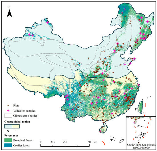
Figure 1.
Spatial distribution of the forest plots in different geographical regions. N denotes north China; S denotes south China. Validation samples are used for validation at the pixel level described in Section 2.4. The land cover product provides three main forest types including broadleaf, conifer, and mixed forest. There are four subtypes in broadleaf, four subtypes in conifer, and two subtypes in mixed forest. Take broadleaf as an example, there are open evergreen broadleaf, closed evergreen broadleaf, open deciduous broadleaf, and closed deciduous broadleaf. The four subtypes were merged to establish allometric relationships for broadleaf in order to have sufficient samples to maintain statistical significance of the results due to the limited number of forest plots, and conifer was treated in the same way. In addition, there were almost no mixed forest samples due to too few pixels of mixed forest, thus we merged the mixed forest pixel to the nearest pixel of other forest types.

Table 1.
Allometric model parameters of different forest types in different geographical regions. AGB = a·Hb, where AGB is the plot aboveground biomass (Mg/ha), H is the mean height of dominant trees from the emergent layer and the canopy layer in a field plot. a and b are the power-law function parameters.
2.2. Remote Sensing Data Collection
2.2.1. Spaceborne LiDAR
We employed the GLAH05 and GLAH14 data from the Geoscience Laser Altimeter System (GLAS) on board the Ice, Cloud, and Land Elevation Satellite (ICESat) for 2005–2009 to extract and filter the forest maximum canopy height (RH100) at the GLAS footprint level using the method described in detail in the previous study [42], and further refined the results using a forest canopy height product [43]. Due to the root mean square error (RMSE) of the product is 4.4 m, the GLAS-derived canopy heights with an absolute difference of 2.2 m or less from the product were regarded as high-confidence data. Finally, 52,415 GLAS footprints were remained, and the forest maximum canopy heights in these footprints were converted to AGB (namely GLAS-derived AGB) through the allometric relationships developed in Section 2.1.
2.2.2. MODIS Dataset
The Moderate Resolution Imaging Spectroradiometer (MODIS) is an important space remote sensing instrument developed by the National Aeronautics and Space Administration (NASA) for Earth observation; it has been providing a large amount of highly accurate scientific datasets for about 20 years. The average and maximum normalized difference vegetation index (NDVI) and enhanced vegetation index (EVI) were calculated through average and maximum composition from MODIS-terra MOD13Q1 data in 2007 using the Google Earth Engine (GEE) on the basis of these two indices are frequently present in the process of establishing forest AGB estimation model [17,44]. The average and maximum leaf area index (LAI), fraction of photosynthetically active radiation (FPAR), and evapotranspiration (ET) were also derived from MOD15A2H and MOD16A2 to represent vegetation canopy structure and energy exchange rate.
2.2.3. NPP and Climate Factors
The amount of carbon required for plant growth is the carbon gain during photosynthesis minus the loss of autotrophic respiration, that is, the net primary productivity (NPP) [45], and the previous study [46] suggests NPP is more closely related to vegetation growth and biomass. Otherwise, the relationship between photosynthesis and plant growth is strongly influenced by climate [47]. Thus, we employed the Global Land Surface Satellite (GLASS) NPP product to stand for vegetation growth of the year 2007 [48]. The average temperature, maximum temperature, minimum temperature, temperature range, total accumulated temperature, average precipitation, and total precipitation for 1978–2007 were calculated from published climate datasets [49] which are downscaled from the CRU TS V4.02 to represent the 30-year mean climate state, and the anomalies of the average precipitation and average temperature in 2007 from the mean climate state were also obtained.
2.2.4. Topography
The Shuttle Radar Topography Mission (SRTM) digital elevation data were measured primarily by the National Aeronautics and Space Administration (NASA) and the National Imagery and Mapping Agency (NIMA). The data cover more than 80% of the global land surface from 56°S to 60°N with the spatial resolution of 1 arc-second (approximately 30 m) [50]. We extracted the surfaces of elevation and slope as terrain variables from SRTM V3 product in the GEE.
2.3. Forest AGB Estimation and Uncertainty Determination
2.3.1. Model Design
A pre-test scheme was employed to filtrate algorithms and environmental features. We first collected ten machine learning algorithms that have been widely used in forest AGB estimation research (Table 2) to conduct a 10-fold cross-validation pre-model on GLAS-derived AGB and 22 environmental features (Table 3) under default parameter, then screened algorithms by model performance which was assessed using the coefficient of determination (R2) and RMSE, and screened environmental features by feature importance which was assessed using the percentage increase in the mean-squared error. Finally, 5 algorithms and 20 environmental factors were retained to establish the forest AGB estimation model (Table 2 and Table 4). Note that in Table 4, using TMP_total_30a as an example, its permutation importance in the XGB model is 0% but 1.62% in the CatBoost model; if it was eliminated, the performance of the XGB did not increase or decrease, whereas the performance of the CatBoost showed an unacceptable decrease, which would affect the fairness of model performance evaluation. Therefore, the environmental features we retained were the union rather than the intersection of features whose permutation importance was more than 1% in Table 4.
Table 2.
Performance of the ten models in the pre-test. * denotes that the model was eliminated due to the low R2 and high RMSE.
Table 3.
Abbreviations and source of the 22 features.
Table 4.
Permutation importance of the 22 features in the pre-test. * denotes that the feature was eliminated due to its importance was less than 1% in all the reserved models.
A single machine learning algorithm may have high fitting accuracy but poor extrapolation ability. Thus, we used the stacking algorithm to integrate multiple machine learning algorithms to generate the ensemble model, and compared it with the model generated by each single retained algorithm to reveal whether the ensemble model is more robust. In order to argue the influence of different base learners on the model performance and determine the optimal construction, we established five stacked models for different base learner combinations based on the retained five algorithms. We gradually enriched base learners in sort of model performance in the pre-test (Table 2) to get different combinations, a simple linear regression model (Ordinary Least Squares, OLS) was selected as the final estimator in order to prevent the stacked model from overfitting. Moreover, the parameters of the five algorithms were set to default. As a consequence, the model performance reported by stacking the five algorithms were better than the other combinations (Table 5). Hence, these five algorithms would be input together into the stacked model in the subsequent modeling process.
Table 5.
Performance of the five stacked model for the different combinations of base learners.
2.3.2. Forest AGB Estimation
According to the model design, six algorithms (RF, GB, XGB, LGBM, CatBoost, and Stacking) were used to estimate forest AGB based on the GLAS-derived AGB and 20 environmental features. All features were resampled to 1000 m. The optimal parameters (Table 6) of the five algorithms (RF, GB, XGB, LGBM, and CatBoost) were determined respectively by a 5-fold cross-validation grid search to produce five AGB estimation models. Next, as the base learners, the five models were input together into the stacking algorithm and the ordinary least squares linear regression model was selected as the final estimator to aggregate the estimations of all the base learners. The six models (RF, GB, XGB, LGBM, CatBoost, and Stacked) were trained and evaluated using a 10-fold cross-validation. The importance of each feature was also assessed using the percentage increase in the mean-squared error. The optimal model was employed to produce the spatially continuous forest AGB map. We used the forest cover map in Section 2.1 to mask the AGB map and used a tree cover product to rectify the pixel values of the map to narrow the impacts of forest disturbances [42,51,52]. The RF, GB, and Stacking algorithms were implemented using the sklearn package in python. The XGB, LGBM, and CatBoost algorithms were implemented using the xgboost package, lightgbm package, and catboost package in python, respectively.
Table 6.
Parameters of the retained algorithms.
2.3.3. Uncertainty Determination
The uncertainty of the model was determined by the estimated values in cross-validation, and it was calculated as follows at the pixel level [42,53]:
where εprediction is the uncertainty of a pixel (Mg/ha); P is the estimated AGB value; N is the fold number of cross-validation; x1, x2, …, xi are the estimated values in cross-validation; μ is the average of all the estimated values in cross-validation.
2.4. Accuracy Assessment
We used an independent forest plot dataset and the Chinese Forest Resources Report (FRR) to verify the accuracy of the estimated AGB values by the six models at the pixel and provincial level, respectively. Owing to it being hard to find sufficient forest survey records for 2007 across China to validate our estimates, we employed an available independent forest plots dataset that was closest to 2007. The independent dataset included 189 samples which were collected from 2011 to 2016 and covered the main forest areas throughout mainland China [54]. Aiming to minimize the effects of the time inconsistencies, we adopted the method manipulated by predecessors [42] to filter and rectify the samples. Finally, 71 records were reserved for verification at the pixel level (Figure 1). We also extracted the forest standing volume of each province (excluding Hong Kong and Macao) from the FRR issued by the State Forest Administration for 2004–2008, and converted the volumes into AGB through a conversion method [38] for verification at the provincial level.
3. Results
3.1. Model Comparison and Accuracy Verification
The Stacked model (R2 = 0.76, RMSE = 22.40 Mg/ha) outperformed the other models by a significant margin, with the CatBoost (R2 = 0.74, RMSE = 22.99 Mg/ha) in second place and the XGB (R2 = 0.73, RMSE = 23.88 Mg/ha) at the bottom (Figure 2). Additionally, the Stacked had a good ability to estimate AGB for different forest types in different geographical regions (Figure 3), and the estimation accuracy was the highest in the broadleaf forest of region N, followed by the broadleaf forest of region S.
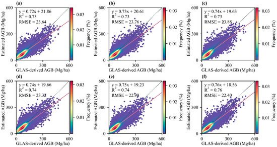
Figure 2.
Performance of the six models in the cross-validation. The dotted lines and red lines are 1:1 line and fitting line, respectively. (a) RF, (b) GB, (c) XGB, (d) LGBM, (e) CatBoost, and (f) Stacked.
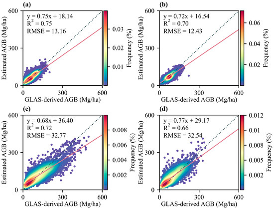
Figure 3.
Performance of the Stacked model in the cross-validation for different forest types in different geographical regions. The dotted lines and red lines are 1:1 line and fitting line, respectively. (a) Broadleaf in region N, (b) conifer in region N, (c) broadleaf in region S, and (d) conifer in region S.
Especially, the verification at the pixel level based on 71 independent samples showed that the accuracy of the AGB values estimated by the Stacked was the best (R2 = 0.78, RMSE = 16.08 Mg/ha), which implies that the model had stronger generalization ability than the others. Simultaneously, the Stacked AGB was closer to the FRR in the verification at the provincial level (R2 = 0.53, RMSE = 14.05 Mg/ha) (Figure 4). Although the estimated AGB was underestimated in 18 provinces and overestimated in 14 provinces, the provincial average AGB density difference between the estimated and the FRR was only 19%. All these indicate that the Stacked model is more capable of estimating the forest AGB. Accordingly, we used the Stacked model to produce the wall-to-wall forest AGB map of China in 2007, and the subsequent analyses were based on the map.
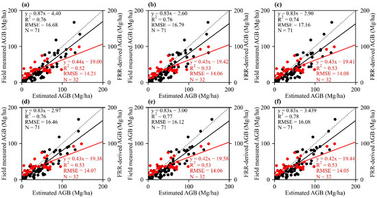
Figure 4.
Validation results of the six models at the pixel and provincial level. The dotted lines are 1:1 line. The black contents are the verifications at the pixel level, and the red contents are the verifications at the provincial level. (a) RF, (b) GB, (c) XGB, (d) LGBM, (e) CatBoost, and (f) Stacked.
3.2. Spatially Continuous Forest AGB Map and Uncertainty Analysis
The spatial distribution of the forest AGB map of China was higher in the region S and lower in the region N, and the high AGB values were primarily distributed in the virgin forests of Nyingchi and Lhoka of Tibet and the Central Range of eastern Taiwan (Figure 5a). Generally, the average forest AGB density of the whole China was 53.16 Mg/ha, with a total of 11.00 Pg. The average AGB density in region N (30.28 Mg/ha) was 44.29% of that in region S. The broadleaf forest contributed 69.26% of the total AGB, which was 2.25 times that of the conifer forest. The spatial distribution of areas with high uncertainty was consistent with that of areas with high AGB (Figure 5b). The uncertainty for the entire study area ranged from 0 to 20.92 Mg/ha, with an average of 1.63 Mg/ha. Since the areas with high AGB were mainly distributed in the broadleaf forest in region S, the average uncertainty in region N (0.60 Mg/ha) was only 26.19% of that in region S, and the uncertainty in broadleaf forest accounted for 66% of that in the entire area of China.
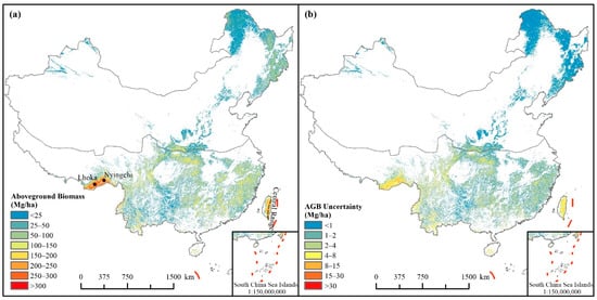
Figure 5.
Spatial distribution of forest AGB and uncertainty in China. (a) Forest AGB and (b) Uncertainty.
3.3. Feature Importance
NPP, NDVI_mean, EVI_mean, PRE_mean_30a, and TMP_2007_30a were the five most important environmental features for forest AGB estimation, while the contributions of Slope and TMP_total_30a were the least (Figure 6). The importance of each environmental feature had a similar distribution pattern in general, whereas there are some differences in detail. For example, the importance of EVI_mean in the RF was obviously lower compared with the others. The importance of TMP_mean_30a in the XGB was significantly higher than that in the others. In the RF, GB, CatBoost, and Stacked, PRE_total_30a was a remarkable feature, but opposite in the XGB and LGBM. Hence, it may be more accurate to measure the impacts of feature on forest AGB estimation by summing up the feature importance results from multiple models.
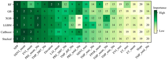
Figure 6.
Feature importance rank of the 20 environmental features in the six models.
4. Discussion
4.1. Comparison and Uncertainties
Forest inventory, remote sensing technology, or ecosystem process simulation are common methods for estimating forest AGB [55]. By setting fixed plots, forest inventory can accurately measure forest biomass at plot scale and provide a precision benchmark for other forest AGB estimation studies [56]. However, forest inventory is time-consuming and labor intensive, which limits its application in large scale forest AGB mapping [9]. Low-cost large-scale forest AGB estimation can be realized based on remote sensing technology by extrapolating the statistical relationship between site scale forest AGB and remote sensing environmental features (such as vegetation index and climate variables) [9,17]. Machine learning is superior to traditional statistical methods, due to it being better at dealing with the nonlinear relationship that may exist between forest AGB and environmental features; thus, it has gradually become the mainstream method for forest AGB estimation [17,42,44,55]. Previous study [57] suggests that the tree model is more suitable for solving ecological remote sensing problems. RF achieves high performance by constructing multiple decision trees and introducing random attribute selection in the training process [57], which may lead to good performance at different scales [58,59,60]. Therefore, although many machine learning algorithms have been adopted by scholars [17,61,62,63], the frequency of RF shows that it has a relatively important position in the current forest AGB estimation. Nevertheless, as the decision tree model is the base model of RF, the shortcomings of decision tree such as overfitting are also reflected in RF. This may be one of the reasons for the greater difference between the Chinese forest AGB estimated by previous studies and FRA data than our result. As we stated in the introduction of this article, the performance of a single model is probably limited [34].
We compared the performance of ten machine learning algorithms in forest AGB estimation in China and highlight that stacking multiple machine learning models can effectively reduce the uncertainty of single machine learning model and increase model stability. Compared with the five best-performing single machine learning algorithms, the accuracy gap between the training and the cross-validation of the Stacked model generated by the stacking algorithm is narrower than the others with the increasing size of the training set according to the learning curves (Figure 7); meanwhile, the Stacked has the highest accuracy in the independent validation (Figure 4), which means the Stacked effectively mitigated overfitting and has stronger generalization ability. In addition, when other sources of uncertainty [17] remain unchanged, we focus on comparing the uncertainty of the six models in the forecasting process (Figure 8). Spatially, the distribution of low uncertainty areas in the Stacked was the broadest, and the high uncertainty areas in the XGB were more than the others. Quantitatively, the average (1.63 Mg/ha) and maximum (20.92 Mg/ha) uncertainty given by the Stacked were the lowest among the six. The total AGB uncertainty of the Stacked was 0.34 Pg, which was 10.53%, 19.05%, 64.95%, 41.38% and 24.44% lower than the RF, GB, XGB, LGBM, and CatBoost, respectively. The results further confirmed that the multi-model fusion method can reduce the uncertainty of forest AGB estimation, which provides more available avenues to improve the accuracy of future carbon estimates.
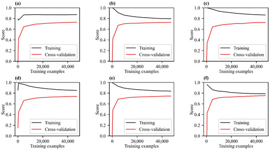
Figure 7.
Learning curves of the six models for different training set sizes. (a) RF, (b) GB, (c) XGB, (d) LGBM, (e) CatBoost, and (f) Stacked.
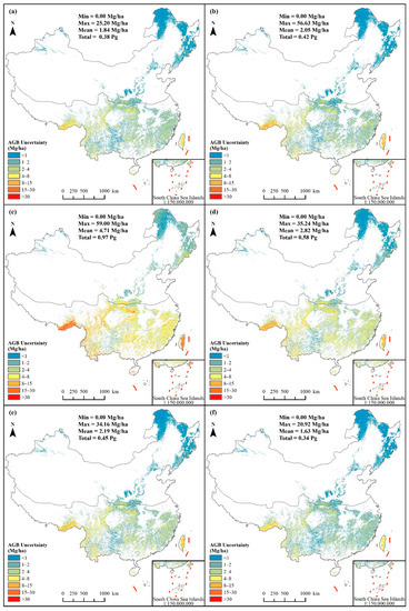
Figure 8.
Spatial distribution of forest AGB uncertainty of the six models. (a) RF; (b) GB; (c) XGB; (d) LGBM; (e) CatBoost; and (f) Stacked.
The density and total of the estimated forest AGB of China in this paper are extremely close to the FRA 2020 [1], with the relative error of −3.57% and −1.61%, respectively (Table 7). It is reasonable for our results to be slightly lower than FRA, on the grounds that the data given by FRA included total living standing tree carbon storage, while only arbor layer AGB was used in our paper and understory vegetation was not included. Compared with the other studies [36,38,49,55] on forest AGB estimation of China using machine learning, our results are in better agreement with FRA. Especially, since we used a larger forest area (219.71 × 10⁴ km2 vs. 164.89 × 10⁴ km2), the AGB density estimated in our paper was lower while the total amount was slightly larger compared with Huang et al., 2019 [36], suggesting that carbon stock estimates are profoundly influenced by different forest cover maps [11,56,64,65]. Although the global forest biomass density estimated by different studies varies greatly, the forest biomass density in China is generally lower compared with the global average in all studies [17,59,66], which indicates Chinese forests are still young and have considerable carbon mitigation potential. Overall, China may need to strengthen the protection and cultivation of forest resources and attach importance to the key role of forest ecosystems in ensuring ecological security and promoting sustainable social development.
Table 7.
Comparison with previous studies.
4.2. Feature Contribution
We highlighted the prominent contribution of NPP and climate factors. To further quantify the impact of NPP and climate factors on forest AGB estimation, we removed them from the modeling features and re-ran the models without changing other parameters. The performances of all the models decreased by about 15% (Table 8), which supported the previous research conclusions [39,40,41,67]. Furthermore, due to inconsistent rules identified from the features in the different models (Figure 6), the persuasiveness of feature importance given by a single model is finite. The true effect of feature on forest AGB during earth system ecological processes may be imprecisely assessed when using the result of only one model. Comprehensive analysis of the feature importance results of multiple models may be able to better define the real contribution of environmental factors on forest AGB estimations.
Table 8.
The accuracy changes of the six models without NPP and climate factors.
4.3. Limitations
The imperfect part of the allometric relationship establishment method is the source of limitations. On the one hand, the relationship between tree height and biomass of different tree species is quite different [67]. However, due to the constraint of the amount of forest plot data, we only established allometric equations for different forest types, which reduces the pertinence of allometric equations and the conversion accuracy from tree height to biomass. On the other hand, we constructed the allometric models using tree height as the unique independent variable, whereas the models are more precise when both tree height and DBH are available [67]. Terrestrial laser scanning (TLS) and unmanned aerial vehicle (UAV) LiDAR are the two main methods for extracting DBH at present; unfortunately, these two modes still present challenges in large-scale DBH parameter measurement [68,69,70]. In conclusion, more available forest plot data and reliable determination of DBH parameters over a wide range are the keys to improving the accuracy of our results.
5. Conclusions
We compared the results of six machine learning models (RF, GB, XGB, LGBM, CatBoost, and Stacked) for forest AGB estimation in China. The performances of the Stacked were the best (R2 = 0.76, RMSE = 22.40 Mg/ha) in the 10-fold cross-validation, and the forest AGB mapped by the Stacked well correlated with the independent forest plot dataset (R2 = 0.78, RMSE = 16.08 Mg/ha) and the FRR (R2 = 0.53, RMSE = 14.05 Mg/ha), respectively. The estimated average forest AGB density of China was 53.16 ± 1.63 Mg/ha, with a total of 11.00 ± 0.34 Pg. Our results were extremely approximate to the FRA at the average level (relative error = −3.57%). In contrast to previous studies, we highlighted the important role of model integration in improving the performance of forest AGB estimation and reducing uncertainty. However, the unavailability of large scale DBH data limits the further improvement of accuracy. In addition, the long time series forest AGB dataset provides basic data for studying the dynamic change of forest carbon source and sink, which is one of the future research interests.
Author Contributions
Conceptualization, Z.G.; data curation, Z.T. and X.X.; formal analysis, Z.T. and X.X.; methodology, Z.T. and X.X.; project administration, Z.G.; supervision, Y.L. and Z.G.; writing—original draft, Z.T., X.X. and Y.H.; writing—review and editing, Z.T., X.X. and Y.H. All authors have read and agreed to the published version of the manuscript.
Funding
This research was supported by the Open Innovation Project of the Technology Innovation Center for Land Spatial Eco-restoration in Metropolitan Area, MNR (grant No. CXZX202206).
Data Availability Statement
The forest inventory dataset was published in [32]. The land cover product was published in [33]. The climate zone data can be obtained from the Resources and Environment Science and Data Center (https://www.resdc.cn/data.aspx?DATAID=243 (accessed on 7 June 2022)). The ICESat/GLAS dataset can be obtained from the National Snow and Ice Data Center (NSIDC; https://nsidc.org/data/icesat (accessed on 7 June 2022)). The MODIS dataset can be obtained from the Earth Observing System Data and Information System (EOSDIS; https://search.earthdata.nasa.gov/search (accessed on 30 August 2022)). The NPP dataset can be obtained from the Global Land Surface Satellite (GLASS) Product suite (http://www.glass.umd.edu/Download.html (accessed on 22 June 2022)). The precipitation and temperature dataset were published in [41]. The topography dataset can be obtained from the US Geological Survey (USGS; https://earthexplorer.usgs.gov (accessed on 13 July 2022)).
Conflicts of Interest
The authors declare no conflict of interest.
References
- FAO. Global Forest Resources Assessment 2020; FAO: Quebec City, QC, Canada, 2020. [Google Scholar]
- Houghton, R.A.; Hall, F.; Goetz, S.J. Importance of biomass in the global carbon cycle. J. Geophys. Res. Biogeosciences 2009, 114, G00E03. [Google Scholar] [CrossRef]
- Houghton, R.A.; Nassikas, A.A. Negative emissions from stopping deforestation and forest degradation, globally. Glob. Chang. Biol. 2018, 24, 350–359. [Google Scholar] [CrossRef] [PubMed]
- Friedlingstein, P.; O’Sullivan, M.; Jones, M.W.; Andrew, R.M.; Hauck, J.; Olsen, A.; Peters, G.P.; Peters, W.; Pongratz, J.; Sitch, S.; et al. Global Carbon Budget 2020. Earth Syst. Sci. Data 2020, 12, 3269–3340. [Google Scholar] [CrossRef]
- Griscom, B.W.; Adams, J.; Ellis, P.W.; Houghton, R.A.; Lomax, G.; Miteva, D.A.; Schlesinger, W.H.; Shoch, D.; Siikamäki, J.V.; Smith, P.; et al. Natural climate solutions. Proc. Natl. Acad. Sci. USA 2017, 114, 11645–11650. [Google Scholar] [CrossRef]
- Feng, Y.; Zeng, Z.; Searchinger, T.D.; Ziegler, A.D.; Wu, J.; Wang, D.; He, X.; Elsen, P.R.; Ciais, P.; Xu, R.; et al. Doubling of annual forest carbon loss over the tropics during the early twenty-first century. Nat. Sustain. 2022, 5, 444–451. [Google Scholar] [CrossRef]
- Gatti, L.V.; Gloor, M.; Miller, J.B.; Doughty, C.E.; Malhi, Y.; Domingues, L.G.; Basso, L.S.; Martinewski, A.; Correia, C.S.C.; Borges, V.F.; et al. Drought sensitivity of Amazonian carbon balance revealed by atmospheric measurements. Nature 2014, 506, 76–80. [Google Scholar] [CrossRef] [PubMed]
- IPCC. 2006 IPCC Guidelines for National Greenhouse Gas Inventories; Institute for Global Environmental Strategies: Hayama, Japan, 2006. [Google Scholar]
- Lu, D.; Chen, Q.; Wang, G.; Liu, L.; Li, G.; Moran, E. A survey of remote sensing-based aboveground biomass estimation methods in forest ecosystems. Int. J. Digit. Earth 2016, 9, 63–105. [Google Scholar] [CrossRef]
- Chirici, G.; Barbati, A.; Corona, P.; Marchetti, M.; Travaglini, D.; Maselli, F.; Bertini, R. Non-parametric and parametric methods using satellite images for estimating growing stock volume in alpine and Mediterranean forest ecosystems. Remote Sens. Environ. 2008, 112, 2686–2700. [Google Scholar] [CrossRef]
- Piao, S. Forest biomass carbon stocks in China over the past 2 decades: Estimation based on integrated inventory and satellite data. J. Geophys. Res. 2005, 110, G01006. [Google Scholar] [CrossRef]
- Patenaude, G.; Milne, R.; Dawson, T.P. Synthesis of remote sensing approaches for forest carbon estimation: Reporting to the Kyoto Protocol. Environ. Sci. Policy 2005, 8, 161–178. [Google Scholar] [CrossRef]
- Lefsky, M.A.; Cohen, W.B.; Parker, G.G.; Harding, D.J. Lidar Remote Sensing for Ecosystem Studies: Lidar, an emerging remote sensing technology that directly measures the three-dimensional distribution of plant canopies, can accurately estimate vegetation structural attributes and should be of particular interest to forest, landscape, and global ecologists. BioScience 2002, 52, 19–30. [Google Scholar] [CrossRef]
- Asner, G.P.; Powell, G.V.N.; Mascaro, J.; Knapp, D.E.; Clark, J.K.; Jacobson, J.; Kennedy-Bowdoin, T.; Balaji, A.; Paez-Acosta, G.; Victoria, E.; et al. High-resolution forest carbon stocks and emissions in the Amazon. Proc. Natl. Acad. Sci. USA 2010, 107, 16738–16742. [Google Scholar] [CrossRef]
- Lefsky, M.A.; Cohen, W.B.; Spies, T.A. An evaluation of alternate remote sensing products for forest inventory, monitoring, and mapping of Douglas-fir forests in western Oregon. Can. J. For. Res. 2001, 31, 78–87. [Google Scholar] [CrossRef]
- Silva, C.A.; Duncanson, L.; Hancock, S.; Neuenschwander, A.; Thomas, N.; Hofton, M.; Fatoyinbo, L.; Simard, M.; Marshak, C.Z.; Armston, J.; et al. Fusing simulated GEDI, ICESat-2 and NISAR data for regional aboveground biomass mapping. Remote Sens. Environ. 2021, 253, 112234. [Google Scholar] [CrossRef]
- Saatchi, S.S.; Harris, N.L.; Brown, S.; Lefsky, M.; Mitchard, E.T.A.; Salas, W.; Zutta, B.R.; Buermann, W.; Lewis, S.L.; Hagen, S.; et al. Benchmark map of forest carbon stocks in tropical regions across three continents. Proc. Natl. Acad. Sci. USA 2011, 108, 9899–9904. [Google Scholar] [CrossRef] [PubMed]
- Santoro, M.; Beer, C.; Cartus, O.; Schmullius, C.; Shvidenko, A.; McCallum, I.; Wegmüller, U.; Wiesmann, A. Retrieval of growing stock volume in boreal forest using hyper-temporal series of Envisat ASAR ScanSAR backscatter measurements. Remote Sens. Environ. 2011, 115, 490–507. [Google Scholar] [CrossRef]
- Abbas, S.; Wong, M.S.; Wu, J.; Shahzad, N.; Muhammad Irteza, S. Approaches of Satellite Remote Sensing for the Assessment of Above-Ground Biomass across Tropical Forests: Pan-tropical to National Scales. Remote Sens. 2020, 12, 3351. [Google Scholar] [CrossRef]
- Jordan, M.I.; Mitchell, T.M. Machine learning: Trends, perspectives, and prospects. Science 2015, 349, 255–260. [Google Scholar] [CrossRef] [PubMed]
- Mitchell, T.M. Machine Learning; McGraw-HillK: New York, NY, USA, 1997; Volume 1. [Google Scholar]
- Sun, S.L.; Cao, Z.H.; Zhu, H.; Zhao, J. A Survey of Optimization Methods from a Machine Learning Perspective. IEEE Trans. Cybern. 2020, 50, 3668–3681. [Google Scholar] [CrossRef] [PubMed]
- Srivastava, N.; Hinton, G.; Krizhevsky, A.; Sutskever, I.; Salakhutdinov, R. Dropout: A Simple Way to Prevent Neural Networks from Overfitting. J. Mach. Learn. Res. 2014, 15, 1929–1958. [Google Scholar]
- Cheng, G.; Han, J.W. A survey on object detection in optical remote sensing images. ISPRS J. Photogramm. Remote Sens. 2016, 117, 11–28. [Google Scholar] [CrossRef]
- Ali, I.; Greifeneder, F.; Stamenkovic, J.; Neumann, M.; Notarnicola, C. Review of Machine Learning Approaches for Biomass and Soil Moisture Retrievals from Remote Sensing Data. Remote Sens. 2015, 7, 16398–16421. [Google Scholar] [CrossRef]
- Rex, F.E.; Silva, C.A.; Dalla Corte, A.P.; Klauberg, C.; Mohan, M.; Cardil, A.; Silva, V.S.d.; Almeida, D.R.A.d.; Garcia, M.; Broadbent, E.N.; et al. Comparison of Statistical Modelling Approaches for Estimating Tropical Forest Aboveground Biomass Stock and Reporting Their Changes in Low-Intensity Logging Areas Using Multi-Temporal LiDAR Data. Remote Sens. 2020, 12, 1498. [Google Scholar] [CrossRef]
- Friedman, J.H. Greedy function approximation: A gradient boosting machine. Ann. Stat. 2001, 29, 1189–1232. [Google Scholar] [CrossRef]
- Chen, T.; Guestrin, C. XGBoost. In Proceedings of the 22nd ACM SIGKDD International Conference on Knowledge Discovery and Data Mining, New York, NY, USA, 13–17 August 2016; pp. 785–794. [Google Scholar]
- Ke, G.; Meng, Q.; Finley, T.; Wang, T.; Chen, W.; Ma, W.; Ye, Q.; Liu, T.-Y. LightGBM: A Highly Efficient Gradient Boosting Decision Tree. In Proceedings of the 31st International Conference on Neural Information Processing Systems, Long Beach, CA, USA, 4–9 December 2017; pp. 3149–3157. [Google Scholar]
- Prokhorenkova, L.; Gusev, G.; Vorobev, A.; Dorogush, A.V.; Gulin, A. CatBoost: Unbiased Boosting with Categorical Features. In Proceedings of the 32nd International Conference on Neural Information Processing Systems, Montreal, QC, Canada, 3–8 December 2018; pp. 6639–6649. [Google Scholar]
- Luo, M.; Wang, Y.; Xie, Y.; Zhou, L.; Qiao, J.; Qiu, S.; Sun, Y. Combination of Feature Selection and CatBoost for Prediction: The First Application to the Estimation of Aboveground Biomass. Forests 2021, 12, 216. [Google Scholar] [CrossRef]
- Li, Y.; Li, M.; Li, C.; Liu, Z. Forest aboveground biomass estimation using Landsat 8 and Sentinel-1A data with machine learning algorithms. Sci. Rep. 2020, 10, 9952. [Google Scholar] [CrossRef]
- Ahmad, A.; Gilani, H.; Ahmad, S.R. Forest Aboveground Biomass Estimation and Mapping through High-Resolution Optical Satellite Imagery—A Literature Review. Forests 2021, 12, 914. [Google Scholar] [CrossRef]
- Mendes-Moreira, J.; Soares, C.; Jorge, A.M.; Sousa, J.F.D. Ensemble approaches for regression. ACM Comput. Surv. 2012, 45, 1–40. [Google Scholar] [CrossRef]
- Wolpert, D.H. Stacked generalization. Neural Netw. 1992, 5, 241–259. [Google Scholar] [CrossRef]
- Zhang, Y.; Ma, J.; Liang, S.; Li, X.; Liu, J. A stacking ensemble algorithm for improving the biases of forest aboveground biomass estimations from multiple remotely sensed datasets. GIScience Remote Sens. 2022, 59, 234–249. [Google Scholar] [CrossRef]
- Chen, C.; Park, T.; Wang, X.; Piao, S.; Xu, B.; Chaturvedi, R.K.; Fuchs, R.; Brovkin, V.; Ciais, P.; Fensholt, R.; et al. China and India lead in greening of the world through land-use management. Nat. Sustain. 2019, 2, 122–129. [Google Scholar] [CrossRef] [PubMed]
- Luo, Y.; Wang, X.; Zhang, X.; Lu, F. Biomass and Its Allocation of Forest Ecosystems in China; Chinese Forestry Publishing House Press: Beijing, China, 2013. [Google Scholar]
- Zhang, X.; Liu, L.; Chen, X.; Gao, Y.; Xie, S.; Mi, J. GLC_FCS30: Global land-cover product with fine classification system at 30 m using time-series Landsat imagery. Earth Syst. Sci. Data 2021, 13, 2753–2776. [Google Scholar] [CrossRef]
- Zhang, J.; Liu, X.; Tan, Z.; Chen, Q. Mapping of the north-south demarcation zone in China based on GIS. J. Lanzhou Univ. Nat. Sci. 2012, 48, 28–33. [Google Scholar]
- Jiang, J.; Jiang, D.; Lin, Y. Monsoon Area and Precipitation over China for 1961–2009. Chin. J. Atmos. Sci. 2015, 39, 722–730. [Google Scholar]
- Huang, H.; Liu, C.; Wang, X.; Zhou, X.; Gong, P. Integration of multi-resource remotely sensed data and allometric models for forest aboveground biomass estimation in China. Remote Sens. Environ. 2019, 221, 225–234. [Google Scholar] [CrossRef]
- Simard, M.; Pinto, N.; Fisher, J.B.; Baccini, A. Mapping forest canopy height globally with spaceborne lidar. J. Geophys. Res. 2011, 116, G04021. [Google Scholar] [CrossRef]
- Su, Y.; Guo, Q.; Xue, B.; Hu, T.; Alvarez, O.; Tao, S.; Fang, J. Spatial distribution of forest aboveground biomass in China: Estimation through combination of spaceborne lidar, optical imagery, and forest inventory data. Remote Sens. Environ. 2016, 173, 187–199. [Google Scholar] [CrossRef]
- Green, J.K.; Keenan, T.F. The limits of forest carbon sequestration. Science 2022, 376, 692–693. [Google Scholar] [CrossRef]
- Richardson, A.D.; Carbone, M.S.; Keenan, T.F.; Czimczik, C.I.; Hollinger, D.Y.; Murakami, P.; Schaberg, P.G.; Xu, X. Seasonal dynamics and age of stemwood nonstructural carbohydrates in temperate forest trees. New Phytol. 2013, 197, 850–861. [Google Scholar] [CrossRef]
- Richardson, A.D.; Anderson, R.S.; Arain, M.A.; Barr, A.G.; Bohrer, G.; Chen, G.; Chen, J.M.; Ciais, P.; Davis, K.J.; Desai, A.R.; et al. Terrestrial biosphere models need better representation of vegetation phenology: Results from the North American Carbon Program Site Synthesis. Glob. Chang. Biol. 2012, 18, 566–584. [Google Scholar] [CrossRef]
- Zheng, Y.; Shen, R.; Wang, Y.; Li, X.; Liu, S.; Liang, S.; Chen, J.M.; Ju, W.; Zhang, L.; Yuan, W. Improved estimate of global gross primary production for reproducing its long-term variation, 1982–2017. Earth Syst. Sci. Data 2020, 12, 2725–2746. [Google Scholar] [CrossRef]
- Peng, S.; Ding, Y.; Liu, W.; Li, Z. 1 km monthly temperature and precipitation dataset for China from 1901 to 2017. Earth Syst. Sci. Data 2019, 11, 1931–1946. [Google Scholar] [CrossRef]
- Farr, T.G.; Rosen, P.A.; Caro, E.; Crippen, R.; Duren, R.; Hensley, S.; Kobrick, M.; Paller, M.; Rodriguez, E.; Roth, L.; et al. The Shuttle Radar Topography Mission. Rev. Geophys. 2007, 45, RG2004. [Google Scholar] [CrossRef]
- Sexton, J.O.; Song, X.-P.; Feng, M.; Noojipady, P.; Anand, A.; Huang, C.; Kim, D.-H.; Collins, K.M.; Channan, S.; DiMiceli, C.; et al. Global, 30-m resolution continuous fields of tree cover: Landsat-based rescaling of MODIS vegetation continuous fields with lidar-based estimates of error. Int. J. Digit. Earth 2013, 6, 427–448. [Google Scholar] [CrossRef]
- Asner, G.P.; Hughes, R.F.; Mascaro, J.; Uowolo, A.L.; Knapp, D.E.; Jacobson, J.; Kennedy-Bowdoin, T.; Clark, J.K. High-resolution carbon mapping on the million-hectare Island of Hawaii. Front. Ecol. Environ. 2011, 9, 434–439. [Google Scholar] [CrossRef]
- Chen, Q.; Vaglio Laurin, G.; Valentini, R. Uncertainty of remotely sensed aboveground biomass over an African tropical forest: Propagating errors from trees to plots to pixels. Remote Sens. Environ. 2015, 160, 134–143. [Google Scholar] [CrossRef]
- Zhu, J.; Hu, H.; Tao, S.; Chi, X.; Li, P.; Jiang, L.; Ji, C.; Zhu, J.; Tang, Z.; Pan, Y.; et al. Carbon stocks and changes of dead organic matter in China’s forests. Nat. Commun. 2017, 8, 151. [Google Scholar] [CrossRef]
- Chang, Z.; Hobeichi, S.; Wang, Y.-P.; Tang, X.; Abramowitz, G.; Chen, Y.; Cao, N.; Yu, M.; Huang, H.; Zhou, G.; et al. New Forest Aboveground Biomass Maps of China Integrating Multiple Datasets. Remote Sens. 2021, 13, 2892. [Google Scholar] [CrossRef]
- Tang, X.; Zhao, X.; Bai, Y.; Tang, Z.; Wang, W.; Zhao, Y.; Wan, H.; Xie, Z.; Shi, X.; Wu, B.; et al. Carbon pools in China’s terrestrial ecosystems: New estimates based on an intensive field survey. Proc. Natl. Acad. Sci. USA 2018, 115, 4021–4026. [Google Scholar] [CrossRef]
- Belgiu, M.; Drăguţ, L. Random forest in remote sensing: A review of applications and future directions. ISPRS J. Photogramm. Remote Sens. 2016, 114, 24–31. [Google Scholar] [CrossRef]
- Ghosh, S.M.; Behera, M.D. Aboveground biomass estimation using multi-sensor data synergy and machine learning algorithms in a dense tropical forest. Appl. Geogr. 2018, 96, 29–40. [Google Scholar] [CrossRef]
- Hu, T.; Su, Y.; Xue, B.; Liu, J.; Zhao, X.; Fang, J.; Guo, Q. Mapping Global Forest Aboveground Biomass with Spaceborne LiDAR, Optical Imagery, and Forest Inventory Data. Remote Sens. 2016, 8, 565. [Google Scholar] [CrossRef]
- Chi, H.; Sun, G.; Huang, J.; Guo, Z.; Ni, W.; Fu, A. National Forest Aboveground Biomass Mapping from ICESat/GLAS Data and MODIS Imagery in China. Remote Sens. 2015, 7, 5534–5564. [Google Scholar] [CrossRef]
- Beaudoin, A.; Bernier, P.Y.; Guindon, L.; Villemaire, P.; Guo, X.J.; Stinson, G.; Bergeron, T.; Magnussen, S.; Hall, R.J. Mapping attributes of Canada’s forests at moderate resolution through kNN and MODIS imagery. Can. J. For. Res. 2014, 44, 521–532. [Google Scholar] [CrossRef]
- Moradi, F.; Darvishsefat, A.A.; Pourrahmati, M.R.; Deljouei, A.; Borz, S.A. Estimating Aboveground Biomass in Dense Hyrcanian Forests by the Use of Sentinel-2 Data. Forests 2022, 13, 104. [Google Scholar] [CrossRef]
- Sexton, J.O.; Noojipady, P.; Song, X.-P.; Feng, M.; Song, D.-X.; Kim, D.-H.; Anand, A.; Huang, C.; Channan, S.; Pimm, S.L.; et al. Conservation policy and the measurement of forests. Nat. Clim. Chang. 2016, 6, 192–196. [Google Scholar] [CrossRef]
- Li, Y.; Sulla-Menashe, D.; Motesharrei, S.; Song, X.-P.; Kalnay, E.; Ying, Q.; Li, S.; Ma, Z. Inconsistent estimates of forest cover change in China between 2000 and 2013 from multiple datasets: Differences in parameters, spatial resolution, and definitions. Sci. Rep. 2017, 7, 8748. [Google Scholar] [CrossRef]
- Santoro, M.; Cartus, O.; Carvalhais, N.; Rozendaal, D.M.A.; Avitabile, V.; Araza, A.; de Bruin, S.; Herold, M.; Quegan, S.; Rodríguez-Veiga, P.; et al. The global forest above-ground biomass pool for 2010 estimated from high-resolution satellite observations. Earth Syst. Sci. Data 2021, 13, 3927–3950. [Google Scholar] [CrossRef]
- Anderegg, W.R.L.; Trugman, A.T.; Badgley, G.; Anderson, C.M.; Bartuska, A.; Ciais, P.; Cullenward, D.; Field, C.B.; Freeman, J.; Goetz, S.J.; et al. Climate-driven risks to the climate mitigation potential of forests. Science 2020, 368, eaaz7005. [Google Scholar] [CrossRef]
- Chave, J.; Réjou-Méchain, M.; Búrquez, A.; Chidumayo, E.; Colgan, M.S.; Delitti, W.B.C.; Duque, A.; Eid, T.; Fearnside, P.M.; Goodman, R.C.; et al. Improved allometric models to estimate the aboveground biomass of tropical trees. Glob. Chang. Biol. 2014, 20, 3177–3190. [Google Scholar] [CrossRef]
- Liang, X.; Hyyppä, J.; Kaartinen, H.; Lehtomäki, M.; Pyörälä, J.; Pfeifer, N.; Holopainen, M.; Brolly, G.; Francesco, P.; Hackenberg, J.; et al. International benchmarking of terrestrial laser scanning approaches for forest inventories. ISPRS J. Photogramm. Remote Sens. 2018, 144, 137–179. [Google Scholar] [CrossRef]
- Neuville, R.; Bates, J.S.; Jonard, F. Estimating Forest Structure from UAV-Mounted LiDAR Point Cloud Using Machine Learning. Remote Sens. 2021, 13, 352. [Google Scholar] [CrossRef]
- Dalla Corte, A.P.; Rex, F.E.; Almeida, D.R.A.d.; Sanquetta, C.R.; Silva, C.A.; Moura, M.M.; Wilkinson, B.; Zambrano, A.M.A.; Cunha Neto, E.M.d.; Veras, H.F.P.; et al. Measuring Individual Tree Diameter and Height Using GatorEye High-Density UAV-Lidar in an Integrated Crop-Livestock-Forest System. Remote Sens. 2020, 12, 863. [Google Scholar] [CrossRef]


Publisher’s Note: MDPI stays neutral with regard to jurisdictional claims in published maps and institutional affiliations. |
© 2022 by the authors. Licensee MDPI, Basel, Switzerland. This article is an open access article distributed under the terms and conditions of the Creative Commons Attribution (CC BY) license (https://creativecommons.org/licenses/by/4.0/).