Deep Learning Method of Landslide Inventory Map with Imbalanced Samples in Optical Remote Sensing

Abstract

Landslide inventory mapping (LIM) is a key prerequisite for landslide susceptibility evaluation and disaster mitigation. It aims to record the location, size, and extent of landslides in each map scale. Machine learning algorithms, such as support vector machine (SVM) and random forest (RF), have been increasingly applied to landslide detection using remote sensing images in recent decades. However, their limitations have impeded their wide application. Furthermore, despite the widespread use of deep learning algorithms in remote sensing, for LIM, deep learning algorithms are limited to less unbalanced landslide samples. To this end, in this study, full convolution networks with focus loss (FCN-FL) were adopted to map historical landslides in regions with imbalanced samples using an improved symmetrically connected full convolution network and focus loss function to increase the feature level and reduce the contribution of the background loss value. In addition, K-fold cross-validation training models (FCN-FLK) were used to improve data utilization and model robustness. Results showed that the recall rate, F1-score, and mIoU of the model were improved by 0.08, 0.09, and 0.15, respectively, compared to FCN. It also demonstrated advantages over U-Net and SegNet. The results prove that the method proposed in this study can solve the problem of imbalanced sample in landslide inventory mapping. This research provides a reference for addressing imbalanced samples in the deep learning of LIM.

1. Introduction

Geological disasters cause major casualties and property losses. Landslides, one of the most common types of geological disasters, have posed increased concerns and have been studied intensively [1]. Experts have made significant progress on widespread identification, deformation monitoring, early warning, and susceptibility mapping of landslides using multisource earth observations [2]. Landslide inventory mapping (LIM) refers to recording of the distribution, size, and boundary of landslides in each region and is a key prerequisite for landslide susceptibility assessments and disaster emergency rescue [3]. However, landslide inventory mapping is still lacking in terms of features related to landslide type, size, and distribution [4]. Geologists believe that understanding the past and present of landslides is key to predicting their future occurrence [5,6].

1.1. Landslide Inventory Mapping in This Study

Landslide inventory mapping is conducted to delineate the location and type of landslides. LIM can display the geomorphic information associated with landslides, including rockfalls, alluvial fans, and other surface erosion features. This study focused on the location identification and landslide boundary delimitation once a landslide has occurred. In this study, we did not make a scientific distinction between the landslide source and the affected area. The most important issue is to find the landslide areas. In mechanism and prevention studies, it is better to distinguish between the landslide source and the affected area.

1.2. Related Work

Landslide inventory mapping has evolved from field investigations, visual interpretation of remote sensing images, and comprehensive interpretation of multisource remote sensing data to the combination of machine learning and deep learning methods [3].

Field investigations can provide detailed data on landslide characteristics, scope, and shape; however, they are often inefficient and not sufficiently comprehensive [7,8]. The development of Earth observations provides a new means for LIM [9]. The stereo model is established through aerial images, and the visual interpretation remarkably reduces field work. Since the emergence of satellite images, experts have been able to improve the accuracy of visual interpretation by combining optical images with digital elevation models of different resolutions [10,11].

Supervised and unsupervised classification methods based on remote sensing data can improve the efficiency of LIM. They can be divided into pixel-based and object-oriented methods. Pixel-based LIM is mainly classified according to the radiation characteristics of ground objects based on the brightness value of each band of each pixel. Unsupervised classification methods include threshold segmentation [12] and K-means clustering [13]. They also often rely on empirical values and require images with similar acquisition perspectives, lighting conditions, and seasonal characteristics. The change detection method can be used to identify historical landslides due to variations in the surface material before and after landslides [14]. Machine learning methods, such as decision trees [15], logistic regression [16], and change vector analysis [17], can obtain good results using multisource remote sensing data for change detection from images acquired before and after landslide occurrence. However, pixel-based methods tend to produce severe salt-and-pepper errors, resulting in low landslide classification accuracy. To overcome these problems, object-oriented methods have been developed [18], which focus on spatial attributes and assemble pixels into objects based on their texture and context [19]. Simultaneously, more complex machine learning algorithms, such as support vector machine (SVM) [20] and random forest (RF) [21], have achieved better results in LIM [22,23].

With further development of computer vision technology, deep learning algorithms are increasingly used in remote sensing image classification [9,24]. LIM is more complex than object classification from remote sensing images [25,26]. Owing to the wide distribution range, variety, and different manifestations, accurate interpretation of landslide distribution over a large area is time-consuming [27]. Therefore, experts have continuously explored LIM based on network depth [28], network structure [29], and different deep learning algorithms [30,31].

Data-driven deep-learning algorithms often require many accurate samples to train the features of the target. However, few historical landslide samples have been released to date [28,31]. In addition, landslides are rare in object classifications [32]. The low number of sample sets limits the accuracy of deep learning methods for LIM. In addition, the number of non-landslide pixels in the sample is much larger than that of the landslide pixels. In the training process, the loss function is mainly dominated by easy-to-classify non-landslide samples, which causes the model to deviate from the learning direction. An imbalanced sample is another important factor affecting the classification results of deep-learning algorithms.

Ghorbanzadeh et al. [33] initially used convolutional neural networks (CNN) to study landslide identification and proved that they were superior to traditional machine learning algorithms [28]. Qi et al. [34] and Liu et al. [35] obtained LIM after an earthquake and strong rainfall using an improved U-Net network. Gao et al. [36] used fully convolutional DenseNet (FC-DenseNet) to conduct LIM and explored the importance of different features affecting it. Shi et al. [37] used the change detection and CNN (CDCNN) method to generate an LIM and attempted to extract landslide elements (trajectory, source point, and attribute). Most studies using deep learning LIM have focused on landslides with complete surface material changes after earthquakes or heavy rainfall. However, there are few studies on LIM with complex backgrounds and sparse landslide distributions. Moreover, most of the studies were conducted based on feature selection and algorithm applicability; the problems of small sample size and uneven sample sets have rarely been considered.

1.3. Overview of this Study

Landslides are sparsely distributed in the Earth’s surface. For deep learning models, we need to build sample sets with a balanced ratio between landslides and non-landslides; otherwise, they will be difficult to identify. Therefore, the number of samples and the balance of samples are important factors for landslide inventory mapping using deep learning algorithm.

He et al. [38] proposed focus loss to solve the class imbalance problem between foreground and background samples in natural image segmentation. Focal loss has also been used to solve object detection [39] and building extraction [40]. In addition, K-fold cross-validation may make the samples more effective through multiple training. Therefore, we proposed an improved focus loss FCN that is trained by K-fold cross-validation for landslide inventory mapping to solve the problem of imbalanced landslide samples.

This study aimed to address sample imbalance in LIM using deep learning algorithm in terms of the data source, training model, and prediction result optimization. The landslide dataset released by Ji et al. [28] in Bijie City, Guizhou Province, was used as the training data. First, the imbalance ratio (IR) of the dataset was reduced by data augmentation. Then, an improved fully convolutional network with focal loss (FCN-FL) based on a fully convolutional network (FCN) [41] was adopted to increase the feature level and reduce the impact of background loss values, which were easily classified. Finally, an FCN-FL model trained by 5-fold cross-validation (FCN-FLK) was used to obtain LIM in Fa’er and Jichang. The classification method for an imbalanced simple landslide was examined in terms of the data source, loss function, and prediction outcome.

2. Study Area

The Guizhou Province is in Southwest China and has a complex geological environment and special tectonic stress, as shown in Figure 1. The average annual temperature in Guizhou Province is about 15 °C. The annual rainfall ranges from 1100 to 1300 mm, but the season of precipitation is unevenly distributed, with 80% of the rain concentrated from May to October. The fold and fault structures have developed into special karst landforms with abundant rainfall. In recent decades, intensified anthropogenic activities, such as mining and infrastructure construction, has led to frequent landslides and debris flows.

The landslide dataset of Bijie City, Guizhou Province, published by Ji et al. [28] was used as training data in this study (Figure 1). Bijie City is located northwest of Guizhou Province, adjacent to Liupanshui City, and covers an area of ~26,800 km². The main disaster types are collapse, debris flow, and unstable slopes. The landslide dataset of Bijie City contains data on 770 landslides and 2003 non-landslides, with an image resolution of 0.8 m.

The research area chosen of this study was Shuicheng County of Liupanshui City, which is a landslide disaster hotspot area in Liupanshui. Figure 1 uses the WGS84 coordinate system. The LIM area is located at latitude 26–27°N and longitude 104–105°E. Shuicheng landslide inventory data from 2019 was obtained from the Shuicheng County government (http://www.shuicheng.gov.cn/ (accessed on 30 June 2020)). The accuracy of FCN and FCN-FL models was compared and verified using the landslide sample data of Bijie City as the training sample. The comparison accuracy of FCN-FL, U-NET, and SegNet was verified using landslide inventory data from Shuicheng County.

Fa’er and Jichang Towns are located in the southwest of Shuicheng County. Destructive landslides have occurred in this region over the past 3 years. The Jichang Town landslide, which occurred in July 2019, caused severe casualties and property damage. Furthermore, the impact of several years of mining in Fa’er has caused partial surface collapse. Various natural and anthropogenic factors have caused serious geological disasters in this area. Therefore, these towns were selected as the research object.

3. Methodology

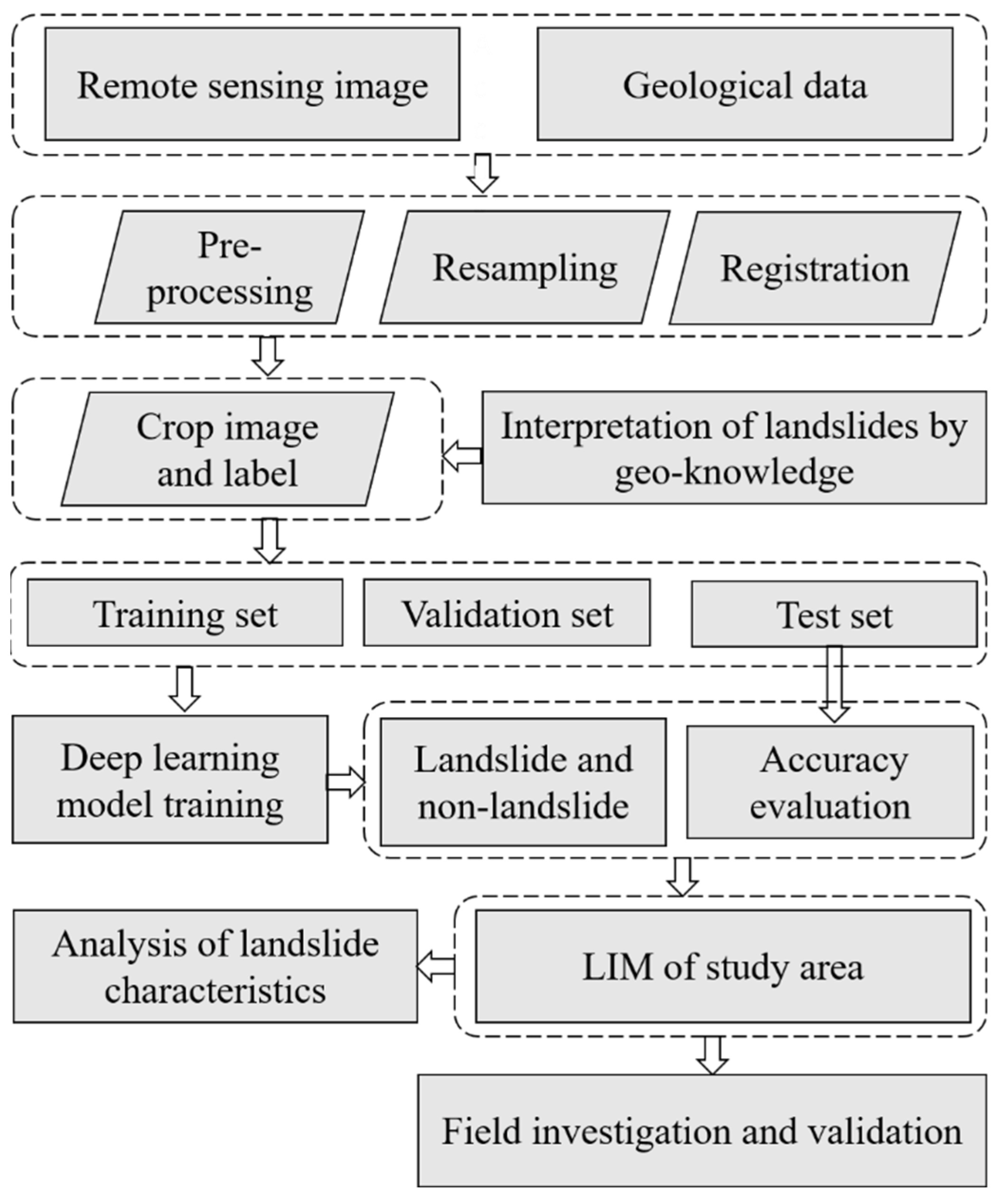
3.1. Content and Process of LIM

Landslide inventory mapping is a complex classification task that recognizes the size, shape, and distribution of landslides in a certain area using remote sensing image, geo-knowledge, and deep learning models. The process included three main steps (Figure 2): data pretreatment, classification, and accuracy evaluation; investigation and verification; and analysis.

In the first step, remote sensing images and geological data were preprocessed, including registration and resampling to the same resolution. Remote sensing images were preprocessed by atmospheric correction and radiometric correction. Landslides and non-landslides interpreted by geological knowledge were labels trained by deep learning models. Remote sensing images and labels were cropped in one-to-one correspondence. Images and corresponding label pairs were divided into training set, validation set, and test set. In the second step, images and labels were fed into the deep learning model for training. The network was mainly tuned by the training set. The loss value after each training iteration was obtained by the validation set to evaluate network quality. The test set was used to evaluate the accuracy of the trained network.

Finally, the results of LIM by image were verified through a field investigation to ensure accuracy. Simultaneously, the landslide distribution and typical characteristics were studied.

3.2. Overview of Imbalanced Sample LIM

In this study, the Bijie dataset was divided into training set, validation set, and test set. The training set was augmented through image processing. The imbalance ratio of the landslide sample was then reduced by augmentation. The samples and labels of the training set were flipped at different angles and filtered, blurred, and noisy. Subsequently, an FCN-FL network with a symmetric connection structure and focal loss was used. We added the level of network connections to increase feature level and suppress the influence of non-landslide samples on the model loss value (Figure 3). K-fold cross-validation was used to train the data to increase the robustness of the model and the utilization of the training set. The test set in the Bijie dataset was used to evaluate the network and the original FCN in this study. The landslide in Shuicheng County was used as a test set to evaluate the network and U-Net and SegNet in this study. Finally, Fa’er and Jichang Towns were used to obtain landslide inventory maps.

This study used remote sensing images of three areas: Bijie, Shuicheng, and Fa’er and Jichang. Detailed parameters are shown in

Table 1. Remote sensing image parameters in this study.

Area	Image	Acquisition Time	Resolution
Bijie	Google image	2019	0.8 m
Shuicheng	Google image	2021	1 m
Fa’er and Jichang	Sentinel-2	4 August 2021	10 m

. The Bijie dataset was based on Google Images published by Ji et al. This dataset included landslide images and corresponding landslide mask files. Google image was also used in the Shuicheng dataset to verify the improvement of our method. The Shuicheng dataset contained images and visual interpretation of landslide patterns. The Sentinel-2 images were used to obtain landslide inventory maps of Fa’er and Jichang Towns.

As for the processing of remote sensing images, we obtained Sentinel-2 images from the European Space Agency (https://scihub.copernicus.eu/dhus/ (accessed on 4 August 2021)). The Sen2Cor software was used for radiometric correction and atmospheric correction. Then, SNAP software was used for resampling, which was used as the input of the deep learning network.

3.3. Imbalance Ratio

The imbalance ratio parameter was used to measure the degree of sample imbalance, where D represents the collection of pixels of all training samples and each sample is represented by $\left(x,y\right)$, where $y\in \left\{0,1\right\}$. In this study, y values of 1 and 0 indicated that the pixel belonged to landslide and non-landslide, respectively.

Thus, the pixel set P of a landslide can be defined by Equation (1) and the non-landslide pixel set N as Equation (2). The imbalance ratio (IR) is defined as the ratio of non-landslide pixel number to landslide pixel number, as shown in Equation (3).

$$P=\left\{\left(x, y\right)| y=1\right\}, \left(x, y\right)\in D$$

(1)

$$N=\left\{\left(x, y\right)| y=0\right\}, \left(x, y\right)\in D$$

(2)

$$\mathrm{Imbalance}\mathrm{Ratio}\left(\mathrm{IR}\right)=\frac{\left|N\right|}{\left|P\right|}$$

(3)

According to Equation (3), IR is inversely proportional to the unbalanced degree of the dataset. To reduce the degree of imbalance of the dataset, the number of landslide samples in the data should be increased.

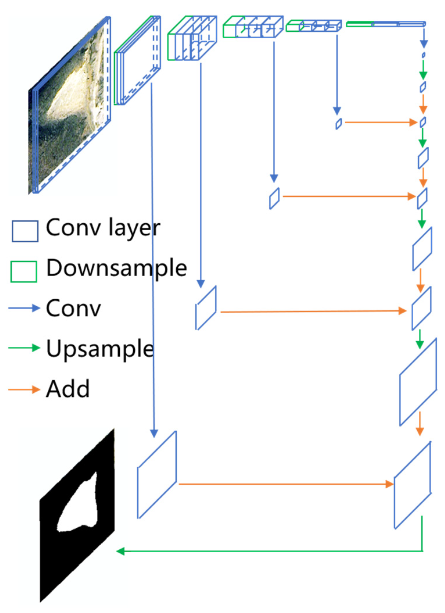
3.4. Fully Convolutional Networks (FCN)

Fully convolutional network is an end-to-end semantic segmentation network, which uses VGG16 as the backbone network and implements network training through feed-forward calculation and backpropagation. In Figure 4, the blue box represents the convolution layer of the learning sample features. The green box represents the lower sampling pooling layer. The green arrow is the upsampling operation, which matches the size of the feature graph with that of the upper level through upsampling and adds the data through the overlay operation of the orange arrow. The blue arrow represents the prediction result of the full-convolution operation. The prediction results of different depths were fused. To increase the feature level of the prediction, the convolution features of the first and second downsampling were added to the final prediction image.

The fully convolutional network undersampled by 5 times and extracted feature maps with five resolutions. The resolutions of the five downsampled feature maps were 1/2, 1/4, 1/8, 1/16, and 1/32 of the original image. This study added 1/2 and 1/4 of the feature maps connected to the upsampling compared to the original structure. These two feature maps with higher resolution provided rich details to distinguish landslide from non-landslide.

The FCN-FL adopts a fully connected symmetric structure to increase the scale of landslide feature extraction, which can improve the expression effect of the landslide boundary. Simultaneously, the focal loss function could be used to improve the contribution of landslide pixel to the model loss value and solve the problem of imbalanced samples that affect the accuracy of landslide recognition.

3.5. Focal Loss

Focal loss [42] is based on the cross entropy loss function (CE) [38], as shown in Equation (4), where Y is the pixel predicted value and 0 and 1 represent non-landslides and landslides, respectively.

$q\in \left[0,1\right]$ is the predicted value of the pixel. The predicted probability value is inversely proportional to the loss value.

$$\mathrm{CE}\left(q, y \right)=\left\{\begin{array}{c}-\log \left(q\right) y=1\\ -\log \left(1-q\right) y=0\end{array}\right.$$

(4)

Let $\mathrm{CE}\left(q, y \right)$ = $\mathrm{CE}\left(qt \right)$, which means $-\log \left(qt\right)$. The FL introduces two parameters, $\alpha$ and $\gamma$, as shown in Equation (5):

$$\mathrm{FL}\left(qt\right)=-\alpha {\left(1-qt\right)}^{\gamma }\log \left(qt\right)$$

(5)

The weight contributions of the landslide and non-landslide samples to the total loss are controlled by setting the value of $\alpha$. A low α value is used to reduce the weight of the non-landslide samples. ${\left(1-qt\right)}^{\gamma }$ is the focusing parameter, where $\gamma \ge 0$. By adjusting $\gamma$, the model focuses on difficult sample training. In this study, $\alpha$ and $\gamma$ were set to 0.25 and 1.75, respectively.

3.6. K-Fold Cross-Validation

K-fold cross-validation can reduce the negative impact of the training and validation sets on the model and improve the data utilization rate by taking full advantage of the sample data to participate in model training [43]. In this study, the original data D was randomly and averagely divided into five subsets of the same size, namely, D1, D2, …, D5, where four subsets were training sets, one subset was a verification set, and the verification set was not repeated, as shown in Figure 5. To evenly distribute the landslide and non-landslide samples in each dataset, labels 1 and 0 were assigned to landslide and non-landslide samples, respectively, during 5-fold cross-validation to ensure that random data division was based on the proportion of landslide and non-landslide samples.

3.7. Accuracy Evaluation

In the LIM task, each pixel was classified as either landslide or non-landslide. Thus, the four parameters of the confusion matrix were defined as true positive (TP), true negative (TN), false positive (FP), and false negative (FN). The TP refers to landslide output as landslide, TN refers to non-landslide output as non-landslide, FP refers to non-landslide output as landslide, and FN refers to landslide output as non-landslide.

Accuracy (Equation (6)), recall (Equation (7)), and F1-score (Equation (8)) were used to evaluate the accuracy of the model, and four parameters of the confusion matrix were used for the calculation.

$$\mathrm{Accuracy}=\frac{\mathrm{TP}+\mathrm{TN}}{\mathrm{TP}+\mathrm{FP}+\mathrm{TN}+\mathrm{FN}}$$

(6)

$$\mathrm{Recall}=\frac{\mathrm{TP}}{\mathrm{TP}+\mathrm{FN}}$$

(7)

$$\mathrm{F}1\mathrm{score}=\frac{2\times \mathrm{TP}}{2\times \mathrm{TP}+\mathrm{FP}+\mathrm{FN}}$$

(8)

The mean intersection over union (mIoU) (Equation (9)) was used to evaluate the ratio of intersection and union between the model prediction results and labels. The higher the ratio, the higher the accuracy. Here, q is the number of predicted categories. In this study, this value was 2.

$$\mathrm{mIoU}=\frac{1}{q+1}{\displaystyle \sum }_{i=0}^q\frac{\mathrm{TP}}{\mathrm{TP}+\mathrm{FP}+\mathrm{FN}}$$

(9)

4. Results

4.1. Landslide Sample Augmentation

There were 770 landslides and 2003 non-landslides samples collected in Bijie City. The sample size was resized to 256 × 256 pixels. As the non-landslide samples in the Bijie landslide dataset had no corresponding labels, labels for non-landslides were added. The sample imbalance ratio was then calculated by counting the number of landslide and non-landslide pixels in the Bijie landslide dataset (

Table 2. Imbalance ratio comparison before and after landslide sample augmentation.

	Before	After
Landslide	$2\times {10}^7$	$8\times {10}^7$
Non-landslide	$1.6\times {10}^8$	2.5 $\times {10}^8$
IR	8	3.1

).

Data augmentation methods include image flipping, blur adjustment, and noise increase. In this study, a left–right flip with mean filter, an up–down flip with random gamma stretch, and a mirror flip with random noise were applied to the image. Lines a, b, and c in Figure 6 correspond to the above three operations. The left and right images in each group are the original and augmented images, respectively.

4.2. Prediction Results of FCN-FLK, FCN-FL, and FCN in the Bijie Dataset

In this study, 70 landslide samples were selected as the test data. The remaining 700 samples and enhanced landslide and non-landslide samples were used as the training data. The training data consisted of a training set and a verification set. A total of 80% of the original landslide, augmented landslide, and non-landslide samples were used as training set and 20% as verification set.

For a small sample size of dataset, the FCN-FL model (FCN-FLK) was trained using the 5-fold cross-validation method to effectively use all the data. The K-fold cross-validation method randomly divides data into K equal parts, selects one part as the verification set, and uses the remaining data as the training set. The iterative training for K times can effectively use all the data to train the model. In this study, the data were evenly divided into five groups. To evenly divide the landslide and non-landslide data, labels 1 and 0 were assigned to the samples, respectively. The data were then divided according to the proportion of landslides and non-landslides in the samples.

Accuracy, recall, and F1-score were used to evaluate the model accuracy, and mIoU was used to evaluate the prediction results.

The performance of the FCN-FLK model was superior to those of the FCN-FL and FCN models in terms of model accuracy and prediction results (

Table 3. Statistical accuracies of FCN-FLK, FCN-FL, and FCN.

	FCN-FLK	FCN-FL	FCN
Accuracy	0.93	0.92	0.87
Recall	0.76	0.73	0.68
F1-score	0.62	0.58	0.53
mIoU	0.68	0.66	0.53

). Compared to the FCN model, the recall, F1-score, and mIoU of the FCN-FL model were improved by 0.05, 0.05, and 0.13, respectively. This proves that symmetric connection can improve the accuracy of the model in identifying landslide boundaries. Compared to the FCN model, focal loss improved the contribution of landslide samples to the loss value of the whole model by controlling the weight of the landslide and non-landslide samples. The classification accuracy was further improved by focusing on the training of hard-to-classify samples with focal parameters. The recall, F1-score, and mIoU of the FCN-FLK model were improved by 0.08, 0.09, and 0.15, respectively. The comparison in Figure 7 shows that the identification results of the FCN-FLK model had high similarity, demonstrating that the K-fold cross-validated FCN-FL model had better robustness. The FCN and FCN-FL models could misjudge bare soil and roads with similar characteristics around landslides, while FCN-FLK had less missed judgment (FP) and less wrong judgment (TN).

4.3. Comparison of FCN-FLK, SegNet, and U-NET Models

A landslide inventory map of Liupanshui City from 2019 was obtained. The Bijie landslide data are RGB images with a resolution of 0.8 m. To match the sample data, Google images from 2021 with a resolution of 1 m were selected. A total of 146 landslide points were obtained from the landslide data of Shuicheng County. Landslide points with indistinct geomorphic features and vegetation-covered surfaces were deleted. Simultaneously, new landslide points that have occurred since 2019 were added. Figure 8 shows the distribution map of the landslide points in Shuicheng County.

The FCN-FLK model was used to obtain landslide data from Shuicheng County to verify the generalization of the model. Meanwhile, the U-Net [44] and SegNet [45] models were trained using the training data and validation data introduced in Section 3.2, and the same VGG16 network as the FCN was used as the backbone network. The accuracy, recall, F1-score, and mIoU of the four models were calculated, as shown in

Table 4. Comparison of accuracy for FCN-FL, U-Net, and SegNet.

	FCN-FLK	U-Net	SegNet
Accuracy	0.93	0.90	0.89
Recall	0.76	0.68	0.64
F1-score	0.62	0.53	0.44
mIoU	0.68	0.63	0.59

.

The FCN-FLK model outperformed the traditional SegNet and U-Net networks, with recall and F1-score being significantly better than SegNet [46] (Table 4). The segmentation accuracy mIoU of the FCN-FLK model was also improved. Figure 9 shows that the shape of the FCN-FLK segmentation was closer to that of the label boundary of the visual interpretation. The SegNet model missed more parts of the segmentation, whereas the U-Net [35] model suffered from serious misjudgment.

4.4. LIM of Fa’er and Jichang Towns

The images of the study area (Figure 8) were input to test the performance of the FCN-FLK model in the regional LIM. Sentinel-2 images acquired on 4 August 2021 were preprocessed for radiometric correction and atmospheric correction. To maintain the same image resolution as the Bijie landslide samples, Sentinel-2 images were resampled to 1 m in green, blue, and red (2/3/4 band).

Figure 10 shows the LIM obtained using FCN-FLK (Figure 10a) and U-Net (Figure 10b). Shuicheng County is the area with the most serious geological disasters in Liupanshui, whereas Fa’er and Jichang Towns have experienced large landslides every year from 2018 to 2021. Therefore, this area was selected as the research subject for the LIM test. The false and missed detections of the FCN-FLK model were less than those of U-NET, indicating that the FCN-FLK model was more efficient in the large-scale landslide inventory map (Figure 10). According to the visual comparison in the blue box in Figure 10, the FCN-FLK model had a low misjudgment rate in the non-landslide area, which could reduce the workload of visual interpretation to remove misjudgment and improve the efficiency of LIM.

Owing to the complex background of historical landslides, some false detections occur in the bare soil. These areas are similar in shape to landslides, leading to false detection. False detections can be eliminated by visual interpretation in the final result. Most landslides occur in areas with slopes greater than 15°. The LIM results might have been better if the non-landslide in the Bijie dataset included DEM data.

Figure 11 shows the comparison of the model identification and visual interpretation results of the three landslides in the study area in 2018, 2019, and 2021. Landslide I is the Jianshanying landslide, in which landslide (a) occurred in 2018. The landslide boundary of landslide (a) can be clearly seen by comparing the two GF-2 images from March 2018 and December 2018 in Figure 11c,d. In Figure 11a, landslide (a) was completely identified, whereas only part of the area was identified in Figure 11b. The identification result of landslide (b) in I was relatively inaccurate because landslide (b) was potentially caused by mining. The surface of (b) was relatively broken and in the stage of continuous massive deformation under the action of underground mining. As there was no large-scale overall slip, the surface features were relatively complex, resulting in poor identification results. Landslide II was a large landslide in Jichang Town on 23 July 2019, which caused huge property losses. It can be seen from Figure 11j,h that a large amount of material migration occurred on the surface of the landslide with a clear boundary. The identification results in Figure 11e are good, whereas those in Figure 11f are inaccurate. Landslide III is the landslide in Jingtou Village, Jichang Town, that occurred on 15 July 2021. Owing to timely warning and successful avoidance, no casualties occurred. Figure 11k,l shows that although the landslide caused material damage, the toppled houses were still in the original area. Therefore, some regions were not identified in Figure 11i, whereas they were not identified at all in Figure 11j.

4.5. Field Investigation

To verify the results of landslide inventory, the research team conducted a field survey of the Jianshanying landslide (landslide I in Figure 11) in Fa’er Town in September 2021. Figure 12a,b shows the tableland of the landslide. As shown in Figure 12a, there were evident tensile cracks on the tableland of the landslide. Figure 12b shows the fractured surface caused by the slope movement. Figure 12c shows an overall picture of the landslide taken at the foot of the slope, where there are residential buildings and the risk of landslides is high.

5. Discussion

It has been proven that the convolutional neural network approach significantly outperforms traditional machine learning methods in landslide inventory mapping. However, there still exist sample problems in the application of convolutional neural network in landslide inventory mapping. The convolutional neural network needs a large number of samples to improve the robustness of the network. However, in most cases, the number of landslide samples is not enough. At the same time, they are sparse in the distribution of natural features. To this end, we proposed a 5-fold cross-validation method to improve the sample utilization rate. The focus loss increased the contribution value of landslide samples in the loss function and made the network focus on the learning of landslide samples. In Section 4.2 and Section 4.3, we proved that our proposed focus loss FCN (FCN-FL) outperformed the traditional FCN network and two common semantic segmentation networks (U-Net [1] and SegNet [2]). In the experiment, the proposed method could improve the sample utilization rate and obtained better landslide inventory mapping of Fa’er and Jichang Towns (Section 4.4).

6. Conclusions

In this study, a landslide inventory method for sample disequilibrium was proposed. The validity of the method was verified by the data source, model optimization, and training methods. The full CNN was adopted as the basic model, which adds the corresponding channels of the feature map to increase the information content of the feature map. It is better suited for historical landslide cataloguing with fuzzy boundaries and complex backgrounds. The focus loss function, which focuses on the training of difficult samples, inhibits the loss value contribution of negative samples to the model and improves the accuracy of the model. Results showed that the accuracy of the FCN-FL model was better than that of the FCN model. The training method of 5-fold cross-validation further improved the robustness of the model and the data utilization rate of the landslide dataset with small samples. The 5-fold cross-validation ensured that 20% of the dataset was used as the validation set, which avoided the influence of the accuracy of the validation set and the loss function value on the model in the training process. It was further verified that the 5-fold cross-validation model was more robust than FCN-FL.

Here, data augmentation was used to reduce the degree of sample imbalance. In addition, the 5-fold cross-validation improved the robustness of the model. By comparing the prediction accuracy of the FCN and FCN-FL models in the Bijie dataset, it was found that the FCN-FL model could improve the recognition accuracy of the landslide boundary by adding feature layers. The recognition image was more complete than that of FCN. The FCN-FL model had better generalization and segmentation accuracy than the SegNet and U-NET models for landslide data recognition in Shuicheng County. The FCN-FL model was also relatively complete for the boundary extraction of landslides. This research provides a reference for addressing imbalanced samples in the deep learning of LIM.

In this study, landslide sites were easily detected in areas with large vegetation coverage. However, detection remains a challenge in areas with little vegetation cover. The boundary between landslides and bare soil is not obvious and is even difficult to interpret visually. Further research will focus on the diversity of landslide samples and the extension of the model.

References

1. Peng, J.; Fan, Z.; Wu, D.; Zhuang, J.; Dai, F.; Chen, W.; Zhao, C. Heavy Rainfall Triggered Loess–Mudstone Landslide and Subsequent Debris Flow in Tianshui, China. Eng. Geol. 2015, 186, 79–90. [Google Scholar] [CrossRef]
2. Mohan, A.; Singh, A.K.; Kumar, B.; Dwivedi, R. Review on Remote Sensing Methods for Landslide Detection Using Machine and Deep Learning. Trans. Emerg. Telecommun. Technol. 2021, 32, e3998. [Google Scholar] [CrossRef]
3. Guzzetti, F.; Mondini, A.C.; Cardinali, M.; Fiorucci, F.; Santangelo, M.; Chang, K.-T. Landslide Inventory Maps: New Tools for an Old Problem. Earth-Sci. Rev. 2012, 112, 42–66. [Google Scholar] [CrossRef] [Green Version]
4. Harp, E.L.; Keefer, D.K.; Sato, H.P.; Yagi, H. Landslide Inventories: The Essential Part of Seismic Landslide Hazard Analyses. Eng. Geol. 2011, 122, 9–21. [Google Scholar] [CrossRef]
5. Zhao, C.; Lu, Z. Remote Sensing of Landslides—A Review. Remote Sens. 2018, 10, 279. [Google Scholar] [CrossRef] [Green Version]
6. Temme, A.; Guzzetti, F.; Samia, J.; Mirus, B.B. The Future of Landslides’ Past—A Framework for Assessing Consecutive Landsliding Systems. Landslides 2020, 17, 1519–1528. [Google Scholar] [CrossRef]
7. Yordanov, V.; Biagi, L.; Truong, X.Q.; Tran, V.A.; Brovelli, M.A. An Overview of Geoinformatics State-of-the-Art Techniques for Landslide Monitoring and Mapping. Int. Arch. Photogramm. Remote Sens. Spat. Inf. Sci. 2021, XLVI-4/W2-2021, 205–212. [Google Scholar] [CrossRef]
8. Fiorucci, F.; Giordan, D.; Santangelo, M.; Dutto, F.; Rossi, M.; Guzzetti, F. Criteria for the Optimal Selection of Remote Sensing Optical Images to Map Event Landslides. Nat. Hazards Earth Syst. Sci. 2018, 18, 405–417. [Google Scholar] [CrossRef] [Green Version]
9. Zhang, L.; Zhang, L.; Du, B. Deep Learning for Remote Sensing Data: A Technical Tutorial on the State of the Art. IEEE Geosci. Remote Sens. Mag. 2016, 4, 22–40. [Google Scholar] [CrossRef]
10. Zhong, C.; Liu, Y.; Gao, P.; Chen, W.; Li, H.; Hou, Y.; Nuremanguli, T.; Ma, H. Landslide Mapping with Remote Sensing: Challenges and Opportunities. Int. J. Remote Sens. 2020, 41, 1555–1581. [Google Scholar] [CrossRef]
11. Tian, Y.; Xu, C.; Ma, S.; Xu, X.; Wang, S.; Zhang, H. Inventory and Spatial Distribution of Landslides Triggered by the 8th August 2017 MW 6.5 Jiuzhaigou Earthquake, China. J. Earth Sci. 2019, 30, 206–217. [Google Scholar] [CrossRef]
12. Hervás, J.; Barredo, J.I.; Rosin, P.L.; Pasuto, A.; Mantovani, F.; Silvano, S. Monitoring Landslides from Optical Remotely Sensed Imagery: The Case History of Tessina Landslide, Italy. Geomorphology 2003, 54, 63–75. [Google Scholar] [CrossRef]
13. Mondini, A.C.; Guzzetti, F.; Reichenbach, P.; Rossi, M.; Cardinali, M.; Ardizzone, F. Semi-Automatic Recognition and Mapping of Rainfall Induced Shallow Landslides Using Optical Satellite Images. Remote Sens. Environ. 2011, 115, 1743–1757. [Google Scholar] [CrossRef]
14. Li, Z.; Shi, W.; Myint, S.W.; Lu, P.; Wang, Q. Semi-Automated Landslide Inventory Mapping from Bitemporal Aerial Photographs Using Change Detection and Level Set Method. Remote Sens. Environ. 2016, 175, 215–230. [Google Scholar] [CrossRef]
15. Siyahghalati, S.; Saraf, A.K.; Pradhan, B.; Jebur, M.N.; Tehrany, M.S. Rule-Based Semi-Automated Approach for the Detection of Landslides Induced by 18 September 2011 Sikkim, Himalaya, Earthquake Using IRS LISS3 Satellite Images. Geomat. Nat. Hazards Risk 2016, 7, 326–344. [Google Scholar] [CrossRef] [Green Version]
16. Ramos-Bernal, R.; Vázquez-Jiménez, R.; Romero-Calcerrada, R.; Arrogante-Funes, P.; Novillo, C. Evaluation of Unsupervised Change Detection Methods Applied to Landslide Inventory Mapping Using ASTER Imagery. Remote Sens. 2018, 10, 1987. [Google Scholar] [CrossRef] [Green Version]
17. Yang, W.; Wang, Y.; Sun, S.; Wang, Y.; Ma, C. Using Sentinel-2 Time Series to Detect Slope Movement before the Jinsha River Landslide. Landslides 2019, 16, 1313–1324. [Google Scholar] [CrossRef]
18. Parker, R.N.; Densmore, A.L.; Rosser, N.J.; de Michele, M.; Li, Y.; Huang, R.; Whadcoat, S.; Petley, D.N. Mass Wasting Triggered by the 2008 Wenchuan Earthquake Is Greater than Orogenic Growth. Nat. Geosci. 2011, 4, 449–452. [Google Scholar] [CrossRef] [Green Version]
19. Dou, J.; Chang, K.-T.; Chen, S.; Yunus, A.; Liu, J.-K.; Xia, H.; Zhu, Z. Automatic Case-Based Reasoning Approach for Landslide Detection: Integration of Object-Oriented Image Analysis and a Genetic Algorithm. Remote Sens. 2015, 7, 4318–4342. [Google Scholar] [CrossRef] [Green Version]
20. Behling, R.; Roessner, S.; Kaufmann, H.; Kleinschmit, B. Automated Spatiotemporal Landslide Mapping over Large Areas Using RapidEye Time Series Data. Remote Sens. 2014, 6, 8026–8055. [Google Scholar] [CrossRef]
21. Stumpf, A.; Lachiche, N.; Malet, J.-P.; Kerle, N.; Puissant, A. Active Learning in the Spatial Domain for Remote Sensing Image Classification. IEEE Trans. Geosci. Remote Sens. 2014, 52, 2492–2507. [Google Scholar] [CrossRef]
22. Tien Bui, D.; Shahabi, H.; Shirzadi, A.; Chapi, K.; Alizadeh, M.; Chen, W.; Mohammadi, A.; Ahmad, B.; Panahi, M.; Hong, H.; et al. Landslide Detection and Susceptibility Mapping by AIRSAR Data Using Support Vector Machine and Index of Entropy Models in Cameron Highlands, Malaysia. Remote Sens. 2018, 10, 1527. [Google Scholar] [CrossRef] [Green Version]
23. Stumpf, A.; Malet, J.-P.; Delacourt, C. Correlation of Satellite Image Time-Series for the Detection and Monitoring of Slow-Moving Landslides. Remote Sens. Environ. 2017, 189, 40–55. [Google Scholar] [CrossRef]
24. Yuan, Q.; Shen, H.; Li, T.; Li, Z.; Li, S.; Jiang, Y.; Xu, H.; Tan, W.; Yang, Q.; Wang, J.; et al. Deep Learning in Environmental Remote Sensing: Achievements and Challenges. Remote Sens. Environ. 2020, 241, 111716. [Google Scholar] [CrossRef]
25. Ma, Z.; Mei, G. Deep Learning for Geological Hazards Analysis: Data, Models, Applications, and Opportunities. Earth-Sci. Rev. 2021, 223, 103858. [Google Scholar] [CrossRef]
26. Chen, Z.; Zhang, Y.; Ouyang, C.; Zhang, F.; Ma, J. Automated Landslides Detection for Mountain Cities Using Multi-Temporal Remote Sensing Imagery. Sensors 2018, 18, 821. [Google Scholar] [CrossRef] [Green Version]
27. Franklin, S.E. Interpretation and Use of Geomorphometry in Remote Sensing: A Guide and Review of Integrated Applications. Int. J. Remote Sens. 2020, 41, 7700–7733. [Google Scholar] [CrossRef]
28. Ji, S.; Yu, D.; Shen, C.; Li, W.; Xu, Q. Landslide Detection from an Open Satellite Imagery and Digital Elevation Model Dataset Using Attention Boosted Convolutional Neural Networks. Landslides 2020, 17, 1337–1352. [Google Scholar] [CrossRef]
29. Lei, T.; Zhang, Y.; Lv, Z.; Li, S.; Liu, S.; Nandi, A.K. Landslide Inventory Mapping From Bitemporal Images Using Deep Convolutional Neural Networks. IEEE Geosci. Remote Sens. Lett. 2019, 16, 982–986. [Google Scholar] [CrossRef]
30. Ju, Y.; Xu, Q. Automatic Objection of Loess Landslide Based on Deep Learning. Geomat. Inf. Sci. Wuhan Univ. 2020, 45, 1747–1755. [Google Scholar]
31. Jiang, W.; Xi, J.; Li, Z.; Ding, M.; Yang, L.; Xie, D. Landslide Detection and Segmentation Using Mask R-CNN with Simulated Hard Samples. Geomat. Inf. Sci. Wuhan Univ. 2022, 1–18. [Google Scholar] [CrossRef]
32. Prakash, N.; Manconi, A.; Loew, S. Mapping Landslides on EO Data: Performance of Deep Learning Models vs. Traditional Machine Learning Models. Remote Sens. 2020, 12, 346. [Google Scholar] [CrossRef] [Green Version]
33. Ghorbanzadeh, O.; Blaschke, T.; Gholamnia, K.; Meena, S.; Tiede, D.; Aryal, J. Evaluation of Different Machine Learning Methods and Deep-Learning Convolutional Neural Networks for Landslide Detection. Remote Sens. 2019, 11, 196. [Google Scholar] [CrossRef] [Green Version]
34. Qi, W.; Wei, M.; Yang, W.; Xu, C.; Ma, C. Automatic Mapping of Landslides by the ResU-Net. Remote Sens. 2020, 12, 2487. [Google Scholar] [CrossRef]
35. Liu, P.; Wei, Y.; Wang, Q.; Chen, Y.; Xie, J. Research on Post-Earthquake Landslide Extraction Algorithm Based on Improved U-Net Model. Remote Sens. 2020, 12, 894. [Google Scholar] [CrossRef] [Green Version]
36. Gao, X.; Chen, T.; Niu, R.; Plaza, A. Recognition and Mapping of Landslide Using a Fully Convolutional DenseNet and Influencing Factors. IEEE J. Sel. Top. Appl. Earth Obs. Remote Sens. 2021, 14, 7881–7894. [Google Scholar] [CrossRef]
37. Shi, W.; Zhang, M.; Ke, H.; Fang, X.; Zhan, Z.; Chen, S. Landslide Recognition by Deep Convolutional Neural Network and Change Detection. IEEE Trans. Geosci. Remote Sens. 2021, 59, 4654–4672. [Google Scholar] [CrossRef]
38. Lin, T.-Y.; Goyal, P.; Girshick, R.; He, K.; Dollar, P. Focal Loss for Dense Object Detection. IEEE Trans. Pattern Anal. Mach. Intell. 2020, 42, 318–327. [Google Scholar] [CrossRef] [Green Version]
39. Wang, J.; Li, F.; Bi, H. Gaussian Focal Loss: Learning Distribution Polarized Angle Prediction for Rotated Object Detection in Aerial Images. IEEE Trans. Geosci. Remote Sens. 2022, 60, 1–13. [Google Scholar] [CrossRef]
40. Liu, Y.; Pang, C.; Zhan, Z.; Zhang, X.; Yang, X. Building Change Detection for Remote Sensing Images Using a Dual-Task Constrained Deep Siamese Convolutional Network Model. IEEE Geosci. Remote Sens. Lett. 2021, 18, 811–815. [Google Scholar] [CrossRef]
41. Shelhamer, E.; Long, J.; Darrell, T. Fully Convolutional Networks for Semantic Segmentation. IEEE Trans. Pattern Anal. Mach. Intell. 2017, 39, 640–651. [Google Scholar] [CrossRef] [PubMed]
42. Jing, X.-Y.; Zhang, X.; Zhu, X.; Wu, F.; You, X.; Gao, Y.; Shan, S.; Yang, J.-Y. Multiset Feature Learning for Highly Imbalanced Data Classification. IEEE Trans. Pattern Anal. Mach. Intell. 2021, 43, 139–156. [Google Scholar] [CrossRef] [PubMed]
43. Meena, S.R.; Ghorbanzadeh, O.; van Westen, C.J.; Nachappa, T.G.; Blaschke, T.; Singh, R.P.; Sarkar, R. Rapid Mapping of Landslides in the Western Ghats (India) Triggered by 2018 Extreme Monsoon Rainfall Using a Deep Learning Approach. Landslides 2021, 18, 1937–1950. [Google Scholar] [CrossRef]
44. Falk, T.; Mai, D.; Bensch, R.; Özgün, Ç. U-Net: Deep Learning for Cell Counting, Detection, and Morphometry. Nat. Methods 2019, 16, 67–70. [Google Scholar] [CrossRef]
45. Badrinarayanan, V.; Kendall, A.; Cipolla, R. SegNet: A Deep Convolutional Encoder-Decoder Architecture for Image Segmentation. IEEE Trans. Pattern Anal. Mach. Intell. 2017, 39, 2481–2495. [Google Scholar] [CrossRef]
46. Yu, B.; Chen, F.; Xu, C.; Wang, L.; Wang, N. Matrix SegNet: A Practical Deep Learning Framework for Landslide Mapping from Images of Different Areas with Different Spatial Resolutions. Remote Sens. 2021, 13, 3158. [Google Scholar] [CrossRef]
Figure 1. Background of the study area. The locations of Shuicheng County and Fa’er and Jichang Towns are shown in the figure. The blue point represents the landslide distribution of the Bijie dataset.
Remotesensing 14 05517 g001
Figure 2. Flow chart of landslide inventory mapping.
Remotesensing 14 05517 g002
Figure 3. Flowchart of the imbalanced landslide inventory mapping.
Remotesensing 14 05517 g003
Figure 4. Architecture of FCN for imbalanced landslide inventory mapping.
Remotesensing 14 05517 g004
Figure 5. Flow chart of the K-fold cross-validation.
Remotesensing 14 05517 g005
Figure 6. Exemplary figures of landslide sample augmentation. (a1a3) Images processed by left–right flip with mean filter; (b1b3) images processed by up–down flip with random gamma stretch; (c1c3) images processed by mirror flip with random noise.
Remotesensing 14 05517 g006
Figure 7. Comparison of FCN, FCN-FL, and FCN-FLK prediction results on the Bijie landslide dataset. Purple, red, and blue represent true positive, false positive, and true negative, respectively. (a,e,i) Original images; (b,f,j) results of FCN-FLK; (c,g,k) results of FCN-FL; (d,h,l) results of FCN.
Remotesensing 14 05517 g007
Figure 8. Landslides distribution in Shuicheng County.
Remotesensing 14 05517 g008
Figure 9. Prediction of landslides in Shuicheng County using FCN-FL, U-Net, and SegNet. Brown, red, and yellow represent true positive, false positive, and true negative, respectively. (a,e,i) Original images; (b,f,j) results of FCN-FLK; (c,g,k) results of U-Net; (d,h,l) results of SegNet.
Remotesensing 14 05517 g009
Figure 10. Landslide inventory maps of Fa’er and Jichang Towns using FCN-FLK and U-Net. (a,b) are the prediction results of FCN-FLK and U-Net, respectively. Blue boxes indicate false detections. Symbol I to III are the details of three remote sensing images, as shown in Figure 11.
Remotesensing 14 05517 g010
Figure 11. Landslides recognition results with different segmentation methods and visual interpretation in Shuicheng County in 2018, 2019, and 2021. (a,e,i) results of FCN-FLK; (b,f,j) results of U-Net; (c,d) GF-2 image of landslide I; (g,h) photo of landslide II; (k,l) photo of landslide III.
Remotesensing 14 05517 g011
Figure 12. Field geological survey of Jianshanying landslide in Shuicheng County. (a) A crack; (b) the fracture surface; (c) the overall picture of the landslide.
Remotesensing 14 05517 g012