Abstract
Predicting the shape evolution and movement of remote sensing satellite cloud images is a difficult task requiring the effective monitoring and rapid prediction of thunderstorms, gales, rainstorms, and other disastrous weather conditions. We proposed a generative adversarial network (GAN) model for time series satellite cloud image prediction in this research. Taking time series information as the constraint condition and abandoning the assumption of linear and stable changes in cloud clusters in traditional methods, the GAN model is used to automatically learn the data feature distribution of satellite cloud images and predict time series cloud images in the future. Through comparative experiments and analysis, the Mish activation function is selected for integration into the model. On this basis, three improvement measures are proposed: (1) The Wasserstein distance is used to ensure the normal update of the GAN model parameters; (2) establish a multiscale network structure to improve the long-term performance of model prediction; (3) combined image gradient difference loss (GDL) to improve the sharpness of prediction cloud images. The experimental results showed that for the prediction cloud images of the next four times, compared with the unimproved Mish-GAN model, the improved GDL-GAN model improves the PSNR and SSIM by 0.44 and 0.02 on average, and decreases the MAE and RMSE by 18.84% and 7.60% on average. It is proven that the improved GDL-GAN model can maintain good visualization effects while keeping the overall changes and movement trends of the prediction cloud images relatively accurate, which is helpful to achieve more accurate weather forecast. The cooperation ability of satellite cloud images in disastrous weather forecasting and early warning is enhanced.
1. Introduction
Disastrous weather forecasts are very important information in daily life, and research on real-time and accurate disastrous weather forecasts is also essential. In areas with complex terrain and extremely harsh environments, it is difficult and costly to build traditional meteorological observation stations. Meteorological satellites can obtain data all day by means of remote sensing, which has great advantages in observation and prediction compared with traditional methods. Satellite cloud images can provide the information on cloud shape, movement trajectories, generation, and dissipation, thereby providing sufficient and valuable information for the overall study of cloud images and subsequent meteorological assessment and forecasting [1,2,3].
The early satellite cloud image prediction method was mainly based on the matching and tracking of cloud clusters. By determining specific cloud clusters, the movement of cloud clusters is observed and inferred. Zinner et al. [4] used three kinds of satellite data combined with vector fields to predict the drift of cloud clusters based on the overlap between the current frame and the next frame. Jamaly et al. [5] used cross-correlation and cross-spectrum analysis to estimate cloud motion and added additional quality control measures to improve the reliability of cloud motion estimation. Shi et al. [6] extrapolated infrared satellite cloud images by using a dense optical flow model combined with the DIS optical flow algorithm and backward advection scheme. Dissawa [7] proposed a method for tracking and predicting cloud motion using cross-correlation and optical flow methods for ground-based sky images. The above studies are based on the static characteristics of cloud cluster changes, ignoring nonstationary changes such as cloud cluster turnover during atmospheric movement, which limits the practicability and scientificity of cloud image prediction.
To meet the complex characteristics of cloud clusters, an increasing number of scholars have proposed nonlinear cloud image prediction technology. Liang et al. [8] combined cellular automata with the growth and movement characteristics of cloud images and proposed a short-term prediction method for cloud images based on cellular automata. Pang [9] used the k-means algorithm to establish a cloud movement pattern recognition model, based on which a patch-matching algorithm, a feature-matching algorithm, and an optical flow algorithm were combined to predict the movement of clouds. Wang et al. [10] used cubic spline interpolation function fitting to realize dynamic tracking prediction of cloud images according to the cyclone theory of cloud cluster movement. These methods are highly scientific and require many mathematical operations as support. As an implicitly complex function, neural networks are good at simulating complex dynamic systems [11], which provide great potential in the application of satellite cloud image prediction. He et al. [12] used the combination of EOF expansion and a neural network to perform spatiotemporal inversion of time coefficients and spatial feature vectors to predict cloud images. Jin et al. [13] adopted an ensemble prediction method similar to a numerical prediction model and constructed a nonlinear prediction model of satellite cloud images based on a genetic neural network. Penteliuc [14] obtained the motion vector flow from the cloud mask sequence by the optical flow method, and trained the cloud image prediction model based on a multilayer perceptron. Huang et al. [15] constructed a nonlinear intelligent prediction model of typhoon satellite cloud images based on the cooperative strategy Shapley-fuzzy neural network.
As a rising star in the field of deep learning, generative adversarial networks (GAN) [16] are one of the most representative unsupervised networks and are widely used in image generation [17], video prediction [18], and other fields. Yan et al. [19] built a conditional GAN model for human motion image prediction by taking human skeleton frame information as a constraint condition. Xu et al. [20] proposed a GAN-LSTM model for FY-2E satellite cloud image prediction by combining the generation ability of GAN and the prediction ability of LSTM. Therefore, using the time series satellite cloud images as a data-driven, combined with the GAN, model to automatically learn and infer the meteorological information contained in the satellite cloud images, the satellite cloud images are quickly and accurately predicted and outputted at the future times, eliminating the steps of image feature preextraction before model training, and saving human resources.
Based on GAN, this paper constructs a FY-4A time series satellite cloud image prediction model. On the basis of selecting the activation function with the best prediction effect, three improvement measures are proposed for the time series satellite cloud images prediction GAN model: Wasserstein distance is used to realize the “adversarial” training of the model; using a multiscale network structure to improve the long-term performance of model prediction; image gradient difference loss is introduced to enhance the sharpness of predicted cloud images. The experimental results demonstrate the effectiveness of the improved scheme, and the accuracy of predicting the overall change and movement trend of the sequence cloud images is significantly improved.
2. Construction and Analysis of a Time Series Cloud Images Prediction Model Based on GAN
2.1. Construction of the Time Series Cloud Images Dataset
In the application and scientific research of satellite cloud image, the main research objects are visible cloud image and infrared cloud image. Compared with the infrared and visible cloud images, the water vapor cloud image can show the details of the weather system earlier, more completely and more continuously, and is basically not affected by the diurnal variation, which can more truly reflect the occurrence and development of the weather system and its change process with time. Comprehensive analysis, this paper selected FY-4A water vapor cloud image as the research object, to carry out time series cloud images prediction.
The experimental data are from the FY-4A water vapor cloud image of China released by the National Satellite Meteorological Center (NSMC). The images are processed by calibration data standardization, parameter correction, and brightness temperature model. An image instance is depicted in Figure 1. A total of 720 original images was selected for the experiment, which lasted for 30 days with an interval of 1 h. The training set and the test set are allocated in a 5:1 ratio. The data overview is shown in Table 1.
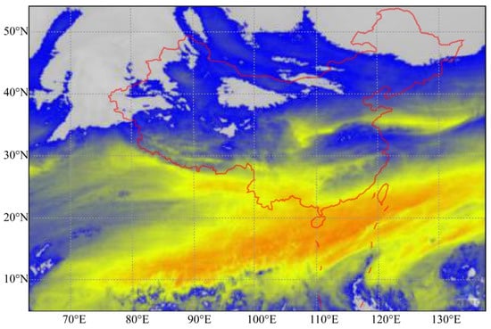
Figure 1.
China regional FY-4A water vapor cloud image.

Table 1.
Overview of the water vapor cloud image.
Due to the large coverage of a single image and the complex variation of the cloud image within the same frame, the original images are cropped in a row-column order of 64 × 64 size during the production of the training set, ensuring that the spatial range does not overlap. The 600 small images of the same geographical location obtained by splitting are used as a cube combination, for a total of 504 cube combinations, the process is shown in Figure 2a. After that, each cube combination is used to extract the sample sequence, the extraction process is shown in Figure 2b. For each cube combination, starting from 0:00 on April 16, the images are continuously intercepted as a single sample sequence in an 8-h cycle. There was no time repetition between each sample sequence. At the same time, the L2 difference of adjacent time images in each sample sequence is compared, so as to quantitatively screen the sample sequence, and ensure that each sequence has enough moving changes. About 30,000 sample sequences are selected as the training set. We make a 400 × 400 size test set in the same way, with a total of 100 sample sequences.
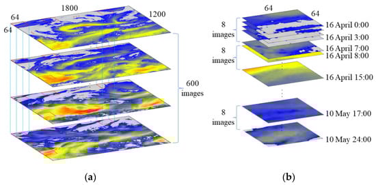
Figure 2.
Time series cloud image dataset diagram: (a) cube combination segmentation diagram and (b) sample sequence extraction diagram.
2.2. Construction of a Time Series Cloud Images Prediction Model Based on GAN
In this paper, by limiting the input samples to satellite cloud images of the first four times, the time series information is used by inputting the GAN model along the time series, and the size is set to a fixed value of 64 × 64 to ensure that the prediction results are consistent with the input size. The satellite cloud images of the next four times are predicted. The model structure is shown in Figure 3.
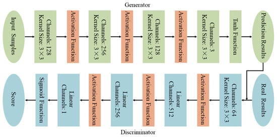
Figure 3.
GAN model structure diagram for the prediction of time series cloud images.
It is assumed that the input sequence samples at the first four times are X, and the real results at the next four times are Y. The generator takes X as input, first enters the convolution layer, extracts features through the convolution operation, and pads the edges of the input matrix in the convolution process so that its output maintains the size before the convolution operation. Then, entering the activation layer, the activation function is introduced to nonlinearly change the feature matrix after convolution. The receptive field is increased by multilayer convolution, and the temporal variation characteristics of images at different levels are extracted. After the last layer of convolution processing, the Tanh function layer is connected to activate the function, and the generated image is normalized. At this time, the generator image generation process is completed, and the generated prediction results are G(X). The discriminator takes the combination of the prediction results of the generator (X, G(X)) and the combination of the real results (X, Y) as input and performs image feature extraction and classification through the convolutional layer, the fully connected layer, and the activation layer. Finally, the combination (X, G(X)) is divided into negative classes, and the combination (X, Y) is divided into positive classes.
We adopt the idea of “adversarial” between the generator and the discriminator. Through the alternating iterative process of the two, the GAN model is promoted to gradually learn the potential distribution of real data to realize the prediction of time series satellite cloud images. Therefore, the adversarial loss of the discriminator is as follows in Equation (1):
In Equation (1), X represents the input sequence samples, Y represents the real results of the future times, G(X) represents the generated prediction results, and represents the binary cross-entropy loss. Its definition is as follows in Equation (2):
In Equation (2), takes a value of 0 or 1, is in the range of [0, 1]. The adversarial loss of the generator is as follows in Equation (3):
Minimizing the generator adversarial loss means that the generator G can generate the prediction results of the obfuscated discriminator D, approximately the real distribution. However, in the experiment, only relying on the adversarial loss will produce the instability of training results, G can produce the results of confusing D, but they are far from the real distribution; in contrast, D constantly learns to identify these results, causing G to generate other unstable results. We draw on the loss function design idea of the Pixel2Pixel network [21], introduce L1 loss on the basis of adversarial loss, which acts synergistically on the generator. The L1 loss auxiliary model learns the underlying information of the images, and the adversarial loss models the high-frequency information to promote the generation of predicted images that are more similar to real images. Therefore, the L1 loss and generator loss function are shown in Equations (4) and (5):
In Equation (5), is the weight coefficient of adversarial loss, and is the weight coefficient of L1 loss.
2.3. Experiments and Qualitative Analysis
For the equipment used in the experiments, the batch size of the model training is 8, and stochastic gradient descent (SGD) is selected for optimization. When the network parameters are updated, according to Heusel et al. [22] “Two Time-Scale Update Rule (TTUR)”, the learning rate of the generator should be lower than that of the discriminator, so the learning rates of the generator and discriminator are set to 1 × 10⁻⁵ and 4 × 10⁻⁵, respectively. The weight coefficient of adversarial loss is 1, and the weight coefficient of L1 loss is 0.1.
The motion of cloud clusters not only has regular gradual changes but also has irregular sudden changes and disappearances, showing significant nonstationary and nondeterministic characteristics, which requires neural networks to have strong nonlinear modeling capabilities. In the neural network, the activation function is used to fit the output of the upper layer neuron, which increases the nonlinearity of the network and improves the expression ability of the network for complex features. Therefore, based on the above model structure and parameter settings, this section introduces three activation functions: the ReLU function, the Swish function [23], and the Mish function [24] for comparative experiments to explore the impact of the activation function on the prediction results. The generator and discriminator adversarial loss curves for training the model for 1000 epochs using different activation functions are shown in Figure 4.
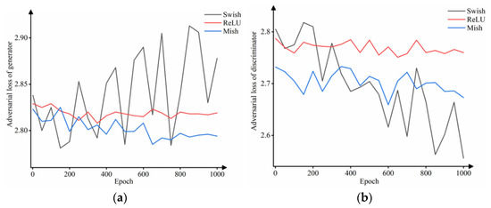
Figure 4.
Using different activation functions to train 1000 epochs: (a) generator adversarial loss curves and (b) discriminator adversarial loss curves.
As shown in Figure 4a, the loss curve of the generator using the Swish function is in a state of oscillation during training, and the loss value does not decrease but shows an upward trend, indicating that the generation quality is reduced and deviates greatly from the real distribution. The generator loss curves using the ReLU and Mish functions show a continuous decline and basically show a stable convergence state after the 800th epoch. However, the generator loss value using the ReLU function decreases slightly, and the convergence state is almost the same as the initial state. The generator loss value using the Mish function is stably reduced and converges to a relatively low value range.
Analysis of the discriminator loss curve in Figure 4b shows that the discriminator using the Swish function is similar to its generator, the whole training process has been oscillating; the discriminator loss curve using the ReLU function has little decreasing trend; and the discriminator using the Mish function shows a steady downward trend overall. Discriminator loss curves using different activation functions all show a downward trend, and there is no sign of convergence, indicating that the performance of the discriminator is better than that of the generator in the training process, which can identify whether the input sequence results are generated by the generator or real results. This phenomenon is due to the traditional GAN model in the data distribution of the distance metric selecting JS divergence. Section 3.1 uses the Wasserstein distance to mitigate the problem.
The loss curve of the model during the training process can portray the training situation to a certain extent. For the prediction task of time series satellite cloud images, model prediction results are ultimately judged by the quality of the generated images. Two sets of samples are selected from the test set for experimental comparison, as shown in Table 2. T−3 to T0 represent the four input times, and T1 to T4 represent the four future times. Swish-GAN, ReLU-GAN, and Mish-GAN correspond to models using three activation functions.
Table 2.
Comparison of prediction results by introducing different activation function models.
Comprehensive analysis of Table 2 and Figure 4 shows that the prediction results of color distortion and serious loss of image details of the Swish-GAN model in the case of generator loss curve oscillation increased over time. Comparing the generator loss curves of the ReLU-GAN model and the Mish-GAN model, the generator loss curve of the ReLU-GAN model has little change in the convergence state and the initial state, the model parameters are updated slowly, and the learning ability is not strong. By introducing a smoother Mish activation function, the Mish-GAN model produces a better gradient flow during the parameter update process, the generator loss curve smoothly drops to the convergence state, and the learning ability of the model is improved. Comparing the prediction results of the two models, the ReLU-GAN model does not directly learn the changes of the upper left cloud cluster in the first set of experiments. Moreover, in the prediction results of the latter two times, the airflow distribution on the left side of the first set of experiments and the middle of the second set of experiments is not obvious. The Mish-GAN model has better accuracy and clearly predicts the presence and growth trend of the upper left cloud cluster in the first set of experiments. Moreover, the Mish-GAN model has a more obvious airflow distribution on the left side of the first set of prediction results and the middle of the second set of prediction results, which can maintain a clearer contour and more complete local detail features as a whole. Therefore, the comparative analysis shows that the Mish-GAN model has the best comprehensive performance, but there are still deficiencies in the long-term and sharpness of the prediction results. In the third section, we will improve the experiment based on the Mish-GAN model.
3. Construction and Analysis of an Improved Prediction GAN Model Based on Time Series Cloud Images Features
3.1. Time Series Cloud Images Prediction GAN Model Improvement Scheme
3.1.1. Using the Wasserstein Distance Instead of JS Divergence
For Figure 4, no matter how the generator loss curve trend changes, the discriminator loss curve continues to decline, and no “adversarial” training is achieved during the training process. The reason is that the original GAN model measures the distance between the real distribution and the generated distribution by JS divergence, and minimizing the adversarial loss of the generator is similar to minimizing the JS divergence between and . The process is based on the assumption that and overlap. However, since the number of samples is much smaller than the real distribution, the probability of overlap between the sample distributions obtained from and is almost negligible. In the case that there is no intersection between and , the use of JS divergence as a metric will lead to the value of JS divergence always being , no matter whether is gradually close to , which eventually leads to the stagnation of generator parameter updates and the inability to generate prediction results that can confuse the discriminator.
Therefore, the Wasserstein distance [25] is used to replace the JS divergence as the distance metric between and , as shown in Figure 5. For JS divergence, the distance between and , and the distance between and are both . Unless the parameters of the generator can be exactly updated to the parameters of in one step during training, the parameters of the generator cannot be gradually updated to and then gradually updated to , the training will stagnate. The advantage of using the Wasserstein distance is that even if and do not overlap or overlap very little, the Wasserstein distance still reflects how close they are. Therefore, for the Wasserstein distance, < < , is better than . can update the parameters to and then gradually update to until the distance between and reaches the minimum.
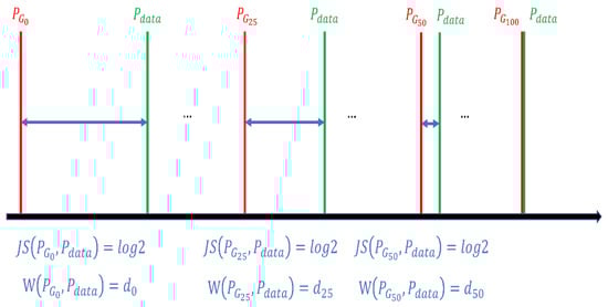
Figure 5.
The difference between the Wasserstein distance and JS divergence as distance measures between distributions.
3.1.2. Using a Multiscale Network Structure
In Section 2, the single-scale prediction GAN model is used. Table 2 shows that over time, the long-term effect of the model prediction is obviously insufficient, and the shape and drift trend of the cloud cluster are still biased from the real results. It is difficult to directly learn the overall sample feature changes through a single-scale model. Therefore, this section cascades different scales of generator and discriminator networks to generate prediction images step by step from small to large. The model structure is shown in Figure 6.
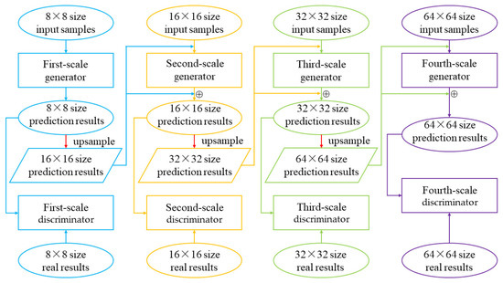
Figure 6.
Structure of the multiscale time series cloud image prediction model.
The first-scale generator downsamples the original input samples to 1/8 size as the starting input and generates prediction results of 1/8 size based on the single-scale generator in Figure 3. At the same time, the prediction results of this size are upsampled to 1/4 the size of the original samples and input into the second-scale generator as a specific condition. The second-scale generator inputs the original samples downsampled to 1/4 size. Under the constraint of specific condition, the residual images are generated, and combined with the prediction results upsampled to 1/4 size, finally the prediction results of 1/4 size are obtained. The discriminator of each scale takes the downsampled version of the prediction images and the real images of the corresponding size as input and performs discriminant output after feature extraction. The multiscale model parameters are shown in Table 3. By capturing the residuals between different scale prediction results step by step, the detailed information, such as cloud cluster texture deformation and movement changes learned by different scale models, is accumulated to simulate the real cloud cluster motion process, which alleviates the problem that the prediction results worsen in cloud cluster shape and movement trend.
Table 3.
Multiscale time series cloud image prediction model parameters.
3.1.3. Introducing Image Gradient Difference Loss
In the prediction results of Table 2, even the Mish-GAN model with the best performance still has the problem of blurred contour edges of cloud clusters and insufficient overall image sharpness. Therefore, this section improves the generator loss function and introduces the image gradient difference loss (GDL) [26]. By considering the difference in adjacent pixel intensity, the gradient difference between the prediction results and real results is penalized. The definition is as follows in Equation (6):
In Equation (6), represents the prediction results, represents the real results, is an integer equal to 1, and represents the absolute value function. Therefore, this section proposes a new generator joint loss function. The specific formula is shown in Equation (7):
In Equation (7), is the weight coefficient of adversarial loss, is the weight coefficient of L1 loss, and is the weight coefficient of GDL.
In the process of using the joint loss function training, the adversarial loss promotes the residual extraction of each scale generator and accurately predicts the high-frequency information such as the birth and disappearance changes and movement trends of cloud images. L1 loss preserves the underlying information of images to ensure the structural consistency of the prediction cloud images in the low frequency part. The image gradient difference loss effectively maintains the global similarity and contour edge detail features of the prediction images and real images through similarity supervision and improves the overall visual effect of the prediction results. The three are optimized from different levels to improve the accuracy, longevity, and visual quality of the prediction results.
3.2. Experiments and Qualitative Analysis
Based on the Mish-GAN model and the above three improvement measures, this section adopts the training mode of Wasserstein GAN and uses the Adam optimizer instead of SGD. The initial learning rate is the same as that of Section 2, and are 0.5 and 0.9, respectively. The weight coefficients , , and of the joint loss function are 1, 0.1, and 0.05, respectively.
The discriminator no longer classifies the prediction results and real results but calculates the Wasserstein distance between the two. Therefore, in the training process, the adversarial loss between the generator and discriminator is no longer calculated by Log, and the final sigmoid function of the discriminator is removed. The loss curves of the improved model (GDL-GAN) training 1000 epochs are shown in Figure 7.
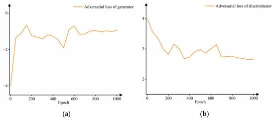
Figure 7.
Improved time series cloud image prediction GAN model based on the Wasserstein distance: (a) generator adversarial loss curve and (b) discriminator adversarial loss curve.
As shown in Figure 7a, the adversarial loss of the generator increases and gradually converges after 700th epochs, indicating that the score of the discriminator obtained by the prediction result is increased to a stable value range. As shown in Figure 7b, the discriminator loss curve continues to decline and finally reaches a convergence state after 700th epochs, which means that the difference between the generated distribution and the real distribution gradually narrows and tends to be stable. Therefore, the Wasserstein distance is used instead of the JS divergence as the metric of the loss function of the prediction model. While ensuring the stability of the model and improving the prediction quality, it enters the convergence state earlier and achieves the goal of “confusing” the discriminator with the prediction results. The problem of nonconvergence of the discriminator loss curve in Figure 4 is improved.
For a more intuitive demonstration of the prediction effect of the improved model (GDL-GAN), this section still selects the same two sets of samples as in Section 2 and compares the Mish-GAN model, as shown in Table 4. We show the prediction results of more sets of experiments in Table A1, Table A2 and Table A3 of Appendix A.
Table 4.
Prediction results of different models.
From the truth of Table 4, it is observed that in the first set of experiments, the spiral air flow rotates counterclockwise, and the cloud image moves slowly eastward as a whole. In the second set of experiments, the banded cloud clusters gradually move eastward, accompanied by partial dissipation. For the Mish-GAN model, the first set of experiments can roughly predict the location of the cyclone, but the last two prediction results are only a U-shaped block lacking the details of air flow rotation and motion trend. In the second set of prediction results, the upper cloud cluster boundary has fuzzy bright spots, and the dissipation characteristics of banded cloud clusters are not obvious. In contrast, the prediction effect of the GDL-GAN model is improved, which is mainly reflected in the following two aspects: (1) not only the evolution law of cyclones and banded cloud clusters in the two sets of prediction results is accurately modeled but also the textural details of the spiral cyclone center structure and the air flow distribution on the west side in the first set of results can be predicted more accurately in the last two times, and the dissipation prediction of the cloud clusters in the second set of results is more accurate. (2) The contour of cloud clusters and airflow edge is clear, which is closer to the real results. The overall sharpness of the prediction cloud images is improved, and the visual effect is better.
3.3. Quantitative Analysis of Time Series Cloud Images Prediction Results
In the previous experimental process, we analyzed the quality of the prediction results through visual interpretation. To accurately measure the prediction performance of the improved model (GDL-GAN), this section continues to use the peak signal-to-noise ratio (PSNR) [27], structural similarity (SSIM) [28], mean absolute error (MAE), and root mean square error (RMSE) four evaluation indicators for quantitative comparison. Among them, MAE and RMSE are pixel-level indicators to calculate the difference between the prediction results and the real results. The smaller the values of MAE and RMSE, the closer the pixel values between the prediction results and the real results. PSNR is a method to estimate the image quality of prediction results based on error sensitivity. SSIM is used to measure the structural similarity between the prediction and real results. It was proposed under the assumption that the quality perception of human visual system (HVS) is correlated with structural information of the scene. The larger the values of PSNR and SSIM, the better the image quality of the prediction results and the higher the similarity with the real results.
Table 5 shows the quantitative performance of the unimproved model using the three activation functions and the improved model on the test set of four evaluation indicators, which are the average of the prediction results at the next four times. Table 5 shows that the GDL-GAN model performs best in four indicators. The GDL-GAN model is higher than the other three models in terms of prediction accuracy and image quality. Compared with Mish-GAN, which has the highest index among the unimproved models, the GDL-GAN model significantly reduces the MAE and RMSE values by 18.84% and 7.60%, respectively; the PSNR and SSIM values also increase by 0.44 and 0.02, respectively.
Table 5.
Quantitative performance of prediction results of different models.
To reflect the differences between different models in more detail, this section also compares the prediction results at each time and plots the change curves of the four evaluation indicators, as shown in Figure 8 and Figure 9. It can be seen intuitively from Figure 8 and Figure 9 that the GDL-GAN model shows the best results and the slowest performance degradation on the evaluation indicators at the next four times. The prediction accuracy and quality at each time have been steadily improved. The maximum improvement of PSNR, SSIM, MAE, and RMSE at a single time is 1.93%, 4.19%, 21.84%, and 8.23%, respectively. This shows that the GDL-GAN model improves the imaging quality of the prediction results while ensuring the dynamic accuracy of the prediction sequence cloud images.
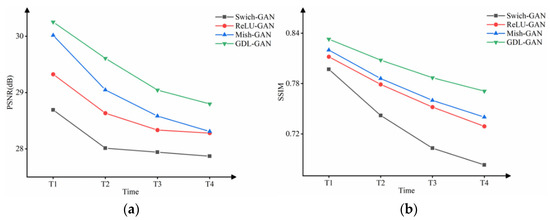
Figure 8.
The change curves of four models in the next four times on (a) PSNR and (b) SSIM indicators.
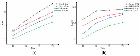
Figure 9.
The change curves of four models in the next four times on (a) MAE and (b) RMSE indicators.
Reference comparison of GDL-GAN model with optical flow model and computer vision model:
Based on the quantitative analysis in this section, the relevant literatures on satellite cloud images prediction are consulted for reference comparison. Su et al. [29] constructed a Multi-GRU-RCN prediction model for FY-2G infrared satellite cloud images based on gated recurrent unit (GRU) and recurrent convolutional network (RCN). The results show that the average PSNR and SSIM of the satellite cloud images at the next time are 29.62 and 0.79, respectively, and the average RMSE is 8.54. The applicability of the model is better than that of deep learning models such as LSTM, GRU and ConvLSTM. Shi et al. [6] extrapolated the FY-4A infrared satellite cloud images by using a dense optical flow model. The average MAE and RMSE of the prediction cloud images at the next four times are below 15.
In terms of the quality of the prediction results, the average PSNR and SSIM of the GDL-GAN model constructed in this paper are 30.25 and 0.83 at the next time. Compared with the Multi-GRU-RCN model, the image quality of the prediction results is enhanced. This improvement is due to the combination of L1 loss, adversarial loss and image gradient difference loss to form a joint loss function to guide model training, which reduces the ambiguity of the prediction results caused by relying solely on L1 loss or L2 loss.
In terms of the accuracy of the prediction cloud images, the average RMSE of the GDL-GAN model in predicting the next time is 7.53, and the average MAE and RMSE of the next four times are 18.05 and 8.39. MAE is slightly inferior to the dense optical flow model, but the accuracy level of MAE is kept in the same range. For the RMSE index, the GDL-GAN model achieves values smaller than the Multi-GRU-RCN model and the dense optical flow model. It shows that the improvement measure of step-by-step prediction through multiscale network structure improves the accuracy and long-term effectiveness of prediction results to a certain extent.
Based on the qualitative and quantitative analysis, three improvement measures have achieved corresponding results. The Wasserstein distance instead of JS divergence avoids the problem that the generator reaches the convergence state before improvement, but the prediction results are still easily distinguished by the discriminator, the overall stable update and convergence of the model are realized. Through the step-by-step prediction of multiscale network structure, the prediction cloud images can always maintain a high degree of similarity with real cloud images in terms of overall motion trend and texture details in the next four times. The generator loss function introduces the image gradient difference loss to jointly guide the generated prediction sequence images to have more obvious image sharpness and visual realism. This section is effective for the improvement of the time series prediction GAN model.
4. Conclusions
In this paper, a time series satellite cloud image prediction model is constructed based on GAN, and satellite cloud image prediction experiments are carried out for the next four times. The loss curves during the training process are analyzed, and the prediction results are qualitatively compared. Among the models using different activation functions, Mish-GAN performs best. On this basis, three improvement measures are proposed for the problems in the GAN model experiment of time series satellite cloud image prediction: Wasserstein distance instead of JS divergence ensures that the parameters can be updated normally during generator training; the multiscale network structure is used to extract and learn the image features at different scales step by step, so that the model can achieve better long-term performance in the prediction results; on the basis of adversarial loss and L1 loss, the image gradient difference loss is combined to obtain better image sharpness performance. According to the three measures, the model is improved, and the experiment and quantitative analysis have been carried out. Compared with the Mish-GAN unimproved model, the improved GDL-GAN model increases the MAE and RMSE by 18.84% and 7.60% on average, and the prediction accuracy at a single time is increased by 21.84% and 8.23% at most. The PSNR and SSIM are improved by 0.44 and 0.02 on average, and the prediction quality at a single time is improved by 1.93% and 4.19% at most. The experimental results prove the effectiveness of the improved scheme. The time series satellite cloud image prediction GAN model constructed in this paper can significantly improve the visualization effect of the prediction sequence cloud images and the accuracy of the overall motion trend.
Author Contributions
Data curation, D.T. and W.Y.; funding acquisition, R.W. and X.Z.; methodology, R.W. and J.Z.; software, D.T.; writing—original draft, D.T. and R.W.; writing—review and editing, R.W., X.Z. and J.Z. All authors have read and agreed to the published version of the manuscript.
Funding
This research was funded by the Natural Science Foundation of Shandong Province (Grant Nos. ZR2022MD002); the Marine Project (2205cxzx040431); the Key Laboratory of marine surveying and mapping, Ministry of natural resources (2021B06).
Data Availability Statement
Not applicable.
Conflicts of Interest
The authors declare no conflict of interest.
Appendix A
We show more prediction results on the test set in Table A1, Table A2 and Table A3. Based on the analysis of the eight sets of experiments in Table 4, Table A1, Table A2 and Table A3, the first six sets of experiments show better and more stable results, and the motion trend in the prediction cloud images is basically consistent with the real situation. For example, the evolution trend of the strengthening, dissipation, and maintenance of spiral weather phenomena in the first, third and fifth sets of experiments is consistent with the real motion trend; in the second, fourth, and sixth sets of experiments, the spatial variation features such as cloud clusters formation and dissipation and drift motion are accurately predicted. In addition, in the first six sets of experiments, the GDL-GAN model reflects the brightness temperature more realistically. Compared with the Mish-GAN model, the GDL-GAN model reduces the ambiguity of the prediction results and the cloud cluster boundary is clear and discernible.
However, the GDL-GAN model still has shortcomings. In the seventh and eighth sets of experiments, although the motion trend of the prediction cloud images is well predicted, the response is not sensitive enough for the change of brightness temperature. For example, in the lower right corner of the seventh set of experiments and the lower half of the eighth set of experiments, the brightness temperature predicted by the GDL-GAN model is lower than the real results for the area with high and dense brightness temperature, the long-term effectiveness of the model prediction results needs to be further improved.
Table A1.
The prediction results of the third and fourth sets of experiments.
Table A1.
The prediction results of the third and fourth sets of experiments.
| The Third Set of Experiments | The Fourth Set of Experiments | |||||||
|---|---|---|---|---|---|---|---|---|
| Input sequence samples | Input sequence samples | |||||||
 |  |  |  |  |  |  |  | |
| T−3 | T−2 | T−1 | T0 | T−3 | T−2 | T−1 | T0 | |
| prediction results | prediction results | |||||||
 |  |  |  | Mish-GAN |  |  |  |  |
 |  |  |  | GDL-GAN |  |  |  |  |
| T1 | T2 | T3 | T4 | T1 | T2 | T3 | T4 | |
| real results | real results | |||||||
 |  |  |  |  |  |  |  | |
| T1 | T2 | T3 | T4 | T1 | T2 | T3 | T4 | |
Table A2.
The prediction results of the fifth and sixth sets of experiments.
Table A2.
The prediction results of the fifth and sixth sets of experiments.
| The Fifth Set of Experiments | The Sixth Set of Experiments | |||||||
|---|---|---|---|---|---|---|---|---|
| Input sequence samples | Input sequence samples | |||||||
 |  |  |  |  |  |  |  | |
| T−3 | T−2 | T−1 | T0 | T−3 | T−2 | T−1 | T0 | |
| prediction results | prediction results | |||||||
 |  |  |  | Mish-GAN |  |  |  |  |
 |  |  |  | GDL-GAN |  |  |  |  |
| T1 | T2 | T3 | T4 | T1 | T2 | T3 | T4 | |
| real results | real results | |||||||
 |  |  |  |  |  |  |  | |
| T1 | T2 | T3 | T4 | T1 | T2 | T3 | T4 | |
Table A3.
The prediction results of the seventh and eighth sets of experiments.
Table A3.
The prediction results of the seventh and eighth sets of experiments.
| The Seventh Set of Experiments | The Eighth Set of Experiments | |||||||
|---|---|---|---|---|---|---|---|---|
| Input sequence samples | Input sequence samples | |||||||
 |  |  |  |  |  |  |  | |
| T−3 | T−2 | T−1 | T0 | T−3 | T−2 | T−1 | T0 | |
| prediction results | prediction results | |||||||
 |  |  |  | Mish-GAN |  |  |  |  |
 |  |  |  | GDL-GAN |  |  |  |  |
| T1 | T2 | T3 | T4 | T1 | T2 | T3 | T4 | |
| real results | real results | |||||||
 |  |  |  |  |  |  |  | |
| T1 | T2 | T3 | T4 | T1 | T2 | T3 | T4 | |
References
- Norris, J.R.; Allen, R.J.; Evan, A.T.; Zelinka, M.D.; O’Dell, C.W.; Klein, S.A. Evidence for climate change in the satellite cloud record. Nature 2016, 536, 72–75. [Google Scholar] [CrossRef] [PubMed]
- Lu, N.; Zheng, W.; Wang, X.; Gao, L.; Liu, Q.; Wu, S.; Jiang, J.; Gu, S.; Fang, X. Overview of Meteorological Satellite and Its Data Application in Weather Analysis, Climate and Environment Disaster Monitoring. J. Mar. Meteorol. 2017, 37, 20–30. [Google Scholar] [CrossRef]
- Filonchyk, M.; Hurynovich, V. Validation of MODIS Aerosol Products with AERONET Measurements of Different Land Cover Types in Areas over Eastern Europe and China. J. Geovisual. Spat. Anal. 2020, 4, 10. [Google Scholar] [CrossRef]
- Zinner, T.; Mannstein, H.; Tafferner, A. Cb-TRAM: Tracking and monitoring severe convection from onset over rapid development to mature phase using multi-channel Meteosat-8 SEVIRI data. Meteorol. Atmos. Phys. 2008, 101, 191–210. [Google Scholar] [CrossRef]
- Jamaly, M.; Kleissl, J. Robust cloud motion estimation by spatio-temporal correlation analysis of irradiance data. Sol. Energy 2018, 159, 306–317. [Google Scholar] [CrossRef]
- Shi, Y.; Shi, S. Research on Accuracy Evaluation of Optical Flow Algorithm in FY-4A Infrared Image Extrapolation. J. Ordnance Equip. Eng. 2021, 42, 150–158+224. [Google Scholar]
- Dissawa, D.M.L.H.; Ekanayake, M.P.B.; Godaliyadda, G.M.R.I.; Ekanayake, J.B.; Agalgaonkar, A.P. Cloud motion tracking for short-term on-site cloud coverage prediction. In Proceedings of the Seventeenth International Conference on Advances in ICT for Emerging Regions (ICTer), Colombo, Sri Lanka, 6–9 September 2017; pp. 1–6. [Google Scholar]
- Liang, L.; Yang, X.; Yin, J.; Hu, G.; Ren, F. The New Short-Term Cloud Forecast Method. Plateau Meteorol. 2015, 34, 1186–1190. [Google Scholar]
- Pang, S. Research on Minute-Mevel Cloud Displacement Prediction Model Based on Motion Pattern Recognition; School of Electrical and Electronic Engineering: Penang, Malaysia, 2019. [Google Scholar]
- Wang, W.; Liu, J.; Meng, Z. ldentifying and Tracking Convective Clouds Based on Time Series Remote Sensing Satellite Images. Acta Electron. Sin. 2014, 42, 804–808. [Google Scholar]
- Du, P.; Bai, X.; Tan, K.; Xue, Z.; Samat, A.; Xia, J.; Li, E.; Su, H.; Liu, W. Advances of Four Machine Learning Methods for Spatial Data Handling: A Review. J. Geovisual. Spat. Anal. 2020, 4, 13. [Google Scholar] [CrossRef]
- He, R.; Guan, Z.; Jin, L. A Short-term Cloud Forecast Model by Neural Networks. Trans. Atmos. Sci. 2010, 33, 725–730. [Google Scholar] [CrossRef]
- Jin, L.; Huang, Y.; He, R. Nonlinear ensemble prediction model for satellite image based on genetic neural network. Comput. Eng. Appl. 2011, 47, 231–235+248. [Google Scholar]
- Penteliuc, M.; Frincu, M. Prediction of Cloud Movement from Satellite Images Using Neural Networks. In Proceedings of the 2019 21st International Symposium on Symbolic and Numeric Algorithms for Scientific Computing (SYNASC), Timisoara, Romania, 4–7 September 2019; pp. 222–229. [Google Scholar]
- Huang, X.; He, L.; Zhao, H.; Huang, Y.; Wu, Y. Application of Shapley-fuzzy neural network method in long-time rolling forecasting of typhoon satellite image in South China. Acta Meteorol. Sin. 2021, 79, 309–327. [Google Scholar]
- Goodfellow, I.J.; Pouget-Abadie, J.; Mirza, M.; Xu, B.; Warde-Farley, D.; Ozair, S.; Courville, A.; Bengio, Y. Generative adversarial nets. In Proceedings of the Neural Information Processing Systems, Montreal, QC, Canada, 8–13 December 2014; pp. 2672–2680. [Google Scholar]
- Awiszus, M.; Schubert, F.; Rosenhahn, B. Toad-gan: Coherent style level generation from a single example. In Proceedings of the AAAI Conference on Artificial Intelligence and Interactive Digital Entertainment, Virtual, 19–23 October 2020; pp. 10–16. [Google Scholar]
- Nguyen, K.-T.; Dinh, D.-T.; Do, M.N.; Tran, M.-T. Anomaly detection in traffic surveillance videos with gan-based future frame prediction. In Proceedings of the 2020 International Conference on Multimedia Retrieval, Dublin, Ireland, 8–11 June 2020; pp. 457–463. [Google Scholar]
- Yan, Y.; Xu, J.; Ni, B.; Zhang, W.; Yang, X. Skeleton-Aided Articulated Motion Generation. In Proceedings of the 25th ACM International Conference on Multimedia, Mountain View, CA, USA, 23–27 October 2017; pp. 199–207. [Google Scholar]
- Xu, Z.; Du, J.; Wang, J.; Jiang, C.; Ren, Y. Satellite Image Prediction Relying on GAN and LSTM Neural Networks. In Proceedings of the ICC 2019—2019 IEEE International Conference on Communications (ICC), Shanghai, China, 20–24 May 2019; pp. 1–6. [Google Scholar]
- Isola, P.; Zhu, J.Y.; Zhou, T.; Efros, A.A. Image-to-Image Translation with Conditional Adversarial Networks. In Proceedings of the 2017 IEEE Conference on Computer Vision and Pattern Recognition (CVPR), Honolulu, HI, USA, 21–26 July 2017; pp. 5967–5976. [Google Scholar]
- Heusel, M.; Ramsauer, H.; Unterthiner, T.; Nessler, B.; Hochreiter, S. Gans trained by a two time-scale update rule converge to a local nash equilibrium. Adv. Neural Inf. Process. Syst. 2017, 30. Available online: https://proceedings.neurips.cc/paper/2017/hash/8a1d694707eb0fefe65871369074926d-Abstract.html (accessed on 6 September 2022).
- Ramachandran, P.; Zoph, B.; Le, Q. Searching for activation functions. arXiv 2017, arXiv:1710.05941. [Google Scholar]
- Misra, D. Mish: A self regularized non-monotonic neural activation function. arXiv 2019, arXiv:1908.08681. [Google Scholar]
- Arjovsky, M.; Chintala, S.; Bottou, L. Wasserstein GAN. arXiv 2017, arXiv:1701.07875. [Google Scholar]
- Mathieu, M.; Couprie, C.; LeCun, Y. Deep multi-scale video prediction beyond mean square error. arXiv 2015, arXiv:1511.05440. [Google Scholar]
- Cuevas, E.; Zaldívar, D.; Pérez-Cisneros, M.; Oliva, D. Block-matching algorithm based on differential evolution for motion estimation. Eng. Appl. Artif. Intell. 2013, 26, 488–498. [Google Scholar] [CrossRef]
- Zhou, W.; Bovik, A.C.; Sheikh, H.R.; Simoncelli, E.P. Image quality assessment: From error visibility to structural similarity. IEEE Trans. Image Process. 2004, 13, 600–612. [Google Scholar] [CrossRef]
- Su, X.; Li, T.; An, C.; Wang, G. Prediction of Short-Time Cloud Motion Using a Deep-Learning Model. Atmosphere 2020, 11, 1151. [Google Scholar] [CrossRef]


Publisher’s Note: MDPI stays neutral with regard to jurisdictional claims in published maps and institutional affiliations. |
© 2022 by the authors. Licensee MDPI, Basel, Switzerland. This article is an open access article distributed under the terms and conditions of the Creative Commons Attribution (CC BY) license (https://creativecommons.org/licenses/by/4.0/).