Abstract
Rapid extraction of liquefaction induced by strong earthquakes is helpful for earthquake intensity assessment and earthquake emergency response. Supervised classification methods are potentially more accurate and do not need pre-earthquake images. However, the current supervised classification methods depend on the precisely delineated polygons of liquefaction by manual and landcover maps. To overcome these shortcomings, this study proposed two binary classification methods (i.e., random forest and gradient boosting decision tree) based on typical samples. The proposed methods trained the two machine learning methods with different numbers of typical samples, then used the trained binary classification methods to extract the spatial distribution of liquefaction. Finally, a morphological transformation method was used for the postprocessing of the extracted liquefaction. The recognition accuracies of liquefaction were estimated by four evaluation indices, which all showed a score of about 90%. The spatial distribution of liquefaction pits is also consistent with the formation principle of liquefaction. This study demonstrates that the proposed binary classification methods based on machine learning could efficiently and quickly provide the spatial distribution of liquefaction based on post-earthquake emergency satellite images.
1. Introduction
Coseismic liquefaction refers to the change of sand from a solid state to a liquid state caused by rising pore water pressure and decreasing effective stress when an earthquake occurs [1,2,3]. As relevant to coseismic surface rupture, rapid acquisition of the spatial distribution of liquefaction is helpful for earthquake intensity assessment and earthquake emergency response [4,5]. In addition, post-earthquake investigation of liquefaction is a fundamental way of developing knowledge on seismic engineering and provides the basis for seismic-resistant design theories [6,7]. A complete liquefaction investigation could also help enrich the globe case base of liquefaction induced by the earthquake.
Currently, the identification of liquefaction usually depends on the field investigation, which can be time-consuming and labor-intensive. More importantly, due to lack of accessibility, this method could not obtain the complete spatial distribution of liquefaction, especially in highland areas. Thus, developing automatic extraction methods based on satellite or aerial images could be helpful in overcoming the shortcomings of field investigation.
The existing automatic identification of liquefaction can be summarized into two groups. The first group is the unsupervised classification strategy, which does not need liquefaction samples. This strategy detects liquefaction by comparing pre- and post-earthquake images [2,8,9,10]. For example, Ishitsuka et al. [11] identified the extent of liquefaction induced by the 2011 Tohoku earthquake by analyzing the surface changes with pre- and post-synthetic aperture radar (SAR) images. Baik et al. [12] detected liquefaction by identifying the areas where sudden water content increases occurred with SAR and optical satellite images. Those methods obtained liquefaction automatically without liquefaction samples. However, the performance of these methods often depends on the quality of the images. The quality of the images was usually influenced by the imaging time, weather, resolution and so on. Furthermore, those methods usually fail when the pre-earthquake images close to the time of the earthquake do not exist.
The second group is the supervised classification strategy based on post-earthquake images. The supervised classification strategy needs to collect a certain number of samples of liquefaction pits in advance [13,14]. This strategy could be further divided into pixel-based and object-based methods. The pixel-based methods focus on the spectral characteristic of liquefaction pits in each pixel rather than considering the morphological features of liquefaction. For example, Rashidian et al. [15] used the maximum likelihood classifier to map the spatial distribution of liquefaction pits triggered by the 2011 Christchurch earthquake based on satellite and aerial images. Object-based methods integrate similar pixels into a liquefaction object and distinguish the liquefaction objects from other landcover objects by morphological features. Morgenroth et al. [16] used object-based methods to extract the liquefaction pits induced by the 2011 Christchurch earthquake with aerial photography, light detection and ranging images. These methods avoid using pre-earthquake images, and usually have more accurate and robust identification results than unsupervised methods.
Due to the morphological features (e.g., size, shape) of liquefaction pits, object-based methods usually require very high-resolution images, such as unmanned aerial vehicle (UAV) images. Compared to UAV images, the satellite-based images have a lower resolution, which makes it difficult to recognize the morphology of liquefaction pits [17,18]. However, satellite-based images are the easier-to-access images and cover a large area. These images are the most-used in an earthquake emergency. Thus, it is necessary to develop pixel-based methods for satellite-based images.
Currently, pixel-based methods always need the user to collect landcover maps to assist in selecting non-liquefaction/liquefaction samples [15]. Nevertheless, high-resolution landcover maps are hard to obtain, and the available classes of landcover maps are not used for recognizing liquefaction pits. Meanwhile, the current supervised methods need users to draw polygons of liquefaction very carefully. The boundary of liquefaction is usually so vague that they are difficult to draw. The wrong points may lead to a decrease in identification accuracy [19].
To solve the above problems, this paper proposed a binary supervised classification framework. The binary classification framework does not require the assistance of a landcover map, and users can focus on selecting typical pixel samples for non-liquefaction/liquefaction as training samples. This framework can help recognize liquefaction pits based on satellite-based images in a short time. The binary classification framework was implemented with random forest (RF) and gradient boosting decision tree (GBDT). RF and GBDT handled high-dimensional data and select covariates. These advantages helped the expansion of the sample base and the addition of new covariates.
2. Materials and Methods
2.1. Study Area
The proposed method was examined in the coseismic liquefaction induced by the 22 May 2021, Mw 7.3 Maduo on the Tibetan Plateau, Western China. The seismogenic fault of the Maduo earthquake is an active NW-striking and left–lateral strike-slip fault with lower slip rate. The length of coseismic surface rupture is approximately 160 km with massive liquefaction pits in river valleys and swampy areas around the source area of the Yellow River [20].
The investigated area is approximately 45 km2 and located near the Yematan site, 30 km west of the epicenter, ranging from 97.9°E to 98.02°E longitude and 34.64°N to 34.74°N latitude (Figure 1). The elevation of this study ranges between 4190 m and 4512 m and has a gentle gradient with a mean slope gradient under 10°.
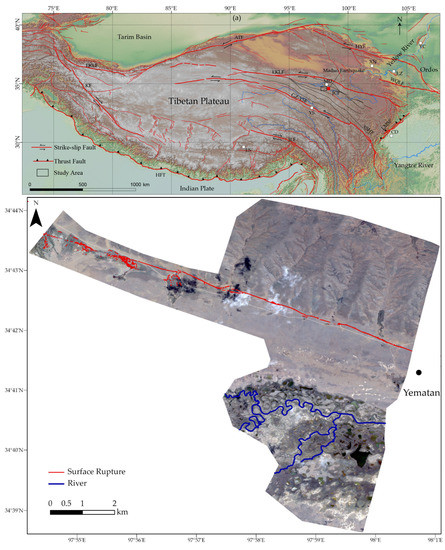
Figure 1.
The location and remote sensing images of the study area. (a) The tectonic environment around the study area, (b) the GF-7 satellite image of the study area the surface rupture data came from [20]. EKLF, Eastern Kunlun Fault; GZ-YSF, Ganzi–Yushu Fault; XSHF, Xianshuihe Fault; LMSF, Longmenshan Fault; WQLF, Western Qinling Fault; JLF, Jiali Fault; JCF, Jiangcuo fault; HYF, Haiyuan Fault; ATF, Altyn Falut; KF, Kunlun Fault; HFT, Himalayan Thrust Fault; SF, Sagaing Fault; MD, Maduo; CD, Chengdu; YC, Yinchuan; LZ, Lanzhou; LS, Lhasa; XN, Xining.
2.2. Data Sources
2.2.1. Satellite Images and Derived Covariates
In this study, Gaofen-7 (GF-7) images were collected for identifying the coseismic liquefaction. GF-7 is a stereo mapping satellite launched by China in 2019. It can effectively acquire panchromatic stereo images and multi-spectral images. The backward and forward panchromatic images have a width of 20 km and the resolution is greater than 0.8 m. Multi-spectral imaging features four spectral bands (blue, green, red and near infrared) with a resolution of 3.2 m (Table 1). In this study, a stereo pair of GF-7 images with a few clouds was captured on 10 June 2021, 19 days after the earthquake (Figure 1b).

Table 1.
The images used in this study and the band parameters.
Besides the GF-7 image, another two kinds of image were used for validation in this study. Firstly, a Gaofen-1D image (GF-1D) that was captured on 29 April 2021, was used as the pre-earthquake image (Table 1). Meanwhile, the collected GF-1D image covered the whole study area.
The second were the UAV images captured on 25 July 2021, with a resolution of 0.1 m. The aim of the UAV images was to capture the surface rupture zone of the Maduo earthquake, and the images were mainly located in the north of the study area.
Before using the satellite images, two main methods of processing the GF-7 and GF-1D were applied. The first was pan-sharpening, in which the backward panchromatic image and multi-spectral image were fused into a new image with a 0.8 m resolution. Therefore, multi-spectral images could benefit from the high spatial resolution of panchromatic stereo images. The second process was to generate a 0.8 m resolution of the digital surface model (DSM) by using the forward-and-backward panchromatic images.
Based on the processed GF-7 data, three types of covariates were derived for identifying liquefaction:
- Terrain parameters: We used elevation, slope, all derived at 0.8 m resolution. Since liquefaction often occurs in flat and swampy areas, terrain parameters are mainly used to characterize topographic features.
- Spectral bands: Blue (B), Green (G), Red (R), Near infrared (NIR) of GF-7 were all included.
- Spectral indices: Five spectral indices include, Normalized difference water index (NDWI), Normalized difference vegetation index (NDVI), Modified soil vegetation adjusted index (MSAVI2), Salinity index (Salinity), Grain size index (GSI).
NDWI is an important spectral index for measuring water in vegetation and detecting open water [21]. It has also been used for identifying liquefaction by Sengar et al. [22] and baik et al. [12].
Although NDVI is one of the important parameters for reflecting crop growth and nutritional information, it can also reflect the background influence of plant canopy, such as soil, wet ground, snow, dead leaves and roughness [23]. Thus, in addition to vegetation classification, NDVI is also widely used in the classification of other land features, such liquefaction [10,22].
MSAVI2 is also a kind of vegetation index, which was developed to minimize soil influence using a self-adjustment factor [24].
Salinity combines the R and NIR bands to detect the surface reflectance of salt-affected land [25].
GSI uses three types of visible spectral band to reflect the content of silt–clay and fine-sand of topsoil [26].
2.2.2. Liquefaction Samples
A total of 900 samples were collected in this study area, including 300 liquefaction samples and 600 non-liquefaction samples (Figure 2). All the liquefaction samples were located inside the obvious liquefaction pits, not close to the edge as far as possible. Thus, the samples derived could be more representative. The 600 non-liquefaction samples were located in different landscapes including grassland, river/laker, floodplain, road, exposed rock, and so on.
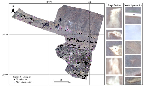
Figure 2.
The spatial distribution of samples and some location details of the non-liquefaction/liquefaction samples.
2.3. Methods
In this study, two ensemble machine learning methods (i.e., RF, GBDT) were used. The principle of ensemble methods is to combine the results of a certain number of estimators to improve robustness. According to the synthesis strategies for the results of different estimators, the ensemble methods could be further distinguished into two classes: averaging methods and boosting methods.
As a typical averaging method, random forest uses multiple decision trees for predicting the classes independently, then uses a majority vote to predict the final result [27]. For a binary classification of liquefaction in this study, each decision tree in the forest would individually determine whether a pixel was liquefaction or not, then RF chose the class with the most votes as the final class. The most important parameters that influence the performance of RF is the number of decision trees (Ntree) and the number of covariates selected for best split (Mtry).
By contrast, the basic idea of a boosting method is to sort the decision trees sequentially; each decision tree will give higher weight to the samples misclassified by previous decision trees during the training process. The final result is obtained by weighting the results of each decision tree. GBDT is a famous boosting method, which was developed by Friedman in 2001 [28]. The most import parameters influencing the performance of GBDT also include Ntree and Mtry. In this study, both parameters were set at default.
The main differences between RF and GBDT can be summarized into two aspects. The first is the sampling strategy; each tree in RF is built by a subset of samples drawn randomly with replacement from the complete sample set. It means the training set of each tree in RF is independent. However, trees in GBDT select subsets of samples from the complete set of samples randomly without replacement. The second different aspect is the classification result. RFs determine the class of each pixel by the majority-vote of all the trees in the RF, while GBDTs integrate the result of each tree using a weighted average method.
Morphological transformations are binary image operations based on the image shape [29]. The transformations usually include two inputs, the original image and the kernel that decides the nature of operation. In this study, the closing operation was selected to fill the gap of the extracted liquefaction.
The complete workflow of extracting liquefaction pits is shown in Figure 3.
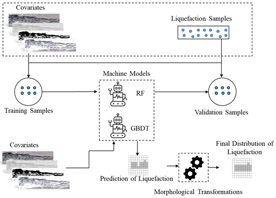
Figure 3.
Flowchart of identifying the liquefaction in this study.
2.4. Cross-Validation and the Evaluation Indices
To evaluate the performance of the proposed methods and the influences of the number of samples, the samples were randomly divided into 20 groups, then choosing 1, 2, 3, …, 19 group/groups as training samples in turn, the rest were used as validation samples. The above processes were repeated 20 times.
For each validation, four quantitative evaluation indices (i.e., Recall, Precision, F1, Kappa) were used to evaluate the performance of the proposed method.
True positives (TP) represent the count of validation samples that were correctly classified into liquefaction by the proposed method. The false positives (FP) are the number of liquefaction samples that were misclassified into non-liquefaction. False negatives (FN) represent the count of non-liquefaction samples that were misclassified into liquefaction. True negatives (TN) are the number of non-liquefaction samples that were correctly classified into non-liquefaction. N represents the number of validation samples.
3. Results
3.1. The Performance of the Two Proposed Methods
The relationship between the evaluation indices of the two classification methods and the number of samples is illustrated in Figure 4. The value of the Kappa index for the RF and GBDT ranged from 0.9 to 0.98 and from 0.87 to 0.97, respectively. The overall accuracies for RF and GBDT ranged from 0.954 to 0.99 and from 0.94 to 0.99, respectively. As for the Recall score, RF ranged from 0.956 to 0.98, a slight rise of 2.5%. However, GBDT had a score lower than 0.9 with the least number of training samples. Like the Kappa indices and overall accuracies, RF and GBDT had similar scores and the same trend in Precision scores. To sum up, RF and GBDT had similar scores in all four indices with the same training samples.
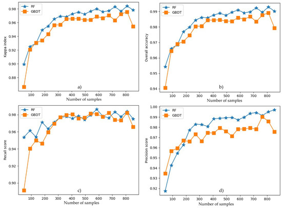
Figure 4.
The relationships between the performance of the two classification methods and the number of samples: (a) relationship between the Kappa index and the increase of the samples; (b) relationship between the overall accuracy and the increase of the samples; (c) relationship between the recall score and the increase of the samples; (d) relationship between the precision score and the increase of the samples.
In addition, the number of samples could have had an influence on the final performance of the classification methods (Figure 4). The four evaluation indices of both classification methods increased when more samples were used as training samples. Compared with RF, GBDT could be more sensitive to the number of training samples when there were a limited number of training samples. Taking the Kappa index as an example, when the number of training samples increased from 45 to 90, the scores increased from 0.87 to 0.92, a rise of 4.6%. However, when the samples reached a certain number, the relationship between the performance of the two proposed methods and the number of training samples was not obvious.
3.2. The Final Prediction of Liquefaction by the Two Proposed Methods
Figure 5 and Figure 6 represent the final distribution of liquefaction that were predicted by the RF and GBDT when there were 270 training samples. Clearly, most of the liquefaction induced by the earthquake located in the southern river valley, Heihe River. Almost no liquefaction was distributed in the northern mountains. The spatial distribution was consistent with the formation principle of liquefaction. The soil in the valleys tends to have a lot of moisture, while the mountain region is often dry and short of groundwater. When an earthquake occurred, the increase of pore water pressure and decrease of effective stress had a greater possibility of occurring in the valley. Therefore, liquefaction pits were usually distributed in the river valley region.
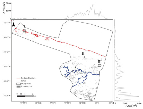
Figure 5.
The distribution of liquefaction predicted by RF when the number of training samples was 270; the surface rupture data came from [20].
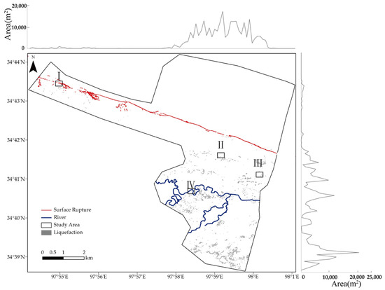
Figure 6.
The distribution of liquefaction predicted by GBDT when the number of training samples was 270; the surface rupture data came from [20].
Figure 7, Figure 8, Figure 9 and Figure 10 show the details of liquefaction (region I, II, III, IV in Figure 5 and Figure 6) identified by the RF and GBDT. For region I, three types of images (i.e., GF-1D, GF-7 and UAV) are available. Compared to the pre-earthquake images (GF-1D), the post-earthquake images (GF-7) show clear surface change, and RF and GBDT identified those places as liquefaction-induced by the earthquake. In the UAV, the morphological characteristics of liquefaction were very obvious, while the size of the liquefaction in the UAV image was smaller than the liquefaction identified with GF-7 images by RF and GBDT. One possible reason is that GF-7 images have lower resolution than UAV images, and the discrete liquefaction could be grouped together in satellite images with low resolution.
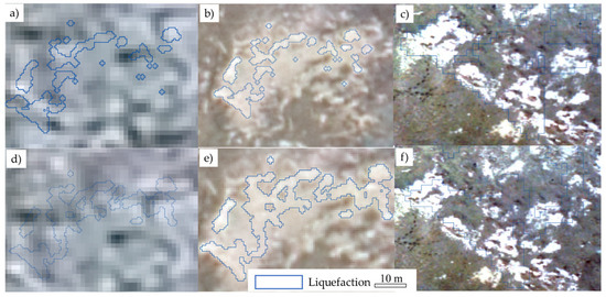
Figure 7.
The extracted liquefaction (region I) by the two proposed methods. (a) GF-1D image pre-earthquake with liquefaction extracted by RF. (b) GF-7 image post-earthquake with the liquefaction predicted by RF. (c) UAV image post-earthquake with liquefaction predicted by RF. (d) GF-1D image pre-earthquake with liquefaction predicted by GBDT. (e) GF-7 image post-earthquake with liquefaction predicted by GBDT. (f) UAV image post-earthquake with liquefaction predicted by GBDT.
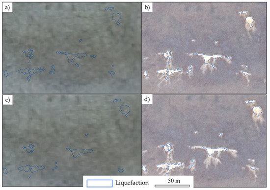
Figure 8.
The extracted liquefaction (region II) by the two proposed methods. (a) GF-1D images pre-earthquake with liquefaction predicted by RF. (b) GF-7 images post-earthquake with liquefaction predicted by RF. (c) GF-1D images pre-earthquake with liquefaction predicted by GBDT. (d) GF-7 images post-earthquake with the liquefaction predicted by GBDT.
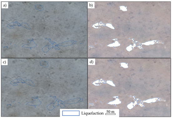
Figure 9.
The extracted liquefaction (region III) by the two proposed methods. (a) GF-1D image pre-earthquake with liquefaction predicted by RF. (b) GF-7 image post-earthquake with liquefaction predicted by RF. (c) GF-1D image pre-earthquake with liquefaction predicted by GBDT. (d) GF-7 image post-earthquake with liquefaction predicted by GBDT.
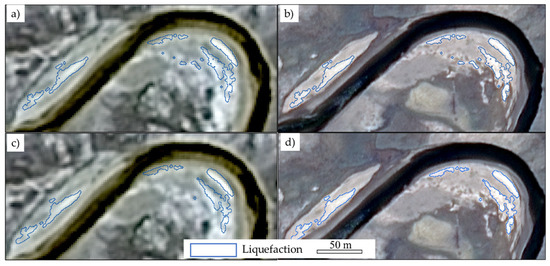
Figure 10.
The extracted liquefaction (region IV) by the two proposed methods. (a) GF-1D image pre-earthquake with liquefaction predicted by RF. (b) GF-7 image post-earthquake with liquefaction predicted by RF. (c) GF-1D image pre-earthquake with liquefaction predicted by GBDT. (d) GF-7 image post-earthquake with liquefaction predicted by GBDT.
Similar to the images in region I, the images pre- and post-earthquake in region II and region III also showed differences and were extracted by RF and GBDT as liquefaction-induced (Figure 8 and Figure 9). However, the shape and size of liquefaction predicted by RF and GBDT were more similar in region III. This is because the boundaries of liquefaction were clearly distinguished from the surrounding ground features in region III. In that satiation, RF and GBDT could effectively identify the liquefaction based on a small number of liquefaction samples. However, when the boundary was relatively fuzzy, neither of the two proposed methods could completely identify the liquefaction morphology of the liquefaction (Figure 7 and Figure 8). The incomplete identification of liquefaction could lead to the difference in area and quantity of liquefaction. Taking the liquefaction located in Figure 8 as an example, complete liquefaction could be divided into a number of small parts and affect the number and area of identified liquefaction.
In region IV, compared to the pre-earthquake image, the post-earthquake image did not show obvious change. However, RF and GBDT both identified some beaches with bare sand as liquefaction-induced. In general, the provenance of the beach around the rivers is close to that of the liquefaction, which is composed of sand. It turned out to be difficult to distinguish the liquefaction from the beach with bare sand.
4. Discussion
4.1. The Area Statistics of the Identified Liquefaction Pits by the Two Proposed Methods
As data-driven methods, RF and GBDT usually predict different spatial distributions of liquefaction with different training samples. Figure 11 and Figure 12 represent the area statistics of the extracted liquefaction with different training samples by RF and GBDT. Clearly, even if the same number of training samples was used, the final area of liquefaction was different, especially when there were a smaller set of training samples. This is because data-driven methods depend heavily on the number and representativeness of training samples [14,19]. Due to the randomly selected training samples in this study, the number and representativeness could be different for each set, especially the training samples of other landcovers that were close to the spectrum of liquefaction. Rashidian et al. [15] designed training liquefaction samples by considering the local classes of landcovers, and keeping the number of training samples representing different landcovers inconsistent. Compared to the multi-class classification method proposed by Rashidian, binary classification methods demand fewer training samples [30]. Thus, in binary classification, the selected training samples should focus on the liquefaction and landcovers that have similar spectral characteristics with liquefaction.
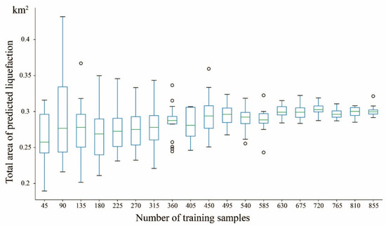
Figure 11.
The relationship between the total area of extracted liquefaction by RF and the number of training samples.
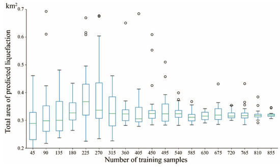
Figure 12.
The relationship between the total area of extracted liquefaction by GBDT and the number of training samples.
4.2. The Importance of Covariates Ranked by RF and GBDT
Successfully selecting and ranking covariates in prediction is one of the greatest abilities of ensemble classifiers such as RF and GBDT, which were used in this study [27,31]. The importance of covariates scored by RF and GBDT were illustrated in Figure 13 and Figure 14, respectively. When different training samples were selected, but the number of samples was the same, the importance of covariates was different (Figure 13b–d and Figure 14b–d). Compared to GBDT, the RF had a relatively small change in the rank of importance of covariates. When the number of training samples used in RF and GBDT increased, the rank of importance of covariates did not show an obvious difference. Meanwhile, the six most important covariates ranked by RF and GBDT were B1, B2, B3, B4, DEM and GSI (Figure 15). The other covariates did not play a significant role in liquefaction classification. The result indicates the consistency of covariate rankings between RF and GBDT. In addition, this also reflects that the selected samples in this study are representative.
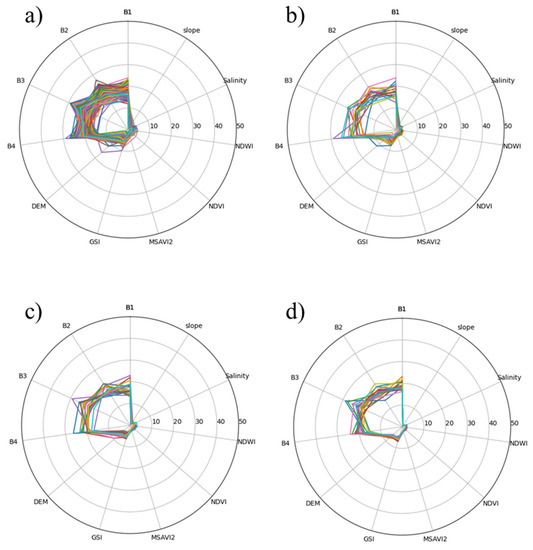
Figure 13.
The relative importance of covariates ranked by RF to extract liquefaction. (a) The importance of covariates in all 380 repeated experiments with different sets of training samples. (b) The statistics of the importance of covariates in 20 repeated experiments when the number of training samples is 90. (c) The statistics of the importance of covariates in 20 repeated experiments when the number of training samples is 270. (d) The statistics of the importance of covariates in 20 repeated experiments when the number of training samples is 630.
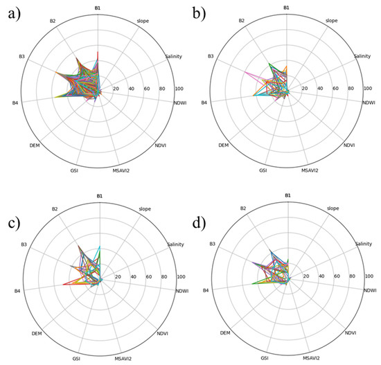
Figure 14.
The relative importance of covariates ranked by GBDT to extract liquefaction. (a) The statistics of the importance of covariates in all 380 repeated experiments with different sets of training samples. (b) The statistics of the importance of covariates in 20 repeated experiments when the number of training samples is 90. (c) The statistics of the importance of covariates in 20 repeated experiments when the number of training samples is 270. (d) The statistics of the importance of covariates in 20 repeated experiments when the number of training samples is 630.
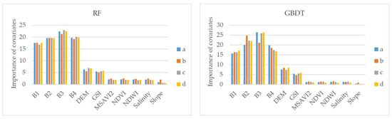
Figure 15.
The mean value of covariates importance ranked by RF and GBDT. (a) Represents the mean statistic of the importance of covariates in all 380 repeated experiments with different sets of training samples. (b) Represents the mean statistic of the importance of covariates in 20 repeated experiments when the number of training samples is 90. (c) Represents the mean statistic of the importance of covariates in 20 repeated experiments when the number of training samples is 270. (d) Represents the mean statistic of the importance of covariates in 20 repeated experiments when the number of training samples is 630.
4.3. The Spatial Distribution of the Liquefaction Pits
According to the previous report, the liquefaction pits were observed during several earthquakes, such as the 1964 M 9.2 Alaska [32], 1999 7.5 Chi-Chi earthquakes [33], 2008 M 8 Wenchuan earthquake [6,7], 2011 M6.2 Christchurch earthquake [15]. Due to the lack of high-resolution images, field investigation in key areas is often an important way of obtaining liquefaction pits. The number of liquefaction pits collected ranges from 75 in the Chi-Chi earthquake [34] to 216 in the Wenchuan earthquake [6]. The liquefaction pits usually located around the surface rupture with a distance 20–40 km. The satellite images could cover more areas, and the automatic extraction method took all the potential liquefaction pits as the real liquefaction pits; it could be a possible reason why more liquefaction pits were extracted with a smaller Maduo earthquake. Liquefaction pits extracted by the proposed method were within 10 km of the surface rupture. Meanwhile, most of the liquefaction pits located near the river, which is consistent with previous studies [6].
4.4. The Potential Application for Evaluating Seismic Hazard
Identifying liquefaction pits based on high-resolution satellite images could be an unexpensive way, especially where the liquefaction was induced on plateaus or uninhabited areas that are difficult to reach. Therefore, exploring the methods of identifying liquefaction based on high-resolution satellite emergency images has vital value for earthquake emergency response, intensity assessment and virtual seismic research. The proposed method, which takes advantage of RF and GBDT, can quickly identify the spatial distribution and relatively accurate morphological structure of liquefaction from satellite-based images with a small number of samples. As more and more high-resolution satellites are launched, the high-quality images could be easier to access in time. The concentrated liquefaction area within one month to several months after a strong earthquake often forms a contiguous liquefaction area, which makes it easier to identify the distribution range; while the liquefaction in the years after the earthquake often only retains the liquefaction bunker and becomes difficult to identify. Thus, emergency remote sensing images can help scholars and officers to reassess regional coseismic liquefaction in a short time by the method proposed in this study without pre-earthquake images. Therefore, the time to obtain the mapping of liquefaction depends on when images from less cloudy days are available.
4.5. The Limitations of the Proposed Methods for Identifying Liquefaction
Although optical images usually have a relatively high resolution that could play an important role in identifying liquefaction, there are still several limitations to identifying the liquefaction. First, the availability and quality of optical images are often affected by the weather. Due to this reason, the timeliness of optical images could be a limitation on the performance of the proposed method [34]. In this study, the selected GF-7 image was nearly 20 days after the earthquake, some changes had occurred, such as the liquefied soil having become dry, and some adjacent liquefaction pits had joined together.
Second, the different land covers could have the same spectrum. Most satellite-based optical images have a resolution that is lower than 0.5 m. Thus, it is hard to identify liquefaction based on morphology (Figure 16). In this study, the two proposed methods extract liquefaction mainly based on the four spectral bands and the derivate five spectral indices. The liquefaction usually has a similar spectrum with the exposed sand around the river. Soil type is an important indicator for whether a place will be susceptible to liquefaction during an earthquake; it could be one possible solution. Moreover, how to take advantage of this information will be the subject of further study.
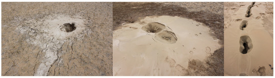
Figure 16.
The photos of liquefaction pits near the epicenter induced by the Maduo earthquake.
Third, the proposed methods had good performance regarding the Maduo earthquake. However, this area had natural landcovers or bare land; it is necessary to validate the performance of the proposed method in other places, such as the city.
5. Conclusions
Based on optical images from the GF-7 satellite, two machine learning methods (i.e., RF and GBDT) were proposed to detect the liquefaction that was induced by the 2021 Maduo Mw7.3 earthquake on the Tibetan Plateau. The final prediction accuracies of liquefaction were evaluated using the Kappa index, overall accuracy, recall score and precision score. Even with only forty-five training samples, the scores of the four evaluation indices reached about 0.9. By increasing the number of training samples, the performance was also improved. Furthermore, the spatial distribution predicted by RF and GBDT with 270 training samples was analyzed. Finally, the extracted liquefaction regions were overlapped on a pre-earthquake (GF-1D) and post-earthquake image (UAV) for comparison and validation. The spatial distribution of the extracted liquefaction pits was consistent with the information in previous studies. However, the number of liquefaction pits was larger than in the reported studies of other earthquakes. The high-resolution images, designed methods and geologic structures could be possible reasons. In summary, the proposed methods efficiently and quickly provided the spatial distribution of liquefaction based on post-earthquake satellite images, which could be helpful for earthquake intensity assessment and earthquake emergency response.
To the best of our knowledge, this study is the first to identify liquefaction based on random forest and gradient boosting decision tree methods with GF satellites. The proposed methods could be effective in taking advantage of optical satellite images and limited samples to identify liquefaction pits quickly after an earthquake. However, the weather could affect the timeliness of optical images, thus missing the optimal time to recognize the liquefaction pits. Furthermore, future studies will develop new extraction methods for liquefaction based on multi-source satellite data (e.g., different resolution optical satellite images, synthetic aperture radar images), optical satellite images with a time series long before the earthquake, and soil type information. Those further strategies could possibly overcome the shortcomings of the proposed methods for identifying liquefaction in this study. In addition, we will search for more data on other earthquakes to validate the replicability of the proposed methods.
Author Contributions
Conceptualization, Y.X. and P.L.; methodology, P.L.; software, P.L.; validation, Y.X.and P.L.; formal analysis, Q.T.; investigation, Y.X., W.L. and Y.Z.; resources, P.L.; data curation, Y.X.; writing—original draft preparation, P.L.; writing—review and editing, Y.X.; visualization, P.L.; supervision, Y.X.; project administration, P.L.; funding acquisition, Q.T. All authors have read and agreed to the published version of the manuscript.
Funding
This research was funded by National Key Research and Development Program of China (Grant No. 2021YFC3000601-3 and 2019YFE0108900), National Natural Science Foundation of China (Grant No. 42072248 and 42041006), Basic Research Program from the Institute of Earthquake Forecasting, China Earthquake Administration (Grant No. 2021IEF0505, CEAIEF20220102, and CEAIEF2022050502) and High-resolution Seismic Monitoring and Emergency Application Demonstration (Phase II) (Grant No. 31-Y30F09-9001-20/22), Research project of China Datang Corporation Ltd.—The active characteristics of the Naozhong fault in Tibet Yuqu River Zala Hydropower Station (DTXZ-02-2021).
Data Availability Statement
The data presented in this study are available from the corresponding author, Y.X. upon reasonable request.
Acknowledgments
The authors thank Tao Li from the Institute of Geology, China Earthquake Administration, Zhimin Li from the Qinghai Earthquake Agency, Zhaode Yuan from the Institute of Geology, China Earthquake Administration for their help during the fieldwork.
Conflicts of Interest
The authors declare no conflict of interest.
References
- Kramer, S.L. Geotechnical Earthquake Engineering; Prentice Hall: Hoboken, NJ, USA, 1996. [Google Scholar]
- Gihm, Y.S.; Kim, S.W.; Ko, K.; Choi, J.-H.; Bae, H.; Hong, P.S.; Lee, Y.; Lee, H.; Jin, K.; Choi, S.; et al. Paleoseismological Implications of Liquefaction-Induced Structures Caused by the 2017 Pohang Earthquake. Geosci. J. 2018, 22, 871–880. [Google Scholar] [CrossRef]
- Chini, M.; Albano, M.; Saroli, M.; Pulvirenti, L.; Moro, M.; Bignami, C.; Falcucci, E.; Gori, S.; Modoni, G.; Pierdicca, N.; et al. Coseismic Liquefaction Phenomenon Analysis by COSMO-SkyMed: 2012 Emilia (Italy) Earthquake. Int. J. Appl. Earth Obs. Geoinf. 2015, 39, 65–78. [Google Scholar] [CrossRef]
- Bhattacharya, S.; Hyodo, M.; Goda, K.; Tazoh, T.; Taylor, C.A. Liquefaction of Soil in the Tokyo Bay Area from the 2011 Tohoku (Japan) Earthquake. Soil Dyn. Earthq. Eng. 2011, 31, 1618–1628. [Google Scholar] [CrossRef]
- Huang, Y.; Yu, M. Review of Soil Liquefaction Characteristics during Major Earthquakes of the Twenty-First Century. Nat. Hazards 2013, 65, 2375–2384. [Google Scholar] [CrossRef]
- Liu-Zeng, J.; Wang, P.; Zhang, Z.H.; Li, Z.G.; Zhang, J.Y.; Yuan, X.M.; Wang, W.; Xing, X.C. Liquefaction in western Sichuan Basin during the 2008 Mw 7.9 Wenchuan earthquake, China. Tectonophysics 2017, 694, 214–238. [Google Scholar] [CrossRef]
- Cao, Z.Z.; Hou, L.Q.; Xu, H.M.; Yuan, X.M. Distribution and characteristics of gravelly soil liquefaction in the Wenchuan Ms 8.0 earthquake. Earthq. Eng. Eng. Vib. 2010, 9, 167–175. [Google Scholar] [CrossRef]
- Saraf, A.K.; Sinvhal, A.; Sinvhal, H.; Ghosh, P.; Sarma, B. Satellite Data Reveals 26 January 2001 Kutch Earthquake-Induced Ground Changes and Appearance of Water Bodies. Int. J. Remote Sens. 2002, 23, 1749–1756. [Google Scholar] [CrossRef]
- Ramakrishnan, D.; Mohanty, K.K.; Nayak, S.R.; Chandran, R.V. Mapping the Liquefaction Induced Soil Moisture Changes Using Remote Sensing Technique: An Attempt to Map the Earthquake Induced Liquefaction around Bhuj, Gujarat, India. Geotech. Geol. Eng. 2006, 24, 1581–1602. [Google Scholar] [CrossRef]
- Oommen, T.; Baise, L.G.; Gens, R.; Prakash, A.; Gupta, R.P. Documenting Earthquake-Induced Liquefaction Using Satellite Remote Sensing Image Transformations. Environ. Eng. Geosci. 2013, 19, 303–318. [Google Scholar] [CrossRef]
- Ishitsuka, K.; Tsuji, T.; Matsuoka, T. Detection and Mapping of Soil Liquefaction in the 2011 Tohoku Earthquake Using SAR Interferometry. Earth Planets Space 2012, 64, 1267–1276. [Google Scholar] [CrossRef]
- Baik, H.; Son, Y.-S.; Kim, K.-E. Detection of Liquefaction Phenomena from the 2017 Pohang (Korea) Earthquake Using Remote Sensing Data. Remote Sens. 2019, 11, 2184. [Google Scholar] [CrossRef]
- Belgiu, M.; Drăguţ, L. Random Forest in Remote Sensing: A Review of Applications and Future Directions. ISPRS J. Photogramm. Remote Sens. 2016, 114, 24–31. [Google Scholar] [CrossRef]
- Zhu, A.; Lu, G.; Liu, J.; Qin, C.; Zhou, C. Spatial Prediction Based on Third Law of Geography. Ann. GIS 2018, 24, 225–240. [Google Scholar] [CrossRef]
- Rashidian, V.; Baise, L.G.; Koch, M. Using High Resolution Optical Imagery to Detect Earthquake-Induced Liquefaction: The 2011 Christchurch Earthquake. Remote Sens. 2020, 12, 377. [Google Scholar] [CrossRef]
- Morgenroth, J.; Hughes, M.W.; Cubrinovski, M. Object-Based Image Analysis for Mapping Earthquake-Induced Liquefaction Ejecta in Christchurch, New Zealand. Nat. Hazards 2016, 82, 763–775. [Google Scholar] [CrossRef]
- Adriano, B.; Yokoya, N.; Miura, H.; Matsuoka, M.; Koshimura, S. A Semiautomatic Pixel-Object Method for Detecting Landslides Using Multitemporal ALOS-2 Intensity Images. Remote Sens. 2020, 12, 561. [Google Scholar] [CrossRef]
- Shafique, M. Spatial and Temporal Evolution of Co-Seismic Landslides after the 2005 Kashmir Earthquake. Geomorphology 2020, 362, 107228. [Google Scholar] [CrossRef]
- Zhu, A.X.; Liu, J.; Du, F.; Zhang, S.J.; Qin, C.Z.; Burt, J.; Behrens, T.; Scholten, T. Predictive Soil Mapping with Limited Sample Data. Eur. J. Soil Sci. 2015, 66, 535–547. [Google Scholar] [CrossRef]
- Yuan, Z.; Li, T.; Su, P.; Sun, H.; Ha, G.; Guo, P.; Chen, G.; Thompson Jobe, J. Large Surface-Rupture Gaps and Low Surface Fault Slip of the 2021 Mw 7.4 Maduo Earthquake Along a Low-Activity Strike-Slip Fault, Tibetan Plateau. Geophys. Res. Lett. 2022, 49, e2021GL096874. [Google Scholar] [CrossRef]
- McFEETERS, S.K. The Use of the Normalized Difference Water Index (NDWI) in the Delineation of Open Water Features. Int. J. Remote Sens. 1996, 17, 1425–1432. [Google Scholar] [CrossRef]
- Sengar, S.S.; Kumar, A.; Ghosh, S.K.; Wason, H.R.; Roy, P.S. Liquefaction Identification Using Class-Based Sensor Independent Approach Based on Single Pixel Classification after 2001 Bhuj, India Earthquake. J. Appl. Remote Sens. 2012, 6, 063531. [Google Scholar] [CrossRef]
- Acker, J.; Williams, R.; Chiu, L.; Ardanuy, P.; Miller, S.; Schueler, C.; Vachon, P.W.; Manore, M. Remote Sensing from Satellites☆. In Reference Module in Earth Systems and Environmental Sciences; Elsevier: Amsterdam, The Netherlands, 2014; ISBN 978-0-12-409548-9. [Google Scholar]
- Qi, J.; Chehbouni, A.; Huete, A.R.; Kerr, Y.H.; Sorooshian, S. A Modified Soil Adjusted Vegetation Index. Remote Sens. Environ. 1994, 48, 119–126. [Google Scholar] [CrossRef]
- Allbed, A.; Kumar, L.; Aldakheel, Y.Y. Assessing Soil Salinity Using Soil Salinity and Vegetation Indices Derived from IKONOS High-Spatial Resolution Imageries: Applications in a Date Palm Dominated Region. Geoderma 2014, 230–231, 1–8. [Google Scholar] [CrossRef]
- Xiao, J.; Shen, Y.; Tateishi, R.; Bayaer, W. Development of Topsoil Grain Size Index for Monitoring Desertification in Arid Land Using Remote Sensing. Int. J. Remote Sens. 2006, 27, 2411–2422. [Google Scholar] [CrossRef]
- Breiman, L. Random Forests. Mach. Learn. 2001, 45, 5–32. [Google Scholar] [CrossRef]
- Friedman, J.H. Greedy Function Approximation: A Gradient Boosting Machine. Ann. Stat. 2001, 29, 1189–1232. [Google Scholar] [CrossRef]
- Benediktsson, J.A.; Pesaresi, M.; Amason, K. Classification and Feature Extraction for Remote Sensing Images from Urban Areas Based on Morphological Transformations. IEEE Trans. Geosci. Remote Sens. 2003, 41, 1940–1949. [Google Scholar] [CrossRef]
- Zhao, C.; Qin, C.-Z. Identifying Large-Area Mangrove Distribution Based on Remote Sensing: A Binary Classification Approach Considering Subclasses of Non-Mangroves. Int. J. Appl. Earth Obs. Geoinf. 2022, 108, 102750. [Google Scholar] [CrossRef]
- Merghadi, A.; Yunus, A.P.; Dou, J.; Whiteley, J.; ThaiPham, B.; Bui, D.T.; Avtar, R.; Abderrahmane, B. Machine Learning Methods for Landslide Susceptibility Studies: A Comparative Overview of Algorithm Performance. Earth-Sci. Rev. 2020, 207, 103225. [Google Scholar] [CrossRef]
- Zhu, Z. Change Detection Using Landsat Time Series: A Review of Frequencies, Preprocessing, Algorithms, and Applications. ISPRS J. Photogramm. Remote Sens. 2017, 130, 370–384. [Google Scholar] [CrossRef]
- Seed, B. Landslides during earthquakes due to soil liquefaction. J. Soil Mech. Found. Div. 1968, 94, 1053–1122. [Google Scholar] [CrossRef]
- Wang, C.Y.; Dreger, D.S.; Wang, C.H.; Mayeri, D.; Berryman, J.G. Field relations among coseismic ground motion, water level change and liquefaction for the 1999 Chi-Chi (Mw = 7.5) earthquake, Taiwan. Geophys. Res. Lett. 2003, 30, 1–4. [Google Scholar] [CrossRef]


Publisher’s Note: MDPI stays neutral with regard to jurisdictional claims in published maps and institutional affiliations. |
© 2022 by the authors. Licensee MDPI, Basel, Switzerland. This article is an open access article distributed under the terms and conditions of the Creative Commons Attribution (CC BY) license (https://creativecommons.org/licenses/by/4.0/).