Abstract
Factory extraction from satellite images is a key step in urban factory planning, and plays a crucial role in ecological protection and land-use optimization. However, factory extraction is greatly underexplored in the existing literature due to the lack of large-scale benchmarks. In this paper, we contribute a challenging benchmark dataset named SFE4395, which consists of 4395 satellite images acquired from Google Earth. The features of SFE4395 include rich multiscale factory instances and a wide variety of factory types, with diverse challenges. To provide a strong baseline for this task, we propose a novel bidirectional feature aggregation and compensation network called BACNet. In particular, we design a bidirectional feature aggregation module to sufficiently integrate multiscale features in a bidirectional manner, which can improve the extraction ability for targets of different sizes. To recover the detailed information lost due to multiple instances of downsampling, we design a feature compensation module. The module adds the detailed information of low-level features to high-level features in a guidance of attention manner. In additional, a point-rendering module is introduced in BACNet to refine results. Experiments using SFE4395 and public datasets demonstrate the effectiveness of the proposed BACNet against state-of-the-art methods.
1. Introduction
Satellite building extraction is a spatially intensive task, which involves the process of inferring and distinguishing all background buildings in a given satellite image [1]. It plays a crucial role in urban planning, land-use change, environmental monitoring, and population estimation [2,3,4,5,6]. In recent years, with the development of satellite observation technology and the construction of smart cities the automatic extraction of buildings from satellite images has gradually become an important research topic and received the attention of many researchers. The extraction of some buildings, such as factories and dwellings plays a vital role in industrial planning and demographics but is neglected in existing works. In this paper, we focus on the problem of factory extraction based on satellite images, which is of great significance for protecting river and lake ecology and optimizing land space.
The research on extracting relevant buildings from satellite images started early, and traditional building-extraction methods [7,8,9] are usually based on manual design features. These methods mainly use design features such as the shape, spectrum, and contextual information of buildings in satellite images. Although these traditional building-extraction methods are credited with certain achievements, they also have shortcomings, such as low extraction accuracy and slow inference speed [10,11,12,13]. The main reason for these shortcomings is that handcrafted features are not robust for complex scenarios. In addition, the design of manual features requires multiple constraints on predefined features, which is time consuming and labor intensive. Therefore, traditional methods can no longer meet the speed and accuracy requirements of current technology for information acquisition. Fortunately, the emergence of deep learning methods [14,15] has greatly enhanced the bottlenecks faced by traditional methods, thus facilitating the development of the field of satellite building extraction. However, factory extraction is underexplored in the existing literature due to the lack of large-scale datasets.
To advance this research, we contribute a manually labeled dataset for factory extraction, called SFE4395. This dataset includes 4395 satellite images collected from Google Earth and covers various complex scenarios and factories. We present some typical examples from SFE4395 with different challenges in Figure 1. For instance, Figure 1a shows images and labels of factories located in dense building areas. Figure 1b presents a challenging scene in which the appearance of the different factories varies greatly. As shown in Figure 1c, haze above the factory remains an inevitable challenge that impairs the performance of factory extraction. Appearance contamination caused by long-term dust accumulation outside the factory or metal corrosion is also a serious challenge, as shown in Figure 1d. In addition, in order to accurately annotate the collected images, we use the road network map from Google Earth and Baidu Maps for mutual correction, and label buildings according to their names in the road network map. This approach greatly improves the accuracy of the labeling.
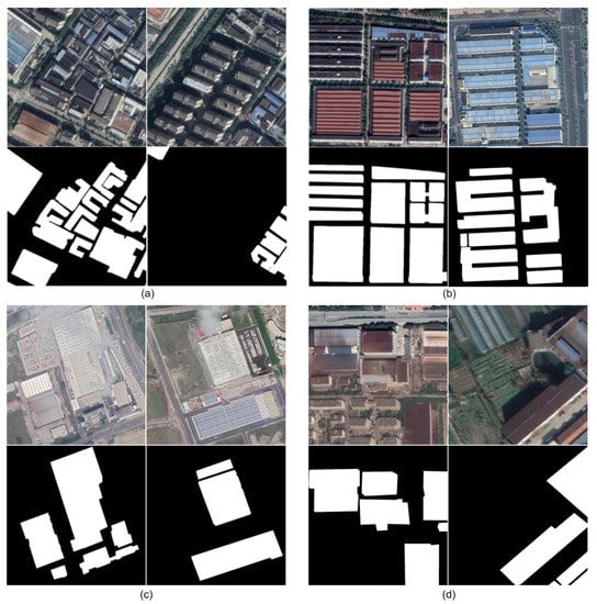
Figure 1.
Typical examples of images and labels from the SFE4395. (a) Two examples of dense buildings. (b) Factory with a considerable disparity in appearance. (c) Two haze occlusion images and a factory. (d) Typical representation of contaminated appearance.
The main characteristics of the SFE4395 dataset are as follows. (1) Rich, multi-scale factory instances. Different factory buildings produce large differences in size due to their different purposes, which involves richer, multiscale factory instances. (2) Wide variety of factory types. SFE4395 collects images from the industrial, suburban, and urban areas of 15 cities in China, with factories from different areas that have different characteristics in appearance and distribution, enriching the diversity of the factories. (3) Diverse challenges. We take into account the characteristics of satellite factory buildings and conclude that four challenging scenarios exist, which are dense building disturbance, complex background, haze occlusion, and appearance contamination. In addition, each image is annotated strictly according to the information provided by the road network map in Baidu Maps, and the annotated results are delivered to professionals for review before use.
We explore the accurate extraction of factory buildings from the collected satellite images. Initially, considering that factory extraction is a subtask of building extraction, we try to use general building-extraction methods to solve the task. After a comprehensive evaluation of various building-extraction methods with excellent performance, we select GMEDN [16] and DR-Net [17] for experimentation. However, their performance on the SFE4395 dataset is unsatisfactory, and Figure 2 shows some examples of incorrect and incomplete extraction. After an in-depth analysis, we believe that factory extraction faces many specific challenges, such as contaminated appearance and haze occlusion, but current building-extraction methods lack consideration of these challenging scenarios, thus resulting in degraded performance. To address these challenging scenarios, we propose a network for robust factory extraction, called BACNet, which is based on an encoder–decoder architecture. The network mainly consists of four stages: (1) the feature encoding stage, in which a novel bidirectional feature aggregation module is proposed, which is composed of a gated fusion module and a bidirectional concatenation operation. The gated fusion module performs selective information fusion on the multilayer features extracted from the network backbone, and then performs bidirectional concatenation operations with the output of ASPP to encode more global information. (2) To recover the detailed information loss caused by downsampling, we design a feature compensation module in the decoding stage, which combines the high-resolution features of the backbone and the output features of bidirectional feature aggregation module to generate preliminary prediction results. (3) Referring to the point-rendering [18] method, the generated preliminary segmentation results are iteratively upsampled, several segmentation difficulty points (e.g., boundary points) are selected among the results obtained from each upsampling, and point re-prediction is performed with the assistance of low-level, high-resolution features to optimize the inaccuracy of object edge segmentation. (4) There are often cluttered holes in the prediction results, which hurt the final performance. Considering the regular characteristics of factory buildings, we introduce a simple and effective post-processing method, hole filling [19], to improve this problem. In summary, the main contributions of this paper are as follows.

Figure 2.
Examples of prediction results of GMEDN and DR-Net in SFE439. In (a), from left to right are input image, prediction result of GMEDN, and label, respectively. In (b), input image, prediction result of DR-Net, and ground truth, respectively, are shown.
- A comprehensive satellite image dataset is presented for factory extraction, which includes 4395 satellite factory images collected from Google Earth with corresponding accurate annotations. In addition, we also classify all the images according to different challenging attributes, which will facilitate community research on specific building extractions.
- We propose a general segmentation network for factory extraction, in which a novel bidirectional feature aggregation module is designed to adaptively fuse multilayer features, and a simple and effective feature compensation module is proposed.
Extensive experiments and visualization results analysis on our SFE4395 dataset show the effectiveness of the proposed method, which is robust for complex scenarios and various types of factories. It achieves excellent performance in terms of F-measure and IoU metrics compared with existing segmentation methods. In addition, comparable performance is achieved on two publicly available building-extraction datasets—WHUBuilding and Inria—which demonstrates the effectiveness of our approach.
The rest of the article is as follows. The related work on semantic segmentation and building extraction is introduced in Section 2. In Section 3, we detail the contributed dataset and the details of the proposed network. Section 4 gives a series of experiments and analyses. Section 5 provides visualization of the results as well as analysis, and the last section concludes the whole paper.
2. Related Work
2.1. Semantic Segmentation Architecture
Semantic segmentation is a classical direction in the field of computer vision. With the development of deep learning [20,21,22,23,24] in recent years, this direction has rapidly progressed. Here, we classify the semantic segmentation methods based on deep learning into two categories: fully convolution based and candidate-region based.
The fully convolutional network (FCN) proposed by Long et al. [25] solves image segmentation at the semantic level for the first time by replacing the fully connected layers of the latter layers of the convolutional neural network used for classification with convolutional layers. To reduce the number of parameters and improve the efficiency of FCN, Badrinarayanan et al. [26] proposed SegNet, which innovatively uses the maximum pooling index to upsample the feature maps, resulting in a dramatic reduction in the number of parameters compared to FCN. In order to solve the problem of insufficient receptive fields in FCN, Chen et al. [27] proposed DeeplabV1, which used dilated convolution to increase the receptive field for the first time and also used a fully connected conditional random field at the end of FCN to improve accuracy. To improve the network’s ability to extract multiscale feature information, Chen et al. [28] proposed atrous spatial pyramid pooling (ASPP) in DeeplabV2 to sample the input feature maps at different atrous rates, which enhances the robustness of the network for multiscale object segmentation. DeeplabV3 [29] removes the dense conditional random field operation and improves the ASPP module to further enhance the segmentation performance. To optimize the problem of inaccurate boundary segmentation, Chen et al. [30] further proposed DeeplabV3+, based on DeeplabV3, by introducing a simple decoder operation, and the performance of the network for boundary segmentation improved.
The Mask R-CNN proposed by He et al. [31] is the first candidate-region-based segmentation model, which adds the prediction branch of Mask to Fast R-CNN [32] and proposes ROI alignment to solve the region misalignment problem caused by two quantizations in the ROI pooling operation. To solve the problem of scoring only the target-detection candidate region in Mask R-CNN, Huang et al. [33] proposed Mask Scoring RCNN, which added MaskIoU Head for scoring the segmentation mask and obtained better segmentation results.
2.2. Building Extraction
Because satellite images differ significantly from natural images, general semantic segmentation methods may not achieve satisfactory performance. Therefore, many semantic segmentation methods specifically for satellite image building extraction have been proposed in recent years.
Many researchers have started to apply this pixel-level prediction method to building extraction [34,35,36,37] from satellite images. For example, Guo et al. [38] designed an ensemble convolutional neural network based on the ensemble state-of-the-art CNN model to combine multiple feature extractors into a more powerful model. Because many proposed building-extraction methods are task-oriented and lack generality, Chen et al. [39] proposed a general deep deconvolutional neural network. This neural network consists of 27 convolutional and deconvolutional layers to implement pixel-level building extraction. Xu et al. [40] design a pixel-level segmentation network based on a deep residual network, which uses guided filtering to extract buildings from satellite images, and achieves outstanding performance in extracting buildings from different cities. In addition, the problem of partial missing and incomplete extraction of large buildings has been addressed. Shao et al. [41] proposed a residual refinement module to refine the prediction results, which significantly improves the accuracy of pixel-level prediction for large buildings.
In addition to these FCN-based variant methods, some methods focusing on multi-scale feature fusion have been proposed. For example, the global and multiscale encoder–decoder network proposed by Ma et al. [16] learns representative features of buildings by using global and local encoder. They also proposed a distilling decoder to explore information at different scales. In the same period, to solve the problem of detail information loss caused by pooling operations, Liu et al. [42] proposed the USPP network by integrating spatial pyramid pooling with an encoder–decoder architecture, and the model not only aggregates multiscale information, but also effectively recovers detailed information. However, these methods only perform the fusion of different features in the decoding stage, which is not conducive to feature extraction in the encoding stage. To solve this problem, Chen et al. [17] proposed DR-Net, which enables the fusion of different features in the encoding stage by introducing the dense Xception module in the encoder. Unfortunately, these approaches lack thought about feature fusion methods and ignore the semantic gap between different layers of features. Meanwhile, for the recovery of feature information, these methods are too simple and can cause the introduction of additional noise. However, our proposed BACNet solves these problems by introducing an efficient feature aggregation module and feature compensation module, which leads to better performance.
3. Materials and Methods
A new satellite dataset is introduced in this paper, which is the first to focus on factory extraction. In Section 3.1, we detail how the dataset is collected, the annotation method, and the statistics of distribution of this dataset. In Section 3.2, we propose a baseline method, called BACNet, which performs the best results so far on the task of factory extraction. In addition, we elaborate on the proposed network and describe the design of the loss function.
3.1. Dataset
3.1.1. Image Acquisition
The high clarity and real-time characteristics of WorldView-2 satellite images in Google Earth make it an attractive choice for us. Therefore, we chose the original images provided by the WorldView-2 satellite in Google Earth as the data source. Specifically, to ensure the diversity of factory types, we first collect a wealth of high-resolution satellite images from 15 cities in China. Note that in each city, we sample separately from three different types of regions—industrial, suburban, and urban—to further expand scene diversity. Moreover, as different types of factory buildings are used for different purposes, large differences in size are generated. Therefore, the images we acquire not only contain production factories of large building areas used for product processing and assembly, but also many other factories with small areas.
3.1.2. Image Annotation
Considering the efficiency of annotation, we directly annotate the collected high-resolution satellite images. In order to ensure that the targets in each image can be accurately labeled, we use the road network map in Google Earth and Baidu Maps of the same year as a guide and label the factory buildings in the image according to the building name in the road network map. Here we choose a professional Photoshop tool to achieve pixel-level annotation. After the manual annotation is completed, they are first checked by professionals to ensure the accuracy of the annotation results. Note that we use different colors to indicate different categories—white represents the factory and black denotes the background. After we crop the high-resolution images and corresponding label images in a sliding window manner, the above annotation is finished. Specifically, we set the window size to as the final image size, and set the sliding stride to 500 pixels, which can alleviate edge effects. Lastly, the semantic annotation information of each pixel is obtained through the corresponding transformation of by color and label.
3.1.3. Statistic and Analysis
After completing the above steps, we obtained 4395 images and labels. In order to sufficiently demonstrate the characteristics of the proposed dataset, we first analyze the challenges of factory extraction from two perspectives. First is the challenge of factory buildings themselves, i.e., the large difference in building styles between different cities and regions, and the multiscale problem caused by factory buildings for different purposes. The other is the influence of the surrounding environment on the factory buildings. After analyzing the collected satellite images, we summarize four main challenges, namely, dense building disturbance (DBD), haze occlusion (HO), appearance contamination (AC), and complex background (CB). DBD means that factory buildings are surrounded by a dense environment of other buildings, which makes it difficult for factory buildings to be accurately identified. HO refers to the fact that the factory buildings are obscured by high-altitude clouds and gases emitted by the factory, which destroys the integrity of the factory buildings. AC refers to the fact that the appearance of the factory buildings is contaminated by long-term dust accumulation and rusting, which causes different appearances for factories depending on the region in which they are located. CB is a natural challenge for satellite imagery, which can cause large intraclass differences in factory buildings. In Figure 3b, we show four examples of these challenges.
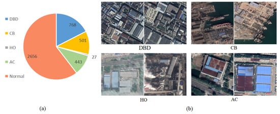
Figure 3.
SFE4395 dataset distribution statistics and examples. (a) Distribution of challenge attributes. (b) Typical examples of different challenge attributes. Herein, DBD, CB, HO and AC denote the dense building disturbance, complex background, haze occlusion, and appearance contamination, respectively.
Moreover, we denote the distribution of SFE4395 according to the challenges caused by the surrounding environment to the factory buildings. As shown in Figure 3a, approximately 60% of the data in SFE4395 belongs to less challenging factory satellite images, and approximately 40% of the data contains four specific challenges. In realistic scenarios, the challenges of the factory-extraction task are much more than that. Therefore, we manually divide the training and test sample of the SFE4395 dataset to be closer to the realistic scenarios. In particular, we take approximately 60% of the sample from each specific challenge as a testing sample, and the rest as a training sample. Then, we randomly select about 273 samples from the normal data to the testing set, and other samples are sent to the training set. Lastly, the number of samples in our training set and test set are 3077 and 1318, respectively, which satisfies the common split ratio of 7:3 for vision tasks.
3.2. Baseline Approaches
In this section, we will introduce the BACNet in detail, including the network architecture, bidirectional feature aggregation module, feature compensation module, point-rendering module, hole-filing method, and loss function details.
3.3. Overview of Architecture
Figure 4 presents the overall proposed network structure, which is based on an encoder–decoder segmentation network. The encoder consists of a backbone, ASPP, and a bidirectional feature aggregation module. The decoder includes two parts: feature compensation module and point-rendering module. For the task of factory extraction, factories with different sizes are difficult to accurately classify in terms of the features of a single receptive field. Therefore, an ASPP module is adopted in the feature encoding stage to obtain multireceptive field features. This module samples the given input in parallel with the dilated convolution at different sampling rates, which are 1, 6, 12, and 18 respectively. However, the detailed information of low-level features is also critical for the dense prediction task, such as factory extraction, which is ignored in the ASPP module. To this end, we design a bidirectional feature aggregation module in the encoder to perform bidirectional information aggregation on the output of the ASPP module and the multi-level features extracted from the backbone (i.e., ResNet-101 [43]). Due to difference of feature scales, the information loss inevitable occurs in the downsampling operation of feature aggregation. Therefore, the feature compensation module is proposed to compensate for the lost information by incorporating high-resolution original features (i.e., , ). Moreover, the refinement of prediction results is a key step in the segmentation task; thus, we design a hole-filling technique to handle irregular small holes appearing in the interior of an object, and introduce a point-rendering module to optimize the inaccurate edge segmentation. In the following sections, we will introduce these modules in detail.
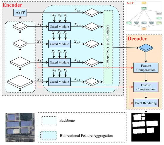
Figure 4.
Overall framework of BACNet.
3.3.1. Bidirectional Feature Aggregation Module
Rich, multiscale information is quite important in the task of factory extraction. Although the ASPP module can provide high-level features with multiple receptive fields, it usually has a lower resolution, which is not conducive to the segmentation of small objects. To this end, an intuitive idea is to use high-resolution, low-level features to compensate for the detailed information in the high-level features. Unfortunately, simple combination strategies (e.g., addition and concatenation) cannot deal with the large amount of redundant and noise information in multilayer features, which severely threatens the segmentation performance.
Therefore, inspired by GFF [44], we propose a bidirectional feature aggregation module to mitigate this issue in the encoding phase, which consists of two parts: a gated fusion module and a bidirectional concatenation operation. The gated fusion module is used for selective information fusion of multilayer features, such that each layer is enhanced by the other layers’ effective information. Meanwhile, the noise in the fusion process is significantly reduced due to the use of the mature gate technique. Carefully, given L feature maps extracted from the backbone network, each level i is associated with a gate map . With these gate maps, the fusion process can be defined as
where is the fused feature map for the ith level, × denotes the element-wise multiplication in the channel dimension, and each gate map is computed from the convolution layer with parameters of . The detailed operation is shown in Figure 5.
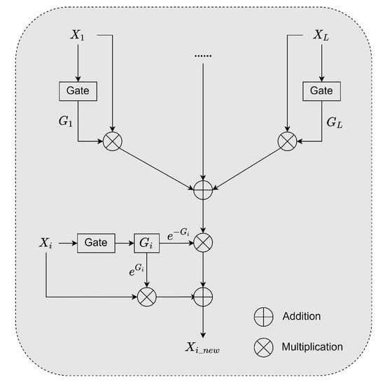
Figure 5.
The structure of the gated fusion module.
It is worth noting that the propagation of the feature at location in the j layer to the location in the i layer is jointly determined by the two gate maps . The represents that the feature at location in the j layer is effective information, but this information will be propagated to the same location at layer i only when the . This design ensures that the advantage features the location of the current layer and is not covered by the other layer features, whereas the location of the disadvantage features will be improved by the advantages of the information of the other layers.
In addition, to encode more global information, and inspired by the fact that dense concatenation operation can enhance feature propagation, we use a bidirectional dense concatenation operation for multilevel feature output from the gated fusion and ASPP modules, as shown in Figure 6. Specifically, we use dense bottom-up and top-down concatenation for multilayer features, respectively, which allows the model to encode rich, multiscale information and better handle factories of different sizes.
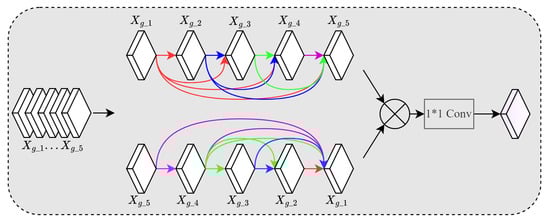
Figure 6.
Bidirectional concatenation module.
3.3.2. Feature Compensation Module
The bilinear interpolation technique in Deeplabv3+ is used to directly recover from the output features of the decoder to the final prediction results, which ignores that the low-resolution semantic features lose a great deal of detailed information. Therefore, it is necessary to recover lost information in the decoding stage, which will improve the final prediction performance.
To this end, we introduce an feature compensation module to recover detailed information lost in the output features of the bidirectional feature aggregation module. This method only increases a small amount of computation compared with the direct bilinear interpolation approach but achieves better results. As shown in Figure 7, the feature compensation module receives both low-resolution and high-resolution feature maps as input. We first perform twofold upsampling on the , and then we use with rich detailed information as compensate features, and finally adopt the concatenation operation in the channel dimension to fuse the two features. Although the feature detailed information, it also introduces noisy features due to the weak semantic discrimination of low-level features. Therefore, we attempt to highlight effective information and suppress noise through the mature attention technique CBAM [45] in the feature-compensation module. The fused features sequentially perform channel attention and spatial attention to obtain refined features, which are then added to the original features as residuals. Therefore, the feature compensation module can be formulated as follows:
where U and denote twofold upsampling and concatenation operations, respectively. H denotes a convolution layer, and represent channel attention and spatial attention, respectively, and y represents the output of feature-compensation module.
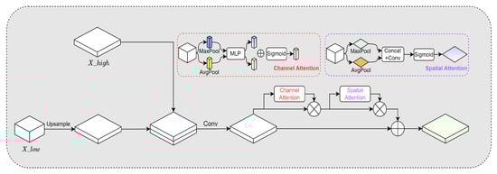
Figure 7.
Feature-compensation module.
It must be noted that in BACNet, we use the feature-compensation module twice. In the first instance, represents the low-resolution feature map output from the bidirectional feature aggregation module of the encoder, represents the second-layer high-resolution feature extracted from the backbone. In the second instance, represents the output result of the first feature-compensation module, and denotes the first layer of high-resolution feature extracted by the backbone.
3.3.3. Point Rendering Module
In the decoder, due to the limitation of resolution, we only restore the output features of the encoder to 1/4 the size of the input image by using the feature compensation module. Therefore, in order to obtain the prediction result size consistent with the input image size, we introduce the point-rendering method for the last step of recovery. This method mitigates the undersampling problem by analogy with the rendering problem in computer graphics, which is widely used for instance and semantic segmentation tasks [46,47,48,49].
We take the output features of the feature compensation module and the low-level features as coarse prediction results and the fine-grained features, respectively. Then, the N points are selected from the coarse prediction results by using the subdivision strategy [50], which provides the location information of value that is significantly different from its neighbors. Therefore, these points usually move toward the uncertain regions, such as object edges. To refine the coarse predictions, we simultaneously extract features corresponding to these points from fine-grained feature and coarse prediction, which are concatenated and sent to a multilayer perception to improve prediction results of these points. Finally, the coarse prediction result is updated by these improved point features. Note that we set N to 1024 and 8096 for the training and testing phase respectively, which achieves a balance between performance and efficiency.
3.3.4. Hole Filing
The prediction results usually contain some irregular small holes, which hinders the performance of factory extraction. Considering that the shape of factory buildings is generally regular, these holes cannot be factory regions according to prior knowledge. Therefore, we use the hole-filling post-processing technique to solve this issue. Specifically, for each predicted segmentation result, the hole filling first reads the image as a grayscale image and counts the number of pixels in all connected regions. Then, connected regions with a pixel count less than a certain threshold of 1000 are considered as background. This is a simple and effective refinement method and is validated in the experimental section.
3.4. Loss Function
The loss function is important in model optimization, and it determines the final segmentation effect in the factory-extraction task.
In BACNet, the loss function includes two items:
- Loss_image: The cross-entropy between the semantic segmentation result and ground truth.
- : The cross-entropy between the result of point prediction in the point-rendering module and ground truth.
For the , the goal is to learn intuitively for BACNet, so that the factory-extracted result is closer to the ground truth. For a sample, assuming the width and height are W and H, respectively, the total number of pixels is , for pixel i, the probability of its classification as factory is . If the pixel is labeled as a factory in the ground truth, the pixel is labeled ; otherwise, the pixel is labeled as . is defined as follows:
The purpose of is to make point rendering more accurate in predicting difficult points. Suppose the number of selected points is N. For a single point i, the probability that it is predicted to be a factory is . If the point is classified as a factory in the ground truth, then , otherwise . is defined as follows:
The total loss function of the whole model, , is represented by equation 6,
4. Experimental Results and Analysis
In order to evaluate the performance of the proposed model, we conduct a large number of experiments to validate it. In this section, we describe in detail the evaluation metrics, the implementation details, comparisons between different models, evaluation of the effectiveness of other datasets, and ablation experiments for different modules.
4.1. Evaluation Metrics
There are four widely used metrics for segmentation performance evaluation in semantic segmentation tasks, namely, precision, recall, intersection over union (IoU), and F-measure. Therefore, in this paper we use these metrics to perform a comprehensive performance evaluation.
In our task, true positive (TP) represents the number of factory pixels predicted successfully as the positive class, true negative (TN) represents the number of background pixels predicted successfully as the negative class, false positive (FP) represents the number of negative class pixels predicted as positive, which means background pixels are classified as factory, and false negative (FN) represents the number of factory pixels classified as background, and is a predefined parameter that is set to 1 in this paper.
- Precision. The ratio of the number of samples accurately classified as a positive class to the number of all samples classified as positive class. This means that the prediction results in a number of samples of the positive class are really positive; it is calculated as follows:
- Recall. Recall is a measure of the probability of a class of pixels being correctly predicted, i.e., the ratio of the number of pixels correctly predicted by using that class to the total number of pixels belonging to that class in the ground truth, which is calculated as follows:
- Intersection over union (IoU). IoU is a standard metric for semantic segmentation tasks. It compares the similarity between predicted result and ground truth by the intersection and merge ratios. The larger the IoU value, the higher the similarity:
- F-measure. Precision and recall sometimes appear to contradict each other. In order to consider them together, the two indicators are weighted and averaged to obtain the F-measure, and a larger value of F indicates a more effective model, calculated as follows:
4.2. Implementation Details
Our network is based on DeeplabV3+ improvement, replacing the original backbone network Xception [51] with ResNet101 to extract more powerful feature representations from input images. The model is initialized by the parameters of the pre-trained model of ResNet101, which speeds up the convergence of the model. We use PyTorch to build this model, and choose the standard stochastic gradient descent (SGD) [52] as an optimizer. Specifically, we set the initial learning rate to , and epoch number to 60. To alleviate the overfitting problem, the hyper-parameter is used to update the learning rate every three epochs to achieve learning rate decay. In addition, all experiments are performed under Linux OS and accelerated with GeForce RTX 3090 for training and validation, where the GPU acceleration libraries are CUDA11.1 and cuDNN8.2. To better utilize the label images, we employ 1 and 0 to represent all pixels with pixel values [255,255,255] and [0,0,0] respectively.
4.3. Evaluation on Different Datasets
In this section, we validate the performance of BACNet on SEF4395 and the publicly available building-extraction dataset WHUBuilding and Inria, respectively.
4.3.1. Evalution on SFE4395
We compare five general semantic segmentation methods, including U-Net [53], PSPNet [54], DeeplabV3+, HRNet-FCN [55], and EMANet [56]. Moreover, two latest building-extraction methods, GMEDN and DR-Net, are also compared. For the sake of fairness, these models are trained and tested with consistent parameters under the experimental environment of Section 4.2.
Comparison with Baseline Method. Here, the DeeplabV3+ based on the ResNet101 network is used as the baseline, and its performance is shown in the third row of Table 1. It can be seen that BACNet achieves 6.57% and 3.82% improvement on IoU and F-measure, respectively, which proves that our proposed method is more effective compared to the baseline.

Table 1.
Precision, recall, IoU, and F-measure of different methods counted by the SFE4395 dataset.
Comparison with other methods. From the observation of Table 1, it is obvious that the proposed BACNet performs best in both IoU and F-measure. Among all of the comparisons, the performance of PSPNet and GMEDN perform poorly. As a whole, the proposed BACNet achieves 89.37% in IoU and 94.37% in F-measure. Compared to other methods, the improvement of IoU by BACNet is, respectively, 6.55% (U-Net), 9.14% (PSPNet), 5.42% (HRNet-FCN), 2.03% (EMANet), 9.51% (GMEDN), and 3.88% (DR-Net). Enhancements of BACNet on F-measure are 3.85% (U-Net), 5.37% (PSPNet), 3.13% (HRNet-FCN), 2.31% (EMANet), 5.7% (GMEDN), and 1.95% (DR-Net). These surprising results demonstrate the effectiveness of BACNet for factory-extraction task.
Comparison of visual results. Apart from the numerical results, as shown in Figure 8, the visual difference between the different methods is also more obvious. For example, a variety of factory buildings of different scales exist in the second row of Figure 8, including some small factories. The other four methods generally suffer from inaccurate extraction of small factories. However, our method obtains more accurate results in extracting such factories. Moreover, the factory distribution in the third row in Figure 8 is more dense. Compared with the prediction results of the other methods, the advantage of BACNet in predicting target contours and edges is more prominent in such scenarios. In addition, for the haze occlusion problem in the fifth row of Figure 8, the prediction results of other methods are heavily influenced by haze; only our method achieves the most satisfying visual effects.
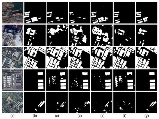
Figure 8.
Example comparison of prediction results with other methods on the SFE4395 dataset. (a) Input image. (b) Ground truth. (c) HRNet-FCN. (d) EMANet. (e) GMEDN. (f) DR-Net. (g) BACNet.
We analyze the above phenomenon and make the following explanations. As we all know, multi-scale information is crucial for the task of satellite image factory extraction. These several popular methods, while using more or less multiscale information, usually have two drawbacks. One is that the multiscale information is not fully utilized; for example, PSPNet only uses spatial pyramid pooling for the deepest features, ignoring useful information in other layers. EMANet applies the expectation-maximizing attention module only to single-layer features, without taking advantage of the scale of information brought by other layers. Secondly, the fusion of multiscale information is too simple; for example, HRNet-FCN uses simple addition for feature fusion at different scales, and GMEDN uses a concatenation operation to fuse. They both ignore the semantic gap generated by direct fusion between different feature maps. BACNet not only makes full use of multiscale information, but also designs an effective fusion method.
In addition, in order to obtain richer global information, these methods use a large number of downsampling operations to increase the receptive field during feature extraction. However, the use of the downsampling operation inevitably reduces the size of the feature map, resulting in the loss of the original image detail information. These methods do not focus on the effective recovery of detailed information. For example, DR-Net and EMANet quadruple upsampling of low-resolution predictions directly, and GMEDN uses de-convolution operations on the decoded result to achieve feature recovery. They all ignore the recovery of detailed information; thus, it is difficult to obtain satisfactory results on edges, contours, etc. In contrast to them, BACNet carefully designs a feature compensation module for feature information recovery, and combines point rendering to further optimize detailed information. As a result, the most satisfying results are produced.
4.3.2. Evaluation on Other Datasets
The effectiveness of BACNet has been proven for factory-extraction tasks, but the ability to extract other building types is still unknown. To measure the effectiveness of BACNet on other datasets, we conduct experiments on two publicly available building-extraction datasets, WHUBuilding and Inria, and compare the performance with other methods. As seen in Table 2, BACNet achieves 87.79% of IoU and 92.55% of F-measure in the WHUBuilding dataset, achieving a performance comparable to other advanced methods. Table 3 shows the performance of different methods for building extraction in different regions of the Inria dataset, with BACNet achieving excellent performance. This proves that our method can not only solve the extraction of factory buildings, but also has strong effectiveness to solve the general building extraction.
Table 2.
IoU and F-measure of different methods in WHUBuilding dataset.
Table 3.
IoU of different methods in Inria dataset.
We carefully analyze the reasons for the effectiveness of BACNet on these datasets. Two challenges are always faced for general building extraction; one is that nonbuilding objects are similar to buildings, and the other is that buildings vary greatly in size and shape. However, these challenges can be solved by our approach. Because the gated fusion module in bidirectional feature aggregation, the module adaptively fuses the features of different layers, so that the high-level semantic information and the low-level detail information are effectively fused; thus, the similarity problem between non-building and buildings is solved. Meanwhile, the bidirectional concatenation operation enables the model to focus on buildings of different scales, solving the challenge of large size differences.
4.4. Ablation Experiments
As mentioned in Section 3.2, BACNet is mainly composed of four modules, bidirectional feature aggregation module, feature compensation module, point rendering, and HF. In order to study their contribution to the factory building-extraction task, we design several sets of experiments to complete the factory extraction respectively. They are
- Net1: Baseline. The DeeplabV3+ network with ResNet101 as the backbone is used for training and testing in this experiment;
- Net2: Baseline + Point Rendering. Replacing the final up-sampling operation in DeeplabV3+ decoder with Point Rendering module;
- Net3: Baseline + Point Rendering + HF. Adding HF module to the prediction results of Net2 for experiment;
- Net4: Baseline + Point Rendering + HF + BFAM. Adding bidirectional feature aggregation module to the encoder based on Net3;
- Net5: Baseline + Point Rendering + HF + BFAM + FCM. Feature compensation module is introduced in the decoder, the rest is the same as the Net4 setting.
In the experimental setup, BFAM represents the bidirectional feature aggregation module, FCM stands for feature compensation module, and HF represents hole filling. As shown in Table 4, “√” indicates the module used in the experiment.
Table 4.
Performance of different modules on the test set. “√” means the module is used in this experiment.
Note that the experimental settings of the networks in this section are the same as those mentioned in Section 4.2. Moreover, because the SFE4395 dataset is divided into five categories according to different challenge attributes, we use the average of the prediction scores of these categories for comparison.
It can be seen from Table 4 that with the addition of different modules, the model performs better in both IoU and F-measure metrics that we focus on. Specifically, Net1 has the worst performance of all the networks compared, because it is only the most basic DeeplabV3+ network. For the point-rendering and HF modules, their effectiveness has been demonstrated in previous work, which also coincides with the experimental results of Net2 and Net3. Thanks to the use of bidirectional feature aggregation module, Net4 obtains a more superior performance, which proves the effectiveness of bidirectional feature aggregation module in encoder. After integrating all the submodules, Net5 achieves the best performance, with IoU reaching 88.97% and F-measure reaching 94.15%. These results show that each module can contribute positively to our proposed BACNet model.
To more clearly reflect the advantages of BACNet, we also show the differences between baseline and our method in IoU and F-measure on different challenge subsets, as shown in Figure 9. Specifically, BACNet outperforms the baseline approach in all challenge subsets, which brings a significant improvement over baseline methods when faced with the challenges of dense building occlusion and complex backgrounds, which proves the advantage of BACNet.
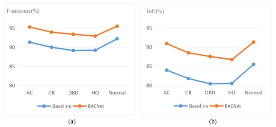
Figure 9.
Performance comparison of BACNet and baseline. (a) Results of F-measure. (b) Results of IoU.
Moreover, we do an in-depth discussion and analysis of how BACNet achieves excellent performance under different challenges. The problem of indistinguishable factory boundaries caused by the dense distribution of buildings, the model needs more detailed boundary information, and the compensation of rich, detailed information in the feature compensation module solves this difficulty. For factory-building truncation caused by haze occlusion, the model must rely on the semantic information of the high layers, which alleviates this problem by highlighting the bottom-up concatenation in the bidirectional concatenation operation. Factory buildings suffer from a lot of dust or rust due to long-term exposure, which in turn causes a large difference in the appearance of different areas of the factory. To solve this problem, the model must focus not only on high-level features but also a large receptive field. BACNet uses ASPP to capture features with different receptive fields and uses bottom-up concatenation to highlight high-level features, thus improving the performance of the network with regard to this challenge. For the challenge of a complex background, it is not enough for the model to have the ability to extract high-level features. It must also have the ability to recover detailed information. The feature compensation module makes the model have powerful detail recovery ability by using low-level feature information to compensate high-level features.
At the same time, as shown in Figure 10, each module produces a large visual improvement, with the red rectangular area being the most obvious. For example, the baseline approach is more disturbed by buildings similar to the factory (see the red rectangular box in the third column in Figure 10c), whereas the introduction of point rendering, the bidirectional feature aggregation module, and the feature compensation module largely optimizes this problem (red rectangle in the third column of Figure 10d–f). In addition, for the presence of irregular small holes in the prediction results, the use of hole filling solves this difficulty (see the third column in Figure 10e).
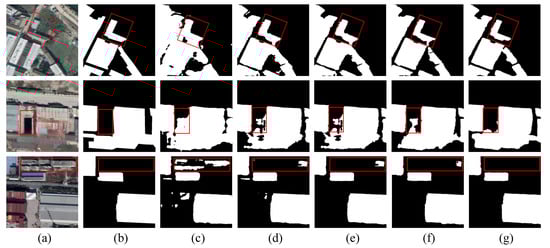
Figure 10.
Visualization of segmentation results of three images using different modules. Column (a) shows the three input images. Column (b) lists the ground truth. Columns (c–g) show the prediction results of Net1-5.
In addition, we also validate the effectiveness of bidirectional feature aggregation module over GFF on our test dataset with different challenges, Figure 11a shows the F-measure and Figure 11b shows the IoU. The results show that bidirectional feature aggregation module leads GFF across the board in the factory-extraction task. Specifically, bidirectional feature aggregation module delivers different enhancements on different subsets of challenges. Compared to the weak improvement in normal and complex background challenges, the improvement brought by the bidirectional feature aggregation module for the haze occlusion, appearance contamination and dense building disturbance challenge is quite substantial.
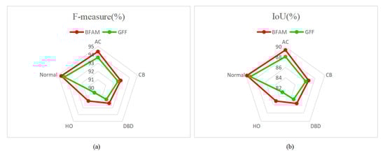
Figure 11.
Performance comparison of BFAM and GFF. (a) Results in F-measure, (b) Results in IoU.
Moreover, we also perform detailed comparative experiments on which features are used in the feature compensation module. From Table 5, it can be seen that the best performance is achieved by using and as feature compensation. Because the purpose of feature compensation is to recover the detailed information of high-level features lost in multiple downsampling, it is natural to use high-resolution features rich in detail information as compensation. , , as the first two features extracted from the backbone, have the richest detailed information compared to other high-level features, and thus achieve the best performance.
Table 5.
Performance of using different features as compensation on the test set. “√” means the feature is used in this experiment.
5. Visualization Results
To more intuitively reflect the promoting effect of the bidirectional feature aggregation module and feature compensation module for the factory-extraction task, we visualize the feature responses of BACNet with different modules through the use of the gradient-weighted class activation mapping (GradCAM) [57] technique. In Figure 12, we present some typical examples for comparison the influence of different modules, where the different colors represent the different degrees of attention. Deeper colors indicate higher confidence in the region. Specifically, we show the feature response of the baseline, the baseline with bidirectional feature aggregation module, the baseline with bidirectional feature aggregation module, and the feature compensation module in the (b), (c), and (d) of Figure 12, respectively. As shown in Figure 12b, the responses of factory buildings are usually sparse and incomplete, which will lead to worse segmentation results. When the bidirectional feature aggregation module is introduced into the baseline, it can be seen that the more dense response of all factory buildings in satellite images, as shown in Figure 12c, will improve the prediction results. Therefore, this phenomenon can better prove the effectiveness of the bidirectional feature aggregation module.
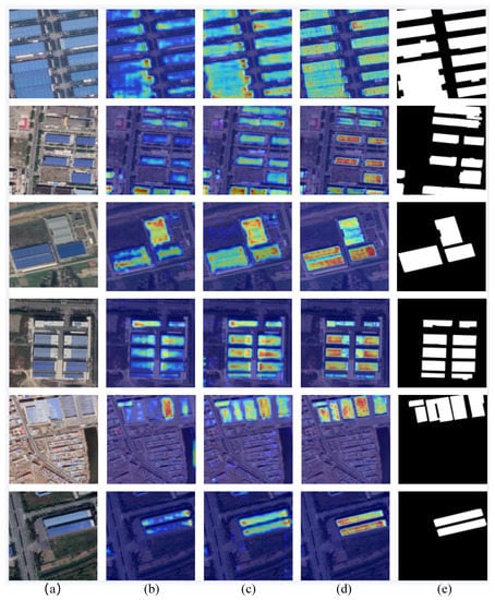
Figure 12.
Visualization results of different modules. (a) Original images. (b) Before bidirectional feature aggregation module. (c) After bidirectional feature aggregation module. (d) After bidirectional feature aggregation module and feature compensation module. (e) Ground truth.
Although the bidirectional feature aggregation module brings some improvement over the baseline method, it is hard to handle the edge and the interior segmentation issue of factory buildings. For example, the second row of Figure 12c is not strong enough for the extremely obvious factories in the internal responses, and the corresponding feature responses in the sixth row suffers from the same problem. In addition, the feature responses for the factory edges in the fourth and sixth rows of Figure 12c are poor. To this end, the feature compensation module is used in the baseline method. Figure 12e shows that it can significantly improve both responses in the edge and interior of factory buildings. For instance, the second and sixth rows of Figure 12d not only achieve a strong response to the interior of the factory, but also the edge details are better highlighted, which bring surprising visual improvement.
6. Conclusions
This paper introduces a satellite image factory-extraction task, which is of great significance for improving ecological protection and land-use optimization. To the best of our knowledge, we contribute the first dataset for factory extraction, and provide five challenging, labeled attribute subsets with pixel-level annotation for each image. In addition, we propose a baseline method BACNet for satellite image factory building extraction. In particular, we design two simple and effective modules, including a bidirectional aggregation module for adaptively aggregating effective contextual information from different layers, and a feature compensation module for recovering information lost in the downsampling operation. Experimental results demonstrate that the proposed method is superior to existing methods on the proposed factory-extraction dataset.
However, there are two limitations to our approach. First, the bidirectional dense concatenation operation in bidirectional feature aggregation module is more focused on high-level features, which causes the network to perform poorly for small-scale targets. To solve this problem, we will explore how to better balance high-level and low-level features, thereby improving the model to handle the problem of building extraction at arbitrary scales. Another limitation is that BACNet inevitably increases the time overhead in multilayer feature fusion, which affects the prediction speed of the network. To solve this problem, we will think about further simplifying the fusion of multilayer features.
Author Contributions
Conceptualization, Y.D. and A.L.; methodology, Y.D.; validation, A.L., C.L. and B.L.; formal analysis, Y.D. and A.L.; investigation, Y.D., W.L. and A.L; resources, Y.D., C.L. and B.L.; data curation, Y.D., W.L. and A.L.; writing—original draft preparation, Y.D. and A.L.; writing—review and editing, A.L., C.L. and B.L.; visualization, Y.D. and A.L.; supervision, A.L., C.L. and B.L.; funding acquisition, C.L. and B.L. All authors have read and agreed to the published version of the manuscript.
Funding
This research is funded by Joint Funds of the National Natural Science Foundation of China (No. U20B2068), The University Synergy Innovation Program of Anhui Province (No.GXXT-2020-015, No.GXXT-2021-065) and Natural Science Foundation of Anhui Higher Education Institution (KJ2020A0040).
Data Availability Statement
Our code and FE4395 daaset can be found here: https://github.com/mmic-lcl/Datasets-and-benchmark-codes.
Acknowledgments
The authors would like to show their gratitude to the editors and the anonymous reviewers for their comments and suggestions.
Conflicts of Interest
The authors declare no conflict of interest.
References
- Yang, H.; Wu, P.; Yao, X.; Wu, Y.; Wang, B.; Xu, Y. Building Extraction in Very High Resolution Imagery by Dense-Attention Networks. Remote Sens. 2018, 10, 1768. [Google Scholar] [CrossRef]
- Zhang, L.; Dong, R.; Yuan, S.; Li, W.; Zheng, J.; Fu, H. Making low-resolution satellite images reborn: A deep learning approach for super-resolution building extraction. Remote Sens. 2021, 13, 2872. [Google Scholar] [CrossRef]
- Chen, X.; Qiu, C.; Guo, W.; Yu, A.; Tong, X.; Schmitt, M. Multiscale feature learning by transformer for building extraction from satellite images. IEEE Geosci. Remote. Sens. Lett. 2022, 19, 1–5. [Google Scholar] [CrossRef]
- Wang, H.; Miao, F. Building extraction from remote sensing images using deep residual U-Net. Eur. J. Remote. Sens. 2022, 55, 71–85. [Google Scholar] [CrossRef]
- Wang, Y.; Zeng, X.; Liao, X.; Zhuang, D. B-FGC-Net: A Building Extraction Network from High Resolution Remote Sensing Imagery. Remote Sens. 2022, 14, 269. [Google Scholar] [CrossRef]
- Zorzi, S.; Bazrafkan, S.; Habenschuss, S.; Fraundorfer, F. PolyWorld: Polygonal Building Extraction with Graph Neural Networks in Satellite Images. In Proceedings of the IEEE/CVF Conference on Computer Vision and Pattern Recognition, New Orleans, LA, USA, 18–24 June 2022; pp. 1848–1857. [Google Scholar]
- Katartzis, A.; Sahli, H.; Nyssen, E.; Cornelis, J. Detection of buildings from a single airborne image using a Markov random field model. In Proceedings of the IGARSS 2001. Scanning the Present and Resolving the Future. Proceedings. IEEE 2001 International Geoscience and Remote Sensing Symposium (Cat. No. 01CH37217), Sydney, Australia, 9–13 July 2001; IEEE: New York, NY, USA, 2001; Volume 6, pp. 2832–2834. [Google Scholar]
- Zhang, L.; Huang, X.; Huang, B.; Li, P. A pixel shape index coupled with spectral information for classification of high spatial resolution remotely sensed imagery. IEEE Trans. Geosci. Electron. 2006, 44, 2950–2961. [Google Scholar] [CrossRef]
- Jin, X.; Davis, C.H. Automated building extraction from high-resolution satellite imagery in urban areas using structural, contextual, and spectral information. EURASIP J. Adv. Signal Process. 2005, 2005, 1–11. [Google Scholar] [CrossRef]
- Xie, Y.; Zhu, J.; Cao, Y.; Feng, D.; Hu, M.; Li, W.; Zhang, Y.; Fu, L. Refined extraction of building outlines from high-resolution remote sensing imagery based on a multifeature convolutional neural network and morphological filtering. IEEE J. Sel. Top. Appl. Earth Obs. Remote. Sens. 2020, 13, 1842–1855. [Google Scholar] [CrossRef]
- Liao, C.; Hu, H.; Li, H.; Ge, X.; Chen, M.; Li, C.; Zhu, Q. Joint learning of contour and structure for boundary-preserved building extraction. Remote Sens. 2021, 13, 1049. [Google Scholar] [CrossRef]
- Tomljenovic, I.; Höfle, B.; Tiede, D.; Blaschke, T. Building extraction from airborne laser scanning data: An analysis of the state of the art. Remote Sens. 2015, 7, 3826–3862. [Google Scholar] [CrossRef]
- Zhou, D.; Wang, G.; He, G.; Long, T.; Yin, R.; Zhang, Z.; Chen, S.; Luo, B. Robust building extraction for high spatial resolution remote sensing images with self-attention network. Sensors 2020, 20, 7241. [Google Scholar] [CrossRef] [PubMed]
- Hossain, M.D.; Chen, D. A hybrid image segmentation method for building extraction from high-resolution RGB images. ISPRS J. Photogramm. Remote. Sens. 2022, 192, 299–314. [Google Scholar] [CrossRef]
- Yin, J.; Wu, F.; Qiu, Y.; Li, A.; Liu, C.; Gong, X. A Multiscale and Multitask Deep Learning Framework for Automatic Building Extraction. Remote Sens. 2022, 14, 4744. [Google Scholar] [CrossRef]
- Ma, J.; Wu, L.; Tang, X.; Liu, F.; Zhang, X.; Jiao, L. Building extraction of aerial images by a global and multi-scale encoder-decoder network. Remote Sens. 2020, 12, 2350. [Google Scholar] [CrossRef]
- Chen, M.; Wu, J.; Liu, L.; Zhao, W.; Tian, F.; Shen, Q.; Zhao, B.; Du, R. DR-Net: An improved network for building extraction from high resolution remote sensing image. Remote Sens. 2021, 13, 294. [Google Scholar] [CrossRef]
- Kirillov, A.; Wu, Y.; He, K.; Girshick, R. Pointrend: Image segmentation as rendering. In Proceedings of the IEEE Conference on Computer Vision and Pattern Recognition, Seattle, WA, USA, 16–20 June 2020; pp. 9799–9808. [Google Scholar]
- Zhao, W.; Gao, S.; Lin, H. A robust hole-filling algorithm for triangular mesh. Vis. Comput. 2007, 23, 987–997. [Google Scholar] [CrossRef]
- Li, C.L.; Lu, A.; Zheng, A.H.; Tu, Z.; Tang, J. Multi-adapter RGBT tracking. In Proceedings of the 2019 IEEE International Conference on Computer Vision Workshop (ICCVW), Seoul, Korea, 27–28 October 2019; pp. 2262–2270. [Google Scholar]
- Lu, A.; Li, C.; Yan, Y.; Tang, J.; Luo, B. RGBT Tracking via Multi-Adapter Network with Hierarchical Divergence Loss. IEEE Trans. Image Process. 2021, 30, 5613–5625. [Google Scholar] [CrossRef]
- Lu, A.; Qian, C.; Li, C.; Tang, J.; Wang, L. Duality-Gated Mutual Condition Network for RGBT Tracking. In IEEE Transactions on Neural Networks and Learning Systems; IEEE: New York, NY, USA, 2022; pp. 1–14. [Google Scholar]
- Su, X.; Xue, S.; Liu, F.; Wu, J.; Yang, J.; Zhou, C.; Hu, W.; Paris, C.; Nepal, S.; Jin, D.; et al. A comprehensive survey on community detection with deep learning. In IEEE Transactions on Neural Networks and Learning Systems; IEEE: New York, NY, USA, 2022. [Google Scholar]
- Xiao, Y.; Tian, Z.; Yu, J.; Zhang, Y.; Liu, S.; Du, S.; Lan, X. A review of object detection based on deep learning. Multimed. Tools Appl. 2020, 79, 23729–23791. [Google Scholar] [CrossRef]
- Long, J.; Shelhamer, E.; Darrell, T. Fully convolutional networks for semantic segmentation. In Proceedings of the IEEE Conference on Computer Vision and Pattern Recognition (CVPR), Boston, MA, USA, 8–10 June 2015; pp. 3431–3440. [Google Scholar]
- Badrinarayanan, V.; Kendall, A.; Cipolla, R. Segnet: A deep convolutional encoder-decoder architecture for image segmentation. IEEE Trans. Pattern Anal. Mach. Intell. 2017, 39, 2481–2495. [Google Scholar] [CrossRef]
- Chen, L.C.; Papandreou, G.; Kokkinos, I.; Murphy, K.; Yuille, A.L. Semantic image segmentation with deep convolutional nets and fully connected crfs. arXiv 2014, arXiv:1412.7062. [Google Scholar]
- Chen, L.C.; Papandreou, G.; Kokkinos, I.; Murphy, K.; Yuille, A.L. Deeplab: Semantic image segmentation with deep convolutional nets, atrous convolution, and fully connected crfs. IEEE Trans. Pattern Anal. Mach. Intell. 2017, 40, 834–848. [Google Scholar] [CrossRef] [PubMed]
- Chen, L.C.; Papandreou, G.; Schroff, F.; Adam, H. Rethinking atrous convolution for semantic image segmentation. arXiv 2017, arXiv:1706.05587. [Google Scholar]
- Chen, L.C.; Zhu, Y.; Papandreou, G.; Schroff, F.; Adam, H. Encoder-decoder with atrous separable convolution for semantic image segmentation. In Proceedings of the European conference on computer vision (ECCV), Munich, Germany, 8–14 September 2018; pp. 801–818. [Google Scholar]
- He, K.; Gkioxari, G.; Dollár, P.; Girshick, R. Mask r-cnn. In Proceedings of the IEEE International Conference on Computer Vision, Venice, Italy, 22–29 October 2017; pp. 2961–2969. [Google Scholar]
- Girshick, R. Fast r-cnn. In Proceedings of the IEEE International Conference on Computer Vision, Santiago, Chile, 7–13 December 2015; pp. 1440–1448. [Google Scholar]
- Huang, Z.; Huang, L.; Gong, Y.; Huang, C.; Wang, X. Mask scoring r-cnn. In Proceedings of the IEEE/CVF Conference on Computer Vision and Pattern Recognition, Long Beach, CA, USA, 15–20 June 2019; pp. 6409–6418. [Google Scholar]
- Zhang, L.; Wu, J.; Fan, Y.; Gao, H.; Shao, Y. An efficient building extraction method from high spatial resolution remote sensing images based on improved mask R-CNN. Sensors 2020, 20, 1465. [Google Scholar] [CrossRef]
- Raghavan, R.; Verma, D.C.; Pandey, D.; Anand, R.; Pandey, B.K.; Singh, H. Optimized building extraction from high-resolution satellite imagery using deep learning. Multimed. Tools Appl. 2022, 1–15. [Google Scholar] [CrossRef]
- Chen, K.; Zou, Z.; Shi, Z. Building extraction from remote sensing images with sparse token transformers. Remote Sens. 2021, 13, 4441. [Google Scholar] [CrossRef]
- Wu, G.; Shao, X.; Guo, Z.; Chen, Q.; Yuan, W.; Shi, X.; Xu, Y.; Shibasaki, R. Automatic building segmentation of aerial imagery using multi-constraint fully convolutional networks. Remote Sens. 2018, 10, 407. [Google Scholar] [CrossRef]
- Guo, Z.; Chen, Q.; Wu, G.; Xu, Y.; Shibasaki, R.; Shao, X. Village building identification based on ensemble convolutional neural networks. Sensors 2017, 17, 2487. [Google Scholar] [CrossRef] [PubMed]
- Chen, K.; Fu, K.; Gao, X.; Yan, M.; Sun, X.; Zhang, H. Building extraction from remote sensing images with deep learning in a supervised manner. In Proceedings of the 2017 IEEE International Geoscience and Remote Sensing Symposium (IGARSS), Fort Worth, TX, USA, 23–28 July 2017; pp. 1672–1675. [Google Scholar]
- Xu, Y.; Wu, L.; Xie, Z.; Chen, Z. Building extraction in very high resolution remote sensing imagery using deep learning and guided filters. Remote Sens. 2018, 10, 144. [Google Scholar] [CrossRef]
- Shao, Z.; Tang, P.; Wang, Z.; Saleem, N.; Yam, S.; Sommai, C. BRRNet: A fully convolutional neural network for automatic building extraction from high-resolution remote sensing images. Remote Sens. 2020, 12, 1050. [Google Scholar] [CrossRef]
- Liu, Y.; Gross, L.; Li, Z.; Li, X.; Fan, X.; Qi, W. Automatic Building Extraction on High-Resolution Remote Sensing Imagery Using Deep Convolutional Encoder-Decoder With Spatial Pyramid Pooling. IEEE Access 2019, 7, 128774–128786. [Google Scholar] [CrossRef]
- He, K.; Zhang, X.; Ren, S.; Sun, J. Deep residual learning for image recognition. In Proceedings of the IEEE Conference on Computer Vision and Pattern Recognition, Las Vegas, NV, USA, 27–30 June 2016; pp. 770–778. [Google Scholar]
- Li, X.; Zhao, H.; Han, L.; Tong, Y.; Tan, S.; Yang, K. Gated fully fusion for semantic segmentation. In Proceedings of the AAAI Conference on Artificial Intelligence, New York, NY, USA, 7–12 February 2020; Volume 34, pp. 11418–11425. [Google Scholar]
- Woo, S.; Park, J.; Lee, J.Y.; Kweon, I.S. Cbidirectional feature aggregation module: Convolutional block attention module. In Proceedings of the European Conference on Computer Vision (ECCV), Munich, Germany, 8–14 September 2018; pp. 3–19. [Google Scholar]
- Huynh, C.; Tran, A.T.; Luu, K.; Hoai, M. Progressive semantic segmentation. In Proceedings of the IEEE Conference on Computer Vision and Pattern Recognition, Kuala Lumpur, Malaysia, 19–25 June 2021; pp. 16755–16764. [Google Scholar]
- Cheng, B.; Parkhi, O.; Kirillov, A. Pointly-supervised instance segmentation. In Proceedings of the IEEE Conference on Computer Vision and Pattern Recognition, New Orleans, LA, USA, 19–24 June 2022; pp. 2617–2626. [Google Scholar]
- Suresha, M.; Kuppa, S.; Raghukumar, D. PointRend Segmentation for a Densely Occluded Moving Object in a Video. In Proceedings of the 2021 Fourth International Conference on Computational Intelligence and Communication Technologies (CCICT), Sonepat, India, 3 July 2021; IEEE: New York, NY, USA, 2021; pp. 282–287. [Google Scholar]
- Zhang, G.; Lu, X.; Tan, J.; Li, J.; Zhang, Z.; Li, Q.; Hu, X. Refinemask: Towards high-quality instance segmentation with fine-grained features. In Proceedings of the IEEE Conference on Computer Vision and Pattern Recognition (CVPR), Kuala Lumpur, Malaysia, 19–25 June 2021; pp. 6861–6869. [Google Scholar]
- Whitted, T. An improved illumination model for shaded display. In ACM Siggraph 2005 Courses; Association for Computing Machinery: New York, NY, USA, 2005; pp. 343–349. [Google Scholar]
- Chollet, F. Xception: Deep learning with depthwise separable convolutions. In Proceedings of the IEEE Conference on Computer Vision and Pattern Recognition, Honolulu, HI, USA, 21–26 July 2017; pp. 1251–1258. [Google Scholar]
- Vorontsov, M.A.; Sivokon, V.P. Stochastic parallel-gradient-descent technique for high-resolution wave-front phase-distortion correction. JOSA A 1998, 15, 2745–2758. [Google Scholar] [CrossRef]
- Ronneberger, O.; Fischer, P.; Brox, T. U-net: Convolutional networks for biomedical image segmentation. In Proceedings of the International Conference on Medical Image Computing and Computer-Assisted Intervention, Munich, Germany, 5–9 October 2015; Springer: Cham, Switzerland, 2015; pp. 234–241. [Google Scholar]
- Zhao, H.; Shi, J.; Qi, X.; Wang, X.; Jia, J. Pyramid scene parsing network. In Proceedings of the IEEE Conference on Computer Vision and Pattern Recognition (CVPR), Honolulu, HI, USA, 21–26 July 2017; pp. 2881–2890. [Google Scholar]
- Wang, J.; Sun, K.; Cheng, T.; Jiang, B.; Deng, C.; Zhao, Y.; Liu, D.; Mu, Y.; Tan, M.; Wang, X.; et al. Deep high-resolution representation learning for visual recognition. IEEE Trans. Pattern Anal. Mach. Intell. 2020, 43, 3349–3364. [Google Scholar] [CrossRef]
- Li, X.; Zhong, Z.; Wu, J.; Yang, Y.; Lin, Z.; Liu, H. Expectation-maximization attention networks for semantic segmentation. In Proceedings of the IEEE/CVF International Conference on Computer Vision, Seoul, Korea, 27 October–2 November 2019; pp. 9167–9176. [Google Scholar]
- Selvaraju, R.R.; Cogswell, M.; Das, A.; Vedantam, R.; Parikh, D.; Batra, D. Grad-cam: Visual explanations from deep networks via gradient-based localization. In Proceedings of the IEEE International Conference on Computer Vision, Venice, Italy, 22–29 October 2017; pp. 618–626. [Google Scholar]
Publisher’s Note: MDPI stays neutral with regard to jurisdictional claims in published maps and institutional affiliations. |
© 2022 by the authors. Licensee MDPI, Basel, Switzerland. This article is an open access article distributed under the terms and conditions of the Creative Commons Attribution (CC BY) license (https://creativecommons.org/licenses/by/4.0/).