Abstract
Synthetic aperture radar (SAR) imagery change detection (CD) is still a crucial and challenging task. Recently, with the boom of deep learning technologies, many deep learning methods have been presented for SAR CD, and they achieve superior performance to traditional methods. However, most of the available convolutional neural networks (CNN) approaches use diminutive and single convolution kernel, which has a small receptive field and cannot make full use of the context information and some useful detail information of SAR images. In order to address the above drawback, pyramidal convolutional block attention network (PCBA-Net) is proposed for SAR image CD in this study. The proposed PCBA-Net consists of pyramidal convolution (PyConv) and convolutional block attention module (CBAM). PyConv can not only extend the receptive field of input to capture enough context information, but also handles input with incremental kernel sizes in parallel to obtain multi-scale detailed information. Additionally, CBAM is introduced in the PCBA-Net to emphasize crucial information. To verify the performance of our proposed method, six actual SAR datasets are used in the experiments. The results of six real SAR datasets reveal that the performance of our approach outperforms several state-of-the-art methods.
1. Introduction
Remote sensing image change detection (CD) focuses on identifying changes in phenomena or objects that have occurred in the same geographical area at different times [1]. Because synthetic aperture radar (SAR) images are independent of weather and atmospheric conditions [2,3,4], SAR image CD has attracted increasing attention. Recently, SAR image CD has been widely used in a diversity of studies, such as disaster assessment [5], urban research [6], environmental monitoring [7], and forest resource monitoring [8].
Generally, according to whether ground-truth information is used in the SAR image CD process, the CD approaches can be divided into three categories: supervised method [9], semi-supervised method [10], and unsupervised method [11]. Theoretically, the supervised and semi-supervised methods can achieve better performance than the unsupervised method, but they require ground-truth information. However, obtaining ground-truth of SAR images is difficult, labor-intensive, grueling, and time-consuming for researchers. Therefore, unsupervised methods have attracted increasing attention [11,12,13,14].
Unsupervised CD in SAR images usually includes three steps: (1) image preprocessing, (2) generating a difference image (DI), and (3) analyzing the DI [12]. In the preprocessing step, tasks mainly involve multi-temporal image co-registration, geometric corrections, and noise reduction. In the second procedure, two registered images are compared pixel by pixel to generate the DI, which is intended to enhance the discrepancy between unchanged and changed areas. Difference operators and ratio operators are two common methods used to acquire DI [15]. Due to the influence of multiplicative noise in SAR images, difference operators cannot acquire effective DI. Although a ratio operator can overcome the disadvantage of multiplicative noise, it does not consider local, edge, and class-conditional distribution information of SAR images. Therefore, some researchers propose log-ratio (LR) operator [16] and mean-ratio (MR) detector [17] methods to acquire DI. The LR can weaken the influence of independent points in the background part of the unchanged class. The MR takes spatial neighborhood information into account, and it can suppress independent points adequately. Moreover, some improved ratio operator methods, such as the Gauss-log ratio operator [18], wavelet fusion on ratio operator [19], and saliency extraction guided ratio operator [20], are proposed to generate a superior DI. Additionally, ratio-based nonlocal information (RNLI) [21] and improved nonlocal patch-based graph (INLPG) methods [22] are also used to generate DI.
In the third procedure, the CD task is transformed into a binary classification task. The generated DI is analyzed and divided into the changed class and unchanged class to achieve the binary change map (CM). The threshold method and clustering method are two typical types of DI analysis approaches. Some threshold methods, such as the Kittler and Illingworth (K&I) minimum-error threshold algorithm [23], expectation maximization (EM) algorithm [24], generalized KI (GKI) threshold [15], locally fitting and semi-EM algorithm [25], have been proposed to divide the DI into the changed and unchanged class. However, it is difficult to select the threshold. A tiny change in the threshold can lead to a tremendous error in the final results. Compared with the threshold method, the clustering method does not need modeling and has higher flexibility. As a classical clustering method, k-means clustering has been used to divide the DI into the changed or unchanged class [26]. Fuzzy c-means (FCM), another typical algorithm, is also frequently employed to analyze DI in SAR image CD [27]. Furthermore, some FCM variants, such as the fuzzy local information c-means (FLICM) algorithm [28], reformulated fuzzy local-information C-means algorithm (RFLICM) [27], edge-weighted FCM [29], and spatial FCM (SFCM) [13], have also been developed to improve the effect of clustering in SAR image CD. Although the clustering methods have some advantages over the threshold methods, they are sensitive to noise and do not sufficiently consider the spatial information of SAR images. These factors cause them to acquire unsatisfactory clustering results in DI analysis.
Compared with traditional methods, the deep learning method is more resistant to noise, and it can automatically extract feature representations from the input. Therefore, some deep learning approaches, such as principal component analysis network (PCANet) [30], convolutional neural network (CNN) [13], convolutional-wavelet neural networks (CWNN) [31], siamese adaptive fusion network (SAFNet) [32], restricted CNN [33], dual-domain network (DDNet) [14], and variational autoencoder (VAE) [34], have been employed to accomplish SAR imagery CD. Most of the proposed networks are based on CNN, which often uses a tiny and single convolution kernel (often 3 × 3). The small convolution kernel often has a diminutive receptive field and cannot cover a huge region of the input feature. To deal with this problem, CNN usually uses small kernel size convolution layers coupled with down-sampling layers to gradually decrease the input feature size and to magnify the receptive field of network. Theoretically, the receptive field of network can cover a huge part or even the whole part of the input feature. However, the empirical receptive field is much more diminutive than the theoretical one [35,36]. Because the receptive field is not sufficiently large, it cannot capture enough context information and some other useful detailed information [36]. This will adversely impact the learning process of the network, and it will influence the recognition performance of the network. Therefore, for SAR image CD, CNN with a small and single convolution kernel cannot acquire enough context information and cannot make full use of the detailed information in SAR images. Consequently, the CD results of these methods need to be improved.
In order to address the abovementioned drawbacks, we propose a pyramidal convolutional block attention network (PCBA-Net) for SAR image CD. The proposed network consists of pyramidal convolution (PyConv) and convolutional block attention module (CBAM). PyConv comprises different levels of kernels, and each level includes different types of filters with diverse sizes and depths [36]. PyConv not only expands the receptive field of input features to capture enough context information, but it also handles input features with incremental kernel sizes in parallel to acquire multi-scale detail information of SAR images. To the best of our knowledge, few previous studies have considered PyConv for SAR image CD. Additionally, the attention mechanism can not only focus on the region of interest (RoI), but it also meliorates the representation of interests [37]. CBAM combines channel attention and spatial attention [38], and it can accentuate the significant features and restrain needless features in the channel and spatial axes. Therefore, CBAM is introduced in the proposed PCBA-Net to acquire more discriminative image features to improve the detection performance in recognizing changes and to enhance its robustness to pseudo-changes. Our objective is to enhance the representation of feature extraction in SAR image CD and to improve the performance of SAR image CD.
2. Methodology
Considering two co-registered SAR images and , which are acquired in the same region at two different times and , the goal of CD is to generate a binary CM that represents whether each pixel in the two images changes or not.
As precise annotation information is often difficult to acquire in practical application, unsupervised CD methods are urgently needed in many applications. Traditional unsupervised SAR image CD is usually composed of three steps: (i) preprocessing of the SAR images, (ii) DI generation, and (iii) analysis of the DI. The performance of CD severely depends on the quality of the DI. As SAR images are easily affected by speckle noise, it is difficult to obtain a high-quality DI. The proposed PCBA-Net directly extracts feature representation from the original SAR image pairs. It does not need to generate a DI and is not sensitive to speckle noise. Although the training of PCBA-Net needs labels, we generate pseudo labels using an unsupervised hierarchical clustering method [30]. Hence, the whole CD process can be regarded as unsupervised.
In this study, pixel-wise patch-pairs are used to train the proposed approach. Given two multi-temporal co-registered SAR images and , the pixel-wise patch-pair is denoted as , where are the image patches centered at the pixel in and , respectively. Its label denotes the pixel changed (“1”) or unchanged (“0”).
The proposed method consists of two phases. The first phase is to obtain reliable samples that have a high probability to be changed or unchanged. The second phase is to train the proposed PCBA-Net using the acquired reliable samples.
2.1. Reliable Samples Generation
In order to obtain reliable samples to train the PCBA-Net, we need to generate pseudo labels. The process of generating pseudo labels is illustrated in Figure 1. Because SAR images are susceptible to speckle noise, SAR images are de-noised by the speckle-reducing anisotropic diffusion (SRAD) method [39] to alleviate the influence of speckle noise in the preprocessing process. The DI is then generated using a log-ratio approach [16], and the log-ratio DI is expressed as .
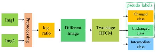
Figure 1.
Generation of pseudo-labels of multi-temporal SAR images.
The next step is to pre-classify the generated DI . In theory, any clustering approach can be employed to cluster the DI into the changed and unchanged classes. Nevertheless, to obtain high-probability changed and high-probability unchanged classes, an effective clustering algorithm should acquire superior intra-class similarity and inter-class difference. Because of the overlap of the changed and unchanged classes, a single partitioned clustering approach, such as FCM, k-means, or their variants, has limited capability and effectiveness in achieving reliable clustering. To overcome the problem and achieve high-probability changed and high-probability unchanged classes, we use the two-stage hierarchical FCM (HFCM) clustering method [30] to cluster the generated into three classes: high-probability changed class (), high-probability unchanged class (), and intermediate class (). The intermediate class () denotes the pixels that are difficult to distinguish by the clustering algorithm. The pixels in and are then chosen as the labels in the training process.
The procedure for clustering into three classes using HFCM algorithm is as follows:
- (1)
- Use the FCM algorithm to cluster the into two clusters: changed cluster () and unchanged cluster (). The number of pixels in the changed cluster () is denoted as . The upper bound of the change class is set as .
- (2)
- Use the FCM algorithm to cluster into five clusters: , , , , and . The five clusters are sorted in descending order by the mean value of each cluster. The cluster with a larger mean value has a higher probability to be changed and vice versa. The number of pixels in the five clusters are denoted as , , , , and , respectively. The pixels in were assigned to the changed class . Set parameters .
- (3)
- Set .
- (4)
- If , assign the pixels in to the intermediate class . Otherwise, the pixels in should be assigned to the unchanged class . Go to step 3 and continue until .
In this way, we can obtain the pseudo labels set [].
The parameter is used to control the number of the intermediate class . For a given DI, when the change class is first determined, the setting of determines the allocation of the number of the intermediate class and unchanged class . If is large, the number of pixels in the intermediate class will be large, and the number of pixels in the unchanged class will be small and vice versa. If the is set too small, the number of pixels in the intermediate class will be very small, and some pixels that are difficult to distinguish by the clustering algorithm will be allocated to the set of unchanged class . It will cause that pixels in the low-probability unchanged class may be selected in the training set. On the contrary, if the is set too large, the number of pixels in the unchanged class will become small. It may cause that we cannot select sufficient unchanged samples. To balance the number of pixels in the unchanged class and intermediate class , is set 1.25.
2.2. Overview of Pyramidal Convolutional Block Attention Network
The architecture of PCBA-Net is illustrated in Figure 2. It is mainly composed of four pyramidal convolutional block attention (PCBA) modules. Every PCBA module consists of a PyConv and a CBAM. First, image patches (with size ) centered at pixels in and and their corresponding pseudo-labels are randomly selected as the training samples. The number of training samples is 10% of the number of pixels in the whole image. The ratio of changed samples to unchanged samples is about 1:1. These training samples are then fed into a convolution with a kernel size of 1 × 1 to generate new feature maps. These feature maps are sequentially forwarded to four PCBA modules to produce representative feature maps. These representative feature maps are then processed by a fully convolutional layer, two linear layers, and a softmax layer to get the final output. After that, a trained model will be obtained. Finally, the trained model is employed to test all patch-pairs in the whole image to generate the final binary CM.
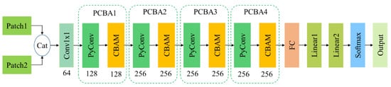
Figure 2.
The architecture of the proposed pyramidal convolutional block attention network (PCBA-Net).
2.3. Pyramidal Convolutional Block Attention Module
The PCBA module is the main component of PCBA-Net. The architecture of PCBA is illustrated in Figure 3. It consists of a PyConv and a CBAM. The PCBA and CBAM are described in detail in the following sections.
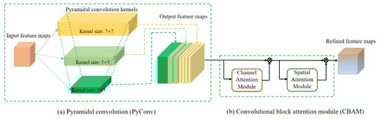
Figure 3.
Sketch of PCBA architecture.
2.3.1. The PyConv Block
Traditional CNN generally utilizes a small and single convolution kernel, which has relatively diminutive receptive field. It cannot acquire enough context information and some other useful detailed information. This causes the network cannot fully extract the feature representation of the input image and adversely affects the recognition performance of the network.
In contrast to traditional convolution, PyConv consists of different levels of kernels, and each level contains diverse types of filters with various sizes and depths. In the implementation of this study, the PyConv contains three levels of different types of convolution kernels, and the structure of these convolution kernels is a inverted pyramid. The kernel sizes increase from the first level (bottom of the pyramid) to the third level (top of the pyramid). As shown in Figure 3a, the kernel sizes of the three levels are 3 × 3, 5 × 5, and 7 × 7, respectively.
Furthermore, the depth of the kernel decreases from the first level to the third level. In order to use different kernel depths at each level of PyConv, the input feature maps are divided into different groups, and each group applies independent kernels. This method is called grouped convolution [36]. We use two examples to explain the grouped convolution. There are four input feature maps in every example. The examples are illustrated in Figure 4. Figure 4a describes the standard convolution, which only includes a single group of input feature maps. In this case, the depth of convolution kernels equals the number of input feature maps. The number of convolution kernels equals the number of output feature maps. Every output feature map connects to every input feature map. Figure 4b illustrates the case that the input feature maps are split into two groups (groups in the example). In this case, each group applies independent kernels, and the depth of convolution kernels in each group becomes 1/2 of the number of input feature maps. The number of convolution kernels in each group is 1/2 of the number of output feature maps. The number of output feature maps in each group is also 1/2 of the number of output feature maps of the whole convolution. As illustrated in Figure 4, when the number of groups increases, the depth of the kernels decreases. As a result, the computational cost of convolution and the number of parameters is reduced by a factor equal to the number of groups. Model parameters and computational costs are described in detail in the next subsection.
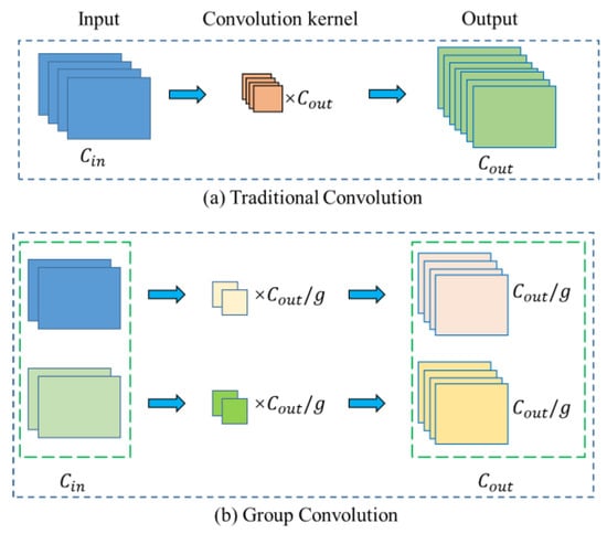
Figure 4.
Grouped Convolution. , , and denote the number of input feature maps, the number of output feature maps, and the number of groups, respectively. in the example.
In the specific implementation of PyConv in this study, the ratio of the number of input feature maps in three convolution levels is 1:1:2, and the group number of grouped convolution is 1, 4, and 8, respectively. Therefore, the ratio of depth of the kernels in the three levels is 4:1:1.
The different types of convolution kernels with incremental kernel sizes can not only expand the receptive field of input features to acquire enough context information, but they also use multi-scaled convolution kernels to handle the input features in parallel. Kernels of smaller size can concentrate on the detail information of smaller objects or parts of objects, while kernels of larger size can focus on the detail information of larger objects and context information. In this way, the multi-scaled convolution kernels in PyConv can obtain complementary information and enhance the recognition performance of the network.
2.3.2. Model Parameters and Floating-Point Operations (FLOPs) of PyConv
Model parameters and floating-point operations (FLOPs) are two important indicators of network model complexity [36]. For the standard convolution, the number of parameters and FLOPs are calculated as follows:
For the grouped convolution, the number of parameters and FLOPs are expressed as:
where and denote the number of input feature maps and the number of output feature maps, respectively. The convolution kernel size is . and indicate the height and width of the input feature maps, respectively. represents the number of groups in grouped convolution.
For the proposed PyConv, the number of parameters and FLOPs are expressed as:
where , , and denote the number of input feature maps in the first level, the second level, and the third level of PyConv, respectively. , , and represent the number of output feature maps in the first level, the second level, and the third level of PyConv, respectively. , , and refer to the number of groups that the input feature maps are divided in the first level, the second level, and the third level of PyConv, respectively. , , and denote the convolution kernel sizes of the first level, the second level, and the third level of PyConv, respectively. denotes the number of output feature maps of PyConv. and indicate the height and width of the input feature maps, respectively.
2.3.3. Convolutional Block Attention Module
CBAM is another crucial component of PCBA. As Figure 3b shown, CBAM comprises two parts: channel attention and spatial attention [38]. For a given input feature map F with size C × H × W, CBAM generates a 1D channel attention map with size C × 1 × 1 and a 2D spatial attention map with size 1 × H × W, sequentially. This process is depicted in Figure 3b, which can be represented by following Equation:
where denotes element-wise multiplication.
In the channel attention model, average pooling and max pooling are first performed on the input feature map F to acquire two feature vectors (e.g., average-pooled features and max-pooled features) with size C × 1 × 1, respectively. Then, the two feature vectors are respectively processed by a weight-sharing multi-layer perceptron (MLP) with one hidden layer. After that, the two feature vectors are merged into one with element-wise summation, and a sigmoid function σ is employed on it to obtain channel attention map . In brief, channel attention is expressed as:
where σ represents the sigmoid function, and are the MLP weights, and their dimensions are C/r × C and C × C/r, respectively. r denotes the reduction ratio.
In the spatial attention module, average pooling and max pooling are also performed on the feature map F to generate two 2D maps. The two 2D maps are then concatenated and processed by a standard convolution layer. In brief, spatial attention is expressed as:
where σ indicates the sigmoid function and represents a convolution operation with the filter size of .
3. Experimental Results
In this section, we first introduce the experimental dataset and evaluation criteria. The experimental setup is then described. Finally, experimental results and comparison with other methods are presented.
3.1. Dataset
In this study, six actual multi-temporal SAR datasets are used to assess the proposed approach. The ground truth of change maps is annotated by experts by integrating prior information and photo interpretation. Raw images of the six datasets and their ground truth are shown in Figure 5, Figure 6, Figure 7, Figure 8, Figure 9 and Figure 10, respectively.
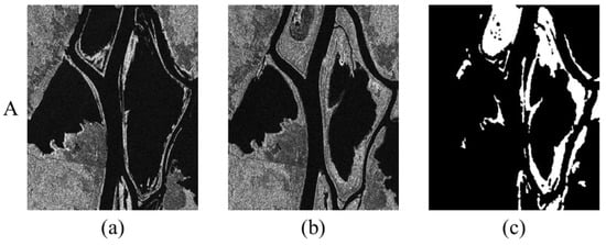
Figure 5.
Ottawa dataset. (a) Image acquired in July 1997. (b) Image acquired in August 1997. (c) Ground-truth map.
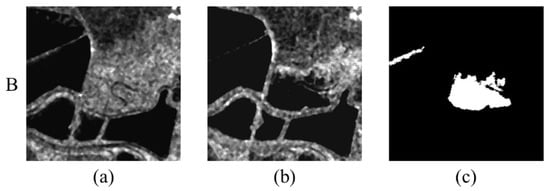
Figure 6.
San Francisco dataset. (a) Image acquired in August 2003. (b) Image acquired in May 2004. (c) Ground-truth map.
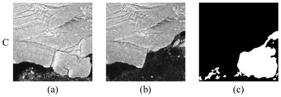
Figure 7.
Sulzberger dataset. (a) Image acquired on 11 March 2011. (b) Image acquired on 16 March 2011. (c) Ground-truth map.
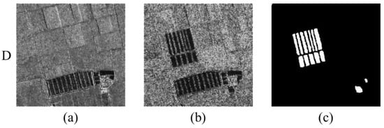
Figure 8.
Yellow River A Dataset. (a) Image acquired in June 2008. (b) Image acquired in June 2009. (c) Ground-truth map.
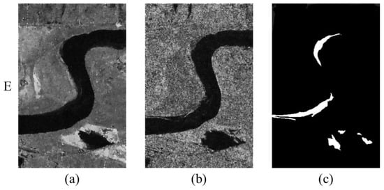
Figure 9.
Yellow River B Dataset. (a) Image acquired in June 2008. (b) Image acquired in June 2009. (c) Ground-truth map.
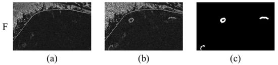
Figure 10.
Yellow River C Dataset. (a) Image acquired in June 2008. (b) Image acquired in June 2009. (c) Ground-truth map.
The first dataset (recorded as Dataset A) is the Ottawa dataset (as Figure 5 shown). This pair of images was acquired by the RADARSAT satellite in July and August 1997. This dataset showed the changes caused by floods in Ottawa, and it was provided by the National Defense Research and Development Canada. Its size is 290 × 350 pixels, and its spatial resolution is 10 m.
The second dataset (recorded as Dataset B) is the San Francisco dataset with the spatial resolution of 30 m (as Figure 6 shown). It was captured by the ERS-2 SAR sensor in August 2003 and May 2004. The original size of the image is 7749 × 7713 pixels. As the original image is too large to show the detailed information, a typical region with size of 256 × 256 pixels is chosen in this study.
The third dataset (recorded as Dataset C) is the Sulzberger dataset (shown in Figure 7). It was obtained by the European Space Agency’s ENVISAT satellite on March 11 and 16, 2011. It was captured from a large SAR image in the region of the Sulzberger Ice Shelf. The Sulzberger Ice Shelf was flexed and broken when the Tohoku Tsunami was triggered in the Pacific Ocean on 11 March 2011. The images reflect the progression of ice breakup. The size of original SAR images is 2263 × 2264 pixels. Because the original image is too large to display the detailed information, a typical area with size of 256 × 256 pixels is chosen in this study.
The last three datasets (recorded as Dataset D, Dataset E, and Dataset F, respectively) were captured from the Yellow River dataset (as shown in Figure 8, Figure 9 and Figure 10). The Yellow River dataset was acquired by the Radarsat-2 satellite in June 2008 and June 2009. Its spatial resolution is 8 m. The images display changes in the region of Yellow River estuary from 2008 to 2009. Particularly, one image of the dataset is a single-look image while the other is a four-look image. This dataset is polluted by noise of different characteristics, which makes it very challenging to perform CD on this dataset. The size of the original image is 7666 × 7692 pixels. As the size of the original image is too large to represent detailed information, three representative regions are selected in the experiment. We call them Yellow River A dataset, Yellow River B dataset, and Yellow River C dataset. The corresponding sizes of the three datasets are 306 × 291, 291 × 444, and 450 × 280, respectively.
3.2. Evaluation Criteria
To evaluate the performance of the proposed CD method, we assign the changed pixels as positive and the unchanged pixels as negative. A confusion matrix is then constructed. True positive (TP) represents the number of changed pixels correctly detected; true negative (TN) refers the number of unchanged pixels correctly detected; false positive (FP) indicates the number of unchanged pixels detected as the changed ones; and false negative (FN) denotes the number of changed pixels detected as the unchanged ones.
Six qualitative indicators, i.e., FP, FN, overall error (OE), percentage of correct classification (PCC), kappa coefficient (KC), and F1 score (F1), are employed in the experiments.
OE indicates the total number of errors and it is calculated as the sum of FN and FP. OE is expressed as:
PCC denotes the correct rate of the classification, and it is calculated as follows:
KC is a measure of accuracy or agreement based on the difference between the error matrix and the change agreement [40]. KC is expressed as follows:
where
F1 score is the harmonic mean of the precision and recall, which can be calculated as:
3.3. Experimental Setup
The structure of the proposed PCBA-Net is illustrated in Figure 2. PCBA-Net consists of a convolution with a kernel size of 1 × 1 (Conv1 × 1), four PCBA models, a fully convolutional layer, two linear layers, and a softmax layer. The PCBA model includes a PyConv and a CBAM. Batchnorm is used in the PyConv layers. There are three different convolution kernels in the PyConv, and these kernel sizes are 3 × 3, 5 × 5, and 7 × 7, respectively. The parameters of every layer in PCBA-Net are listed in Table 1. ReLU is used as the activation function in PyConv layers. Epoch number, batch size, and learning rate are set to 50, 1024, and 0.001, respectively. All of the experiments are conducted on a desktop computer with a 3.3 GHz four-core CPU, a 32 GB RAM, and a NVIDIA GeForce RTX 3090 GPU with 24 GB memory.

Table 1.
The parameters of every layer in PCBA-Net.
3.4. Experimental Results and Comparison
In this subsection, we present the results of the proposed PCBA-Net. To demonstrate the effectiveness of our method, we compare our results with several state-of-the-art approaches, including PCANet [30], the CNN method [13], CWNN [31], DDNet [14], and SAFNet [32]. The best results are shown in bold.
3.4.1. Results of the Ottawa Dataset
The change map of Ottawa dataset is depicted in Figure 11, while the quantitative metrics for CD are shown in Table 2. From Figure 11, we can see that the PCANet method ignores many changed areas, especially in the red and green rectangle areas. Therefore, it has the biggest FN value. For the CNN method, it improperly detects many unchanged pixels as the changed ones, especially in the blue rectangle area. As a result, it has the largest FP value. CWNN also incorrectly detects numerous unchanged pixels as the changed ones, especially in the upper part of the red rectangular area. It also loses many image details. The DDNet method also mistakenly detects a lot of unchanged pixels as the changed ones. Its FP value is also quite large. Both the FP and FN values of SAFNet are unremarkable. The proposed PCBA-Net preserves the details of the change area and attains the best CD performance. In terms of quantitative metrics, the FP, OE, PCC, KC, and F1 score of our proposed PCBA-Net exceed the results of the five compared methods. As shown in Table 2, the PCC of the proposed PCBA-Net increases by 0.73%, 0.96%, 0.45%, 0.69%, and 0.7% over PCANet, CNN, CWNN, DDNet, and SAFNet, respectively. Moreover, the KC of the proposed PCBA-Net is improved by 2.71%, 3.36%, 1.5%, 2.41%, and 2.58% over the five compared methods, respectively. Furthermore, compared with the five compared methods, the F1 score increases by 2.27%, 2.78%, 1.22%, 1.99%, and 2.16%, respectively.
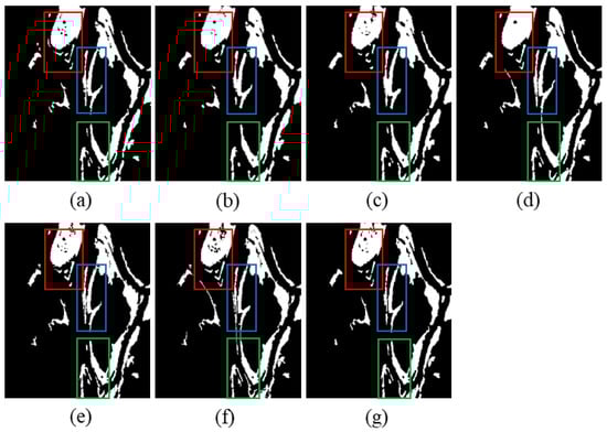
Figure 11.
Visualization of comparative experimental results for the Ottawa dataset. (a) Ground-truth image. (b) Result of PCANet. (c) Result of CNN. (d) Result of CWNN. (e) Result of DDNet. (f) Result of SAFNet. (g) Result of the presented PCBA-Net.
Table 2.
Change detection results for Ottawa dataset.
3.4.2. Results for the San Francisco Dataset
The change map for the San Francisco dataset is illustrated in Figure 12, and the quantitative evaluation is listed in Table 3. Figure 12 reveals that both the PCANet and CNN methods neglect a large number of changed pixels, especially in the red rectangle region. Consequently, these two methods have large FN values. The CWNN method detects hundreds of unchanged pixels as the changed ones. This results in CWNN having the largest FP value. Furthermore, there are three isolated false alarm areas in its change map. For the DDNet method, neither the FP nor FN value is prominent. Moreover, there are also three isolated incorrect detection areas in its change map. Although SAFNet has a small FP value, its FN value is quite large. In other words, it ignores numerous changed pixels and loses many details. Although there are also two isolated incorrect detection areas in the change map of our PCBA-Net, it preserves the details of the change area, especially in the red rectangle region. In terms of quantitative evaluation, the OE, PCC, KC, and F1 score of our proposed PCBA-Net outperform the results of the five compared methods. As shown in Table 3, compared with the five other methods, the PCC of our proposed PCBA-Net obtains an increase of 0.34%, 0.42%, 0.34%, 0.28%, and 0.19%, respectively. Meanwhile, the KC of our method improves by 2.76%, 3.34%, 2.29%, 2.14%, and 1.61%, respectively. Additionally, the F1 score also increases by 2.58%, 3.12%, 2.11%, 1.99%, and 1.51%, respectively.
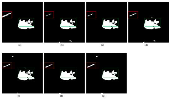
Figure 12.
Visualization of comparative experiments for the San Francisco dataset. (a) Ground-truth image. (b) Result of PCANet. (c) Result of CNN. (d) Result of CWNN. (e) Result of DDNet. (f) Result of SAFNet. (g) Result of the presented PCBA-Net.
Table 3.
Change detection results for San Francisco dataset.
3.4.3. Results for the Sulzberger Dataset
For the Sulzberger dataset, the change map is described in Figure 13, and quantitative metrics for CD are given in Table 4. From Figure 13, it can be seen that the CNN method incorrectly detects numerous unchanged pixels as the changed ones, especially in the red rectangle zone. Accordingly, it has the largest FP values. Furthermore, CWNN also falsely detects a large number of unchanged pixels as the changed ones. On the contrary, SAFNet ignores a lot of changed pixels, especially in the red rectangle area. As a result, it has the largest FN values. Moreover, DDNet also neglects hundreds of changed pixels. Both the SAFNet and DDNet methods lose much detailed information in the change maps. PCANet acquires better CD performance than the abovementioned methods, but it still has quite a large FN value. Our PCBA-Net achieves the best detection results. In terms of quantitative metrics, the OE, PCC, KC, and F1 score of our proposed PCBA-Net surpass the results of PCANet, CNN, CWNN, DDNet, and SAFNet methods. The PCC of our proposed PCBA-Net improves by 0.24%, 1.18%, 0.52%, 0.6%, and 0.58% over the five compared approaches, respectively. The KC of our method increases by 0.81%, 3.71%, 1.58%, 1.99%, and 1.97% over the five compared approaches, respectively. The F1 score of our approach increases by 0.66%, 2.97%, 1.26%, 1.62%, and 1.62% over the five compared approaches, respectively.
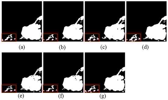
Figure 13.
Visualization of comparative experiments for the Sulzberger dataset. (a) Ground-truth image. (b) Result of PCANet. (c) Result of CNN. (d) Result of CWNN. (e) Result of DDNet. (f) Result of SAFNet. (g) Result of the presented PCBA-Net.
Table 4.
Change detection results for Sulzberger dataset.
3.4.4. Results for the Yellow River Datasets
The change maps of the Yellow River datasets are illustrated in Figure 14, Figure 15 and Figure 16, and the corresponding quantitative metrics for CD are shown in Table 5, Table 6 and Table 7. As the Yellow River datasets contain a wealth of speckle noise, it is highly challenging to detect changes in the datasets.
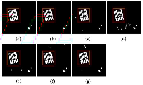
Figure 14.
Visualization of comparative experiments for the Yellow River A dataset. (a) Ground-truth image. (b) Result of PCANet. (c) Result of CNN. (d) Result of CWNN. (e) Result of DDNet. (f) Result of SAFNet. (g) Result of the presented PCBA-Net.
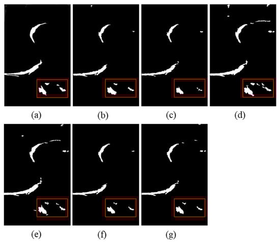
Figure 15.
Visualization of comparative experiments for the Yellow River B dataset. (a) Ground-truth image. (b) Result of PCANet. (c) Result of CNN. (d) Result of CWNN. (e) Result of DDNet. (f) Result of SAFNet. (g) Result of the presented PCBA-Net.
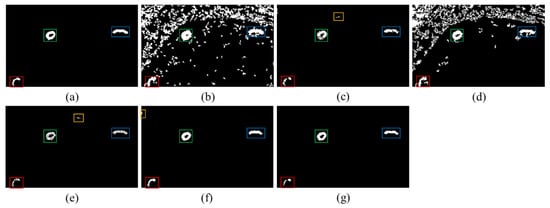
Figure 16.
Visualization of comparative experiments for the Yellow River C dataset. (a) Ground-truth image. (b) Result of PCANet. (c) Result of CNN. (d) Result of CWNN. (e) Result of DDNet. (f) Result of SAFNet. (g) Result of the presented PCBA-Net.
Table 5.
Change detection results for Yellow River A dataset.
Table 6.
Change detection results for Yellow River B dataset.
Table 7.
Change detection results for Yellow River C dataset.
For the Yellow River A dataset, as shown in Figure 14, the CNN method neglects thousands of changed pixels and it causes the change map edge not smooth. Consequently, it has the largest FN values. A more serious problem is that it improperly detects hundreds of unchanged pixels as the changed ones, which causes it to have the largest FP value. PCANet also ignores numerous changed pixels. It has a very high FN value as well. This leads to PCANet missing a lot of detailed information, especially in the red rectangle area. CWNN incorrectly detects a large number of unchanged pixels as the changed ones. It causes some incorrect insular change areas under the red rectangle in the change map. Although DDNet and SAFNet have better detection performance, there are still some incorrect isolated change areas in the corresponding change maps. Furthermore, these two approaches also lose much detailed information, especially in the red rectangle areas. The proposed PCBA-Net method acquires the best detection performance. Although it also incorrectly detects some unchanged pixels as the changed ones and causes two false isolated change areas in the change map, it preserves the details of change information to the utmost extent, especially in the red rectangle area. In terms of quantitative metrics, as shown in Table 5, the OE, PCC, KC, and F1 score of our method are better than the results of the five comparative methods. Compared with the five other algorithms, the PCC of our approach increases by 0.33%, 1.07%, 0.39%, 0.21%, and 0.27%, respectively. The KC increases by 3.86%, 10.72%, 3.45%, 2.29%, and 2.9% over the five compared approaches, respectively. Furthermore, the F1 score improves by 3.71%, 10.17%, 3.25%, 2.19%, and 2.76% over the five compared approaches, respectively.
For the Yellow River B dataset, as shown in Figure 15, the CWNN method detects many unchanged pixels as the changed ones. Therefore, it has the largest FP value. It also causes some false alarm areas in the change map. On the contrary, the CNN method suffers from the largest FN value and ignores many changed pixels, especially in the red rectangle area. Similarly, PCANet and SAFNet also neglect numerous changed pixels and have large FN values. Although DDNet has a small FN value, its FP value is quite large. Our PCBA-Net achieves outstanding performance. In terms of quantitative metrics, as shown in Table 6, the OE and PCC of our PCBA-Net surpass all five comparative approaches. The PCC of our method increases by 0.22%, 0.11%, 0.39%, 0.02%, and 0.07% in comparison with the five other approaches, respectively. Compared with PCANet, CNN, CWNN, and SAFNet approaches, the KC improves by 4.27%, 3.19%, 2.88%, and 2.39%, and the F1 score increases by 4.17%, 3.15%, 2.69%, and 2.37%, respectively. Although the KC and F1 score of our PCBA-Net are lower than the corresponding values of DDNet, the OE and PCC of our PCBA-Net outperform the corresponding values of DDNet.
For the Yellow River C dataset, as depicted in Figure 16, both the PCANet and CWNN methods falsely detect numerous unchanged pixels as the changed ones. This causes both the PCANet and CWNN methods to have very large FP values. The CNN and DDNet methods neglect hundreds of changed pixels, especially in the red, green, and blue rectangle regions. Additionally, these two methods incorrectly detect hundreds of unchanged pixels as the changed ones, especially in the orange rectangle zone. SAFNet obtains better CD performance than the abovementioned methods, but it still mistakenly detects hundreds of unchanged pixels as the changed ones, especially in the orange rectangle region. The proposed PCBA-Net acquires the best CD performance and preserves the detail information of the change areas. In terms of quantitative metrics, the FP, OE, PCC, KC, and F1 score of our proposed PCBA-Net surpass the results of the five compared methods. As shown in Table 7, the PCC of our PCBA-Net increases by 13.53%, 0.26%, 10.29%, 0.22%, and 0.03% compared with the five other methods, respectively. Meanwhile, the KC of our PCBA-Net improves by 76%, 11.83%, 72.98%, 12.6%, and 0.76% over the five compared approaches, respectively. Moreover, the F1 score of our PCBA-Net increases by 74.37%, 11.7%, 71.44%, 12.51%, and 0.76%, respectively.
4. Discussion
In this study, PCBA-Net is proposed for SAR image CD. We use PyConv to learn appropriate feature representation. In order to accentuate the momentous features, CBAM is introduced in the proposed PCBA-Net. Six actual datasets are utilized to assess the performance of PCBA-Net in the experiments. FP, FN, OE, PCC, KC, and F1 score are used as evaluation parameters to assess the CD results. The results of six real SAR datasets confirm the effectiveness of our proposed method. The proposed PCBA-Net outperforms several state-of-the-art methods.
In our PCBA-Net, PyConv is utilized to extract the features of multi-temporal SAR images. The PyConv in our module contains three levels of different convolution kernels of diverse sizes and depths. PyConv can expand the receptive field of the input features. Moreover, it can manage the input feature with incremental convolution kernel sizes in parallel to acquire multi-scale detailed information. Concretely, kernels of smaller size have tiny receptive fields and concentrate on capturing information regarding smaller objects and parts of objects. Conversely, kernels of larger size have large receptive fields and center on acquiring detailed information regarding larger objects and context information. As a result, PyConv can capture complementary information and improve the recognition performance of the network. Furthermore, grouped convolution is used in the PyConv. This helps PyConv to use kernels with different depths and to reduce the computational cost. Compared with standard convolution, PyConv sustains a similar number of model parameters and computational resource requirements. The main contributions of this study can be summarized as follows:
(1) PyConv is introduced for SAR image CD. PyConv can not only extend the receptive field of input to capture enough context information, but it also handles the input with incremental kernel sizes in parallel to obtain multi-scale detailed information of SAR images.
(2) CBAM is embedded into the PyConv to emphasize vital features of SAR images. CBAM can enhance crucial features and restrain redundant features in the channel and spatial axes of SAR images.
In the experiments, we compare the proposed PCBA-Net with the PCANet [30], CNN [13], CWNN [31], DDNet [14], and SAFNet [32] methods. Details of compared results are described in Section 3.4. In PCANet, Gabor wavelets and FCM are used to obtain the pre-classified samples as the labeled samples, and PCANet is utilized for extracting features and classification. PCANet uses PCA filters as convolutional filters. On five datasets, PCANet has quite high FN values. This means that PCANet ignores a large number of changed pixels and misses much detailed information. In the CNN method, a spatial fuzzy clustering algorithm is used to pre-classify the DI for acquiring pseudo-labels. CNN with two convolution layers and two pooling layers is used for extracting features and classification. Because the structure of the CNN method is extremely simple, its capacity for feature extraction is quite weak. This causes unsatisfactory results for CD. In CWNN, dual-tree complex wavelet transform (DT-CWT) is introduced to CNN to alleviate the infection of speckle noise. CWNN has a small FN value, but its FP value is quite large. This means that numerous unchanged pixels are incorrectly detected as the changed pixels. In DDNet, a multi-region convolution (MRC) module is proposed, and features in discrete cosine transform (DCT) domain are integrated into the CNN model. In this way, both spatial and frequency features can be exploited in the DDNet method. In SAFNet, a siamese neural network is presented to extract features of multi-temporal SAR images, and an adaptive fusion module is used to compound multi-scaled features in different convolutional layers. A correlation layer is utilized to exploit the correlation between multi-temporal images. Although DDNet and SAFNet improve the performance of SAR image CD to some extent, the CD results remain unsatisfactory. Compared with the above methods, the proposed PCBA-Net obtains the best CD performance in the six actual datasets.
Moreover, we also compare the model parameters, FLOPs, training time, and testing time of the proposed PCBA-Net with four CNN-based approaches, i.e., CNN, CWNN, DDNet, and SAFNet (as shown in Table 8). Because PCANet is not a CNN-based method, it is inappropriate to compare its parameters and model complexity with CNN-based methods. Thus, we do not list these parameters of PCANet. The training time and test time are calculated on computer with NVIDIA GeForce RTX 3090 GPU with 24 GB memory when the batch size is equal to 1024. Table 8 lists these four parameters. According to Table 8, the FLOPs, training time, and testing time of the proposed PCBA-Net are larger than the four compared CNN-based methods. Although the proposed PCBA-Net has the largest parameters and FLOPs compared with the four CNN-based methods, its model parameters were only 1.873 M, which is not too large. Furthermore, we notice that CWNN has fewer parameters and FLOPs than DDNet and SAFNet (as shown in Table 8), but the performance of CWNN surpasses the performance of DDNet and SAFNet in the Ottawa and Sulzberger datasets (as shown in Table 2 and Table 3, respectively). DDNet has fewer parameters and FLOPs than SAFNet (as shown in Table 8), but the performance of DDNet exceeds the performance of SAFNet in the Ottawa, Yellow River A, and Yellow River B datasets (as shown in Table 2, Table 5, and Table 6, respectively). CNN has fewer parameters and FLOPs than CWNN (as shown in Table 8), but the performance of the CNN method is superior to the performance of CWNN in the Yellow River B and Yellow River C datasets (as shown in Table 6 and Table 7, respectively). This means that the performance of networks does not increase strictly with the increase of the model parameters and FLOPs. In addition, we also observe that DDNet has fewer parameters and FLOPs than SAFNet, but it has larger training and testing times than SAFNet (as shown in Table 8). This means that the training and testing time of networks also does not increase strictly with the increase of the model parameters and FLOPs.
Table 8.
The parameters, FLOPs, training time, and testing time of the proposed PCBA-Net and four CNN-based approaches.
In PyConv, the number of levels and convolution kernel size are important parameters. These parameters may impact feature extraction and affect the performance of CD. Hence, we investigate the effects of these parameters on CD performance. Diverse kernel sizes and levels are designed in the experiments, as shown in the first column of Table 9. PCC is used as the evaluation parameter to indicate the performance of CD in the experiments. PCC values with different types of PyConv are listed in Table 9. The best results are shown in bold. According to Table 9, the PyConv with kernels of 3 × 3, 5 × 5, and 7 × 7 obtains the best results in the six real datasets. This confirms that the PyConv with multi-scale convolution kernels can improve the recognition performance of the network.
Table 9.
PCC value [%] of the six datasets with different types of pyramidal convolution.
For the PCBA-Net, the number of PCBA blocks may have an effect on the performance of SAR image CD. Therefore, we research the relationship between PCC values and the number of PCBA blocks. We set the number of PCBA block to 1, 2, 3, 4, and 5. Figure 17 depicts the PCC values with different numbers of the PCBA blocks on the six datasets. According to Figure 17, PCC values increase with increasing number of PCBA blocks at first. PCC values reach their maximum when the number of PCBA blocks is 4, then PCC values start to decrease. This may be because the PCBA-Net model is relatively simple and cannot extract the features of SAR images sufficiently when the number of PCBA blocks is less than 4. The capability of feature extraction of the proposed PCBA-Net grows with the increase in the number of PCBA blocks. PCBA-Net has the highest ability to extract features when the number of PCBA blocks is equal to 4. With a continued increase in the number of PCBA blocks, the parameters and model complexity of PCBA-Net increase, which causes over-fitting of the network. Therefore, we use four PCBA blocks in the PCBA-Net.
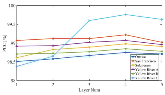
Figure 17.
The PCC values with different numbers of PCBA blocks.
Furthermore, spatial context information is related to the size of input patch-pairs. The size of input patch-pairs is denoted as r × r × 2. The value of r may influence the CD performance of PCBA-Net. Accordingly, we explore the relationship between r and PCC. We set r = 5, 7, 9, 11, 13, 15, 17, 19, and 21 in the experiments. Then we use sample patch-pairs with these sizes of r to train the PCBA-Net. Figure 18 shows the PCC values with different values of r on the six datasets. The PCC values increase and then tend to be stable with the increment of r values. When r = 7, PCC values reach the maximum for all six datasets. This indicates that it is difficult to identify changed information of the center pixel using large patch size. Additionally, the larger patch size increases the complexity and computation cost of the model, resulting in a decrease in model performance. After comprehensive consideration, we set r = 7 in the experiments.
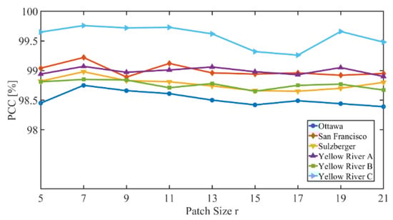
Figure 18.
The PCC value with different values of r.
In addition, in order to explore the effectiveness of the PCBA-Net module, ablation experiments are conducted on the six datasets. CNN refers to the traditional CNN network, which has the same number of layers and output shape as PyConv in the PCBA-Net. The performance of CD is evaluated by PCC. The results of the ablation study are listed in Table 10. The best results are shown in bold. The PyConv model outperforms the CNN model (PCC values in the third row vs. PCC values in the first row). This demonstrates that the PyConv can enhance the recognition performance of the network. Moreover, when the CBAM is introduced to the network, the performance model also improves (PCC values in the fourth row vs. PCC values in the third row). This indicates that both PyConv and CBAM play important roles in improving the results of CD. Removing either the Pyconv model or the CBAM module will reduce the performance of CD.
Table 10.
PCC value [%] of the six datasets in ablation study of the proposed PCBA-Net.
5. Conclusions
In this study, we propose a novel PCBA-Net to implement CD on SAR images. In PCBA-Net, PyConv is utilized to enlarge the receptive field of input features to capture enough context information and to handle input features with incremental kernel sizes in parallel to obtain multi-scale detailed information of SAR images. In order to emphasize crucial features and suppress unnecessary features in the channel and spatial axes, CBAM is adopted in the proposed PCBA-Net. Six actual SAR datasets are used to evaluate the performance of PCBA-Net. Compared with several state-of-the-art algorithms, the results of PCBA-Net in six actual SAR datasets manifest that the PCBA-Net achieves superior performance in CD. In the future, we will research CD on heterogeneous images.
Author Contributions
Conceptualization, Y.X. and X.X.; Methodology, Y.X. and X.X.; Software, Y.X.; Data curation, Y.X.; Writing—Original draft preparation, Y.X.; Visualization, Y.X.; Investigation, Y.X.; Supervision, X.X.; Resources, X.X.; Validation, X.X. and F.P.; Writing—Reviewing and Editing, X.X. and F.P. All authors have read and agreed to the published version of the manuscript.
Funding
This work was supported by the National Natural Science Foundation of China under Grant 62071336.
Data Availability Statement
Not applicable.
Conflicts of Interest
The authors declare no conflict of interest.
References
- Radke, R.J.; Andra, S.; Al-Kofahi, O.; Roysam, B. Image change detection algorithms: A systematic survey. IEEE Trans. Image Process. 2005, 14, 294–307. [Google Scholar]
- Gong, M.; Yang, H.; Zhang, P. Feature learning and change feature classification based on deep learning for ternary change detection in SAR images. ISPRS J. Photogramm. Remote Sens. 2017, 129, 212–225. [Google Scholar] [CrossRef]
- Zhang, H.; Liu, W.; Shi, J.; Fei, T.; Zong, B. Joint detection threshold optimization and illumination time allocation strategy for cognitive tracking in a networked radar system. IEEE Trans. Signal Process. 2022. [Google Scholar] [CrossRef]
- Liang, X.; Chen, B.; Chen, W.; Wang, P.; Liu, H. Unsupervised Radar Target Detection under Complex Clutter Background Based on Mixture Variational Autoencoder. Remote Sens. 2022, 14, 4449. [Google Scholar]
- Brunner, D.; Lemoine, G.; Bruzzone, L. Earthquake damage assessment of buildings using VHR optical and SAR imagery. IEEE Trans. Geosci. Remote Sens. 2010, 48, 2403–2420. [Google Scholar] [CrossRef]
- Yousif, O.; Ban, Y. Improving SAR-based urban change detection by combining MAP-MRF classifier and nonlocal means similarity weights. IEEE J. Sel. Top. Appl. Earth Obs. Remote Sens. 2014, 7, 4288–4300. [Google Scholar] [CrossRef]
- Lunetta, R.S.; Knight, J.F.; Ediriwickrema, J.; Lyon, J.G.; Worthy, L.D. Land-cover change detection using multi-temporal MODIS NDVI data. Remote Sens. Environ. 2006, 105, 142–154. [Google Scholar] [CrossRef]
- Pantze, A.; Santoro, M.; Fransson, J.E. Change detection of boreal forest using bi-temporal ALOS PALSAR backscatter data. Remote Sens. Environ. 2014, 155, 120–128. [Google Scholar]
- Li, Y.; Gong, M.; Jiao, L.; Li, L.; Stolkin, R. Change-detection map learning using matching pursuit. IEEE Trans. Geosci. Remote Sens. 2015, 53, 4712–4723. [Google Scholar] [CrossRef]
- Yuan, Y.; Lv, H.; Lu, X. Semi-supervised change detection method for multi-temporal hyperspectral images. Neurocomputing 2015, 148, 363–375. [Google Scholar] [CrossRef]
- Moser, G.; Serpico, S.B. Unsupervised change detection from multichannel SAR data by Markovian data fusion. IEEE Trans. Geosci. Remote Sens. 2009, 47, 2114–2128. [Google Scholar] [CrossRef]
- Bruzzone, L.; Prieto, D.F. An adaptive semiparametric and context-based approach to unsupervised change detection in multitemporal remote-sensing images. IEEE Trans. Image Process. 2002, 11, 452–466. [Google Scholar] [CrossRef] [PubMed]
- Li, Y.; Peng, C.; Chen, Y.; Jiao, L.; Zhou, L.; Shang, R. A deep learning method for change detection in synthetic aperture radar images. IEEE Trans. Geosci. Remote Sens. 2019, 57, 5751–5763. [Google Scholar] [CrossRef]
- Qu, X.; Gao, F.; Dong, J.; Du, Q.; Li, H.-C. Change detection in synthetic aperture radar images using a dual-domain network. IEEE Geosci. Remote Sens. Lett. 2021, 19, 1–5. [Google Scholar] [CrossRef]
- Moser, G.; Serpico, S.B. Generalized minimum-error thresholding for unsupervised change detection from SAR amplitude imagery. IEEE Trans. Geosci. Remote Sens. 2006, 44, 2972–2982. [Google Scholar] [CrossRef]
- Bazi, Y.; Bruzzone, L.; Melgani, F. Automatic identification of the number and values of decision thresholds in the log-ratio image for change detection in SAR images. IEEE Geosci. Remote Sens. Lett. 2006, 3, 349–353. [Google Scholar] [CrossRef]
- Inglada, J.; Mercier, G. A new statistical similarity measure for change detection in multitemporal SAR images and its extension to multiscale change analysis. IEEE Trans. Geosci. Remote Sens. 2007, 45, 1432–1445. [Google Scholar] [CrossRef]
- Hou, B.; Wei, Q.; Zheng, Y.; Wang, S. Unsupervised change detection in SAR image based on Gauss-log ratio image fusion and compressed projection. IEEE J. Sel. Top. Appl. Earth Obs. Remote Sens. 2014, 7, 3297–3317. [Google Scholar] [CrossRef]
- Ma, J.; Gong, M.; Zhou, Z. Wavelet fusion on ratio images for change detection in SAR images. IEEE Geosci. Remote Sens. Lett. 2012, 9, 1122–1126. [Google Scholar] [CrossRef]
- Zheng, Y.; Jiao, L.; Liu, H.; Zhang, X.; Hou, B.; Wang, S. Unsupervised saliency-guided SAR image change detection. Pattern Recognit. 2017, 61, 309–326. [Google Scholar] [CrossRef]
- Zhuang, H.; Hao, M.; Deng, K.; Zhang, K.; Wang, X.; Yao, G. Change detection in SAR images via ratio-based gaussian kernel and nonlocal theory. IEEE Trans. Geosci. Remote Sens. 2021, 60, 1–15. [Google Scholar] [CrossRef]
- Sun, Y.; Lei, L.; Li, X.; Tan, X.; Kuang, G. Structure consistency-based graph for unsupervised change detection with homogeneous and heterogeneous remote sensing images. IEEE Trans. Geosci. Remote Sens. 2021, 60, 1–21. [Google Scholar] [CrossRef]
- Kittler, J.; Illingworth, J. Minimum error thresholding. Pattern Recognit. 1986, 19, 41–47. [Google Scholar] [CrossRef]
- Dempster, A.P.; Laird, N.M.; Rubin, D.B. Maximum likelihood from incomplete data via the EM algorithm. J. R. Stat. Soc. Ser. B 1977, 39, 1–22. [Google Scholar]
- Su, L.; Gong, M.; Sun, B.; Jiao, L. Unsupervised change detection in SAR images based on locally fitting model and semi-EM algorithm. Int. J. Remote Sens. 2014, 35, 621–650. [Google Scholar] [CrossRef]
- Celik, T. Unsupervised change detection in satellite images using principal component analysis and $ k $-means clustering. IEEE Geosci. Remote Sens. Lett. 2009, 6, 772–776. [Google Scholar] [CrossRef]
- Gong, M.; Zhou, Z.; Ma, J. Change detection in synthetic aperture radar images based on image fusion and fuzzy clustering. IEEE Trans. Image Process. 2011, 21, 2141–2151. [Google Scholar] [CrossRef]
- Krinidis, S.; Chatzis, V. A robust fuzzy local information C-means clustering algorithm. IEEE Trans. Image Process. 2010, 19, 1328–1337. [Google Scholar]
- Tian, D.; Gong, M. A novel edge-weight based fuzzy clustering method for change detection in SAR images. Inf. Sci. 2018, 467, 415–430. [Google Scholar] [CrossRef]
- Gao, F.; Dong, J.; Li, B.; Xu, Q. Automatic change detection in synthetic aperture radar images based on PCANet. IEEE Geosci. Remote Sens. Lett. 2016, 13, 1792–1796. [Google Scholar] [CrossRef]
- Gao, F.; Wang, X.; Gao, Y.; Dong, J.; Wang, S. Sea ice change detection in SAR images based on convolutional-wavelet neural networks. IEEE Geosci. Remote Sens. Lett. 2019, 16, 1240–1244. [Google Scholar] [CrossRef]
- Gao, Y.; Gao, F.; Dong, J.; Du, Q.; Li, H.-C. Synthetic Aperture Radar Image Change Detection via Siamese Adaptive Fusion Network. IEEE J. Sel. Top. Appl. Earth Obs. Remote Sens. 2021, 14, 10748–10760. [Google Scholar] [CrossRef]
- Liu, F.; Jiao, L.; Tang, X.; Yang, S.; Ma, W.; Hou, B. Local restricted convolutional neural network for change detection in polarimetric SAR images. IEEE Trans. Neural Netw. Learn. Syst. 2018, 30, 818–833. [Google Scholar] [CrossRef] [PubMed]
- Zhao, G.; Peng, Y. Semisupervised SAR image change detection based on a siamese variational autoencoder. Inf. Process. Manag. 2022, 59, 102726. [Google Scholar] [CrossRef]
- Zhou, B.; Khosla, A.; Lapedriza, A.; Oliva, A.; Torralba, A. Object detectors emerge in deep scene cnns. arXiv 2014, arXiv:1412.6856. [Google Scholar]
- Duta, I.C.; Liu, L.; Zhu, F.; Shao, L. Pyramidal convolution: Rethinking convolutional neural networks for visual recognition. arXiv 2020, arXiv:2006.11538. [Google Scholar]
- Vaswani, A.; Shazeer, N.; Parmar, N.; Uszkoreit, J.; Jones, L.; Gomez, A.N.; Kaiser, Ł.; Polosukhin, I. Attention is all you need. In Proceedings of the Neural Information Processing Systems (NeurIPS), Long Beach, CA, USA, 4–9 December 2017; Volume 30. [Google Scholar]
- Woo, S.; Park, J.; Lee, J.-Y.; Kweon, I.S. Cbam: Convolutional block attention module. In Proceedings of the European conference on Computer Vision (ECCV), Munich, Germany, 8–14 September 2018; pp. 3–19. [Google Scholar]
- Yu, Y.; Acton, S.T. Speckle reducing anisotropic diffusion. IEEE Trans. Image Process. 2002, 11, 1260–1270. [Google Scholar]
- Rosenfield, G.H.; Fitzpatrick-Lins, K. A coefficient of agreement as a measure of thematic classification accuracy. Photogramm. Eng. Remote Sens. 1986, 52, 223–227. [Google Scholar]


Publisher’s Note: MDPI stays neutral with regard to jurisdictional claims in published maps and institutional affiliations. |
© 2022 by the authors. Licensee MDPI, Basel, Switzerland. This article is an open access article distributed under the terms and conditions of the Creative Commons Attribution (CC BY) license (https://creativecommons.org/licenses/by/4.0/).