Abstract
With the development of miniaturization technology, Synthetic Aperture Radar (SAR) can be equipped on small carriers such as small Unmanned Aerial Vehicles (UAVs). In order to lower the cost, the accuracy of navigation equipment carried by UAV SAR is usually limited, so it is challenging to meet the requirements of SAR imaging and locating accuracy. Therefore, accurately estimating SAR tracks becomes a crucial issue. So, for the motion error estimation model widely used in current literature, this paper derives the accuracy limits of the model for the first time. The derived Cramer–Rao Lower Bound (CRLB) specifies the factors affecting the estimation accuracy, which provides new insights into the estimation model. The in-depth analysis of how the factors affect CRLB can guide the setting of the parameters while using the estimation method. Moreover, based on the accuracy analysis model, this paper improves the WTLS-based autofocus method (WTA) by selecting the appropriate estimation kernel step. The proposed method can suppress noise more effectively and further ensure estimation accuracy compared to WTA. Airborne SAR data experiments in the high-resolution condition obtain trajectory estimation results of 0.02 m.
1. Introduction
SAR has been widely used as a powerful means of high-resolution imaging for Earth observation [1]. With the development of miniaturization technology, SAR can be equipped on small carriers such as small UAVs [2,3]. To lower the cost, the navigation accuracy is usually limited, so there is a significant track measurement error, making it challenging to provide accurate input for SAR motion compensation and imaging. SAR track estimation has become an issue of great concern to ensure the focusing quality and positioning accuracy of SAR imaging. In addition, it is also vital for SAR to perceive its position in some special applications, e.g., when autonomous navigation is needed.
SAR track estimation has been studied for several years and quite a lot of methods have been proposed. Usually, the procedure is as follows. Firstly, preliminary imaging is performed based on a straight reference track, so estimating SAR track converts to estimating motion error deviating from the nominal track. Then, the phase errors are obtained based on SAR image autofocus, and the motion errors are estimated according to the relationship between phase and motion errors. In this procedure, SAR image autofocus is one of the key steps. Many methods mainly adopt Map Drift (MD), Phase Gradient Autofocus (PGA), and their variants. Liang et al. [4] propose an autofocus algorithm based on the hybrid coordinate system. The weighted PGA obtains the local phase error functions, and then the coarse 3-D motion errors are obtained by solving the overdetermined equations using Total Least Squares (TLS). Finally, the Gauss–Newton iterations refine the 3-D motion errors. In [5], the proposed Local Quadratic Map Drift Autofocus (LQMDA) method can estimate the local quadratic phase errors and then calculate the cross-track residual accelerations using these phase errors. The residual motion errors can be obtained by double integrating the accelerations. Li et al. [6] propose a motion error estimation algorithm based on Weighted Total Least Squares (WTLS). This method calculates the double-phase gradients in each subaperture, filters the gradients by polynomial fitting, and solves the overdetermined linear equations using WTLS to obtain the double gradients of 2-D motion errors. The method is called WTA, which performs well in high-resolution conditions with strong target distributions [7]. However, the selection of some parameters in the practical application can only be based on experience, lacking theoretical guidance.
Some methods adopt autofocus algorithms based on image metrics, such as entropy and sharpness. Ran et al. [8] firstly obtained the local phase error functions by maximizing the image sharpness, then used WTLS to solve the 3-D motion errors, and finally utilized the estimated precise track for Fast Factorized Back-Projection (FFBP) imaging. In [9], by minimizing the image entropy, this approach can also realize the track estimation and focusing quality improvement. Pu et al. [10] propose an FFBP imaging algorithm integrated with motion trajectory estimation for Bistatic Forward-Looking SAR (BFSAR). The algorithm first applies a coarse-to-fine residual Range Cell Migration Correction (RCMC), then solves the optimization problem under the criterion of maximum image sharpness to obtain the estimated track. In [11], a local autofocus Back Projection (BP) imaging algorithm is proposed to reduce the computation burden. This method selects only minority pixels, uses the Global Autofocus Back Projection (GABP) algorithm to estimate the phase errors, calculates the slant range errors, and uses nonlinear optimization to obtain the Antenna Phase Centers (APCs).
In addition, there are other track estimation methods in the current research. In [12], a new search strategy within the scope of Factorized Geometrical Autofocus (FGA) is described. It is divided into local and global steps, achieving a more efficient parameter estimation. The latest review [13] provides a comprehensive summary of SAR image autofocus methods for various application scenarios. They provide important inspiration for trajectory estimation using the autofocus method.
For the current study, we have made the following two improvements.
- From the above literature, quite a lot of methods use the phase errors obtained by autofocus algorithms to estimate motion errors. However, they lack the theoretical analysis of the motion error estimation model. Therefore, this paper derives the accuracy limits, the CRLB, of this model for the first time. The CRLB specifies the factors affecting the estimation accuracy.
- The step length of the estimation kernel in WTA [6] is not considered, but is directly set to one. However, when the pulse repetition frequency (PRF) is relatively high because of the high azimuth resolution or velocity, this unconsidered way of setting is not reasonable. It will cause the estimated phase error gradients to be drowned in the noise. The noise accumulation of the double integration of these gradients has a very poor effect on the final track estimation results. So, based on the accuracy analysis model, we propose a more robust improvement of the WTA algorithm by selecting the appropriate step length. The proposed method can better resist the effects of noise and further ensure estimation accuracy compared to WTA.
This paper is organized as follows. Section 2 briefly describes the signal models and the main steps of WTA. Section 3 derives the CRLB of motion error estimation, verifies the correctness of the theoretical derivation, and analyzes the factors affecting the CRLB. Section 4 proposes a more robust track error estimation method based on the accuracy analysis model, which improves the robustness of the WTA. Section 5 conducts the simulation experiments and the airborne SAR data experiments.
2. Fundamentals
2.1. Signal Model of Phase Error Estimation
As shown in Figure 1, under the interference of factors such as airflow, the UAV cannot fly in an ideal straight line. There are motion errors between the actual path and the nominal straight one.

Figure 1.
Geometric diagram of airborne SAR.
In broadside mode, supposing the azimuth sampling time is , the actual track coordinate at any sampling time is , and the corresponding reference coordinate is .
It is assumed that we have effectively compensated for the along-track motion error by azimuth resampling [14], and only consider the cross-track motion errors (x and z directions) as follows
For any observed target, such as , the actual slant range and the corresponding reference slant range at time are as follows
The slant range formulas of other targets such as are similar to Equations (3) and (4), which indicates that we consider the azimuth-variant slant range errors.
Supposing is zero when the target is the closest to the reference track. The UAV is at , and the corresponding reference position is . At this time, the minimum slant range is , the slant range error is , and the incident angle is .
The echo signal after range compression of any target such as is
where is the range sampling time, is the synthetic aperture time, is the speed of light, and is the wavelength.
Supposing the range cell migration (RCM) correction is performed according to the reference trajectory and the residual RCM is within one range gate. Then, the phase can be extracted and used for track estimation, which is
For the high-resolution data, the track estimation may be affected by the inaccurate RCMC. Thus, we can slightly reduce the range resolution during track estimation, and then use the estimated track for full-resolution imaging.
The slant range error at any time is
So, can be written as
Supposing the speed of the reference track is . So, the reference slant range can be approximately expressed as
Therefore, can be further expressed as
To better estimate the phase errors, we divide the data into overlapping subapertures along azimuth time. Each subaperture is shorter than one synthetic aperture time, so that most targets within the subaperture can contain the phase information of the entire subaperture. The subaperture length is about one-third to a quarter of the synthetic aperture length. The overlapping length is about half of the subaperture, which is shown in Figure 2. We can use the middle part of the subaperture for stitching.
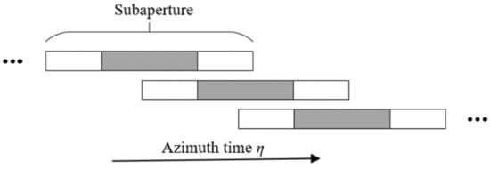
Figure 2.
Dividing overlapping subapertures.
Within any subaperture, the signal can be represented as , where and represent the start and end sampling time of the subaperture. The phase part in is
The quadratic phase not relevant to the slant error should be removed. Otherwise, it will affect estimating the double phase error gradient. So, we dechirp the as follows
where is the azimuth sampling time corresponding to the center of this subaperture. The phase part of is
As shown in Equation (13), the high-order phases in are all phase errors, so we can use them to estimate the double phase error gradients.
The estimation kernel is
where denotes conjugate. represents the phase gradient of one target in the subaperture, and is the step length of the estimation kernel. is the signal transformed from by performing center shifting and windowing [15].
2.2. Motion Error Estimation Model
The slant range error is expressed as
Its first-order Taylor expansion is as follows
If SAR is left side-looking, the slant range error is
where is the incident angle of the range bin of the target, such as . Although we consider the azimuth-variant slant range errors [16], at any azimuth time, for any target observed in the subaperture, the incident angle used in the Equation (17) is the azimuth-invariant angle , rather than the azimuth-variant actual incident angle .
The relationship between phase error and motion error is
After taking the second derivative, the relationship between the double-phase error gradient and the double-motion error gradient is
If SAR is right side-looking, the formulas are slightly different from the above, those are
When we obtain the estimated phase error (double gradient) (), we can use the linear relationship above to solve the motion errors (double gradients) and ( and ).
2.3. The Main Steps of WTA
The WTA is a robust method for trajectory estimation and autofocus [6]. The method is considered good in high-resolution conditions based on strong targets, which has been demonstrated by algorithm comparations in a recent study [7]. Since the signal models have been described in detail in Section 2.1 and Section 2.2, we briefly summarize the main steps of the WTA as follows.
- Estimating the double phase error gradients by PGA-based autofocus method: In the azimuth subapertures, dozens of strong targets are chosen to calculate the double phase error gradients based on the signals after the azimuth dechirp. The target-selection criteria [17] are used, which consider both the Doppler flatness and the energy.
- Filtering the double phase error gradients by polynomial fitting: By double integrating the estimated double phase error gradients and performing the polynomial fitting, the filtered phases are obtained. Then, the filtered double-phase gradients can be obtained by taking the second derivative of the above-fitted phases.
- Using the WTLS to solve the motion error estimation model: Compared to LS [18], Weighted Least Squares (WLS) [19], and TLS [20], the WTLS can obtain more accurate trajectory errors by utilizing the filtered double phase error gradients.
The step length of the estimation kernel (Equation (14)) in WTA is not considered, but is directly set to one. However, when the PRF is relatively high, this unconsidered way of setting is not reasonable. So, we improve the WTA by selecting the appropriate step, which is described in Section 4.
3. Accuracy Limits Analysis of Motion Error Estimation
3.1. Derivation of the CRLB
In the left side-looking, the CRLB of the motion error estimation is derived from Equation (18). At any azimuth time in a subaperture, suppose that strong targets are observed, and the estimated phase errors corresponding to these targets are
Use the phase error to solve the motion error :
Suppose , is independent Gaussian white noise, and the covariance matrix is .
In addition, suppose the coefficient matrices are
Equation (23) can be expressed as
The Fisher information matrix is square, and each element in the matrix is [21]
where
Substituting Formulas (28)–(31) into (27) yields the Fisher information matrix
The CRLB matrix can be obtained from the Fisher information matrix
According to Formula (33), the CRLB of motion error estimation in the x direction is
Similarly, the CRLB of motion error estimation in the z direction is
In the CRLB formulas, the numerator is the sum of terms, and the denominator is the sum of terms. The factors affecting the CRLB include target number , incident angle , wavelength , and variance of phase estimation error .
Similarly, the CRLB of the double motion error gradient estimation has the same form as above, except that represents the variance of the double phase error gradient estimation. In addition, the CRLB on the right side-looking is identical to the left side-looking.
3.2. Correctness Verification of the Derived CRLB
The WLS method is a valid estimation for the established model (Equation (23)) [22], which can reach the CRLB. Therefore, we can obtain the variance of WLS estimations through multiple random experiments and compare the variance with the CRLB, so as to verify the correctness of the CRLB formula.
The schematic diagram of the verification experiment is shown in Figure 3a. The parameters are set as follows. Supposing the wavelength is 0.0197m, the real motion error in the x direction is 0.1247 m, and in the z direction is 0.1430 m. For each observed target, the incident angle and the real phase error are set as shown in Table 1.

Figure 3.
(a) Schematic diagram of verification experiment; (b) The verification results of the CRLB.

Table 1.
Incident angles and real phase errors of verification experiment.
As for the phase estimation errors , we set six different groups of values as shown in Table 2. For example, in Group 1, the standard deviations of each target are °, °…°, and °, respectively, the average standard deviation of which is °. The average standard deviations of all groups are °, °…°, and °, respectively.
Table 2.
Phase estimation errors of verification experiment.
We add the phase estimation errors to the real phase errors to simulate the estimated phase errors , then use to solve motion errors and by WLS.
In each group, we conduct 20,000 random experiments to estimate and , then calculate the standard deviation of the estimation errors. At the same time, according to Equations (34) and (35), we use the parameters to calculate the square root of the CRLB.
As shown in Figure 3b, in each group (corresponding to each horizontal coordinate), the standard deviation of the estimation errors reaches the square root of the CRLB, which verifies the correctness of Equations (34) and (35).
3.3. Analysis of Influencing Factors of CRLB
We give the following conclusions about how the variables in the formula affect the CRLB.
- The shorter the wavelength, the smaller the CRLB.
- The smaller the variance , the smaller the CRLB.
- The more targets, the smaller the CRLB. When adding one target, the numerator of the formula increases by one term, while the denominator increases by terms. Because the denominator increases more than the numerator, the CRLB becomes smaller.
- The more extensive the incident angle range, the smaller the CRLB. When the range of incident angles increases, the difference between the incident angles increases. So, in the denominator increases and CRLB becomes smaller.
- When the incident angles increase, the CRLB in the x direction decreases and increases in the z direction. When the angles become larger, the numerator in the x direction is , which becomes smaller. The numerator in the z direction is , which becomes larger.
To verify conclusion 3, we conduct the following experiments. Randomly set the incident angles of the targets within the range of 20~60 degrees. The standard deviation of phase errors is designated as a uniform random number within 0~0.5 rad. When the target number is 10, 11… and 40, we calculate the CRLB, respectively. As shown in Figure 4a, the more targets, the smaller the CRLB.
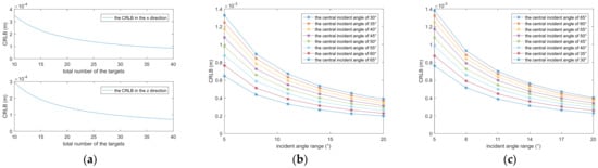
Figure 4.
(a) The variation in the CRLB with the targets’ number; (b) The variation in the CRLB with the incident angle in the x direction; (c) The variation in the CRLB with the incident angle in the z direction.
To verify conclusions 4 and 5, we calculate CRLB within the different angle ranges at different central incident angles. For example, set the central incident angle as 30 degrees, and put nine targets randomly within the incident angle range of . In addition, the central incident angle can also be changed, and we can set it as , respectively. As shown in Figure 4b,c, the variation in CRLB proves conclusions 4 and 5.
4. An Improved Track Error Estimation Method
4.1. Criteria of Step Length Selection
Selecting the appropriate step length should obey the following two criteria.
- The estimated double phase gradients should not be so large that Equation (36) exceeds the principal value interval. Otherwise, it will lead to phase wrapping [23].
- Track variation information cannot be lost. Increasing the step length is equivalent to down-sampling the track. We can use the a priori upper limit frequency information of the actual track to ensure that the track loss is within an acceptable range.
Here are the explanations for the second point. The typical motion errors of a high-precision UAV track in the actual flight are shown in Figure 5.

Figure 5.
(a) Typical motion error in the x direction; (b) Typical motion error in the z direction.
Fourier transform is performed on the above motion errors, and we can obtain the spectrum as shown in Figure 6. We can see the highest frequency is about , so the minimum sampling frequency should be , which provides a priori frequency limitation for selecting step length.

Figure 6.
(a) Spectrum of motion error in x direction; (b) Spectrum of motion error in z direction.
4.2. Method of Selecting Step Length
- When the step length defaults to one, like the WTA, we can obtain the estimated double-phase gradients. We use them to approximately calculate the standard deviation of phase estimation errors [6]. Then, we use the standard deviation and the other known parameters to calculate the CRLB. We can take the square root of CRLB to obtain . measures the estimation errors of the double-motion gradients. When is larger than the ground truth of the double motion gradients, the estimation errors lead to a pretty negative impact, which means we must select the appropriate step.
- To select the suitable step, we use the a priori weak navigation information and the basic parameters of scenes to conduct random experiments to estimate motion errors. From the experiments, we can obtain the root mean square error (RMSE) curve of estimation errors. The step length that minimizes the RMSE should be chosen as the appropriate one.
4.3. Overall Process of the Improved Method
The overall process of the proposed track error estimation method is as shown in Figure 7, which differs from the WTA in the addition of a selection of the estimation kernel step.
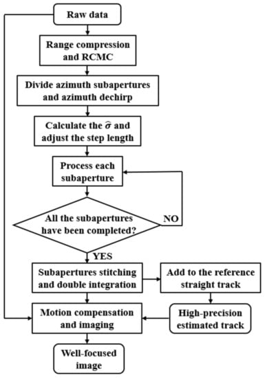
Figure 7.
The overall process of track error estimation.
5. Experiments and Results
5.1. Simulation Experiment Where PRF Is High
In Section 5.1, we conduct the simulation experiment where PRF is high. The parameters are in Table 3.
Table 3.
Parameters of simulation experiments.
Figure 8.
(a) The actual and reference track; (b) The target distribution diagram.
The incident angles of targets are shown in Table 4.
Table 4.
The incident angles of simulation experiments.
When we use the WTA, that is, the step length defaults to one, the simulation results at the SNR of 10 dB are as follows. In Figure 9a, the estimated double-phase gradients of a target are completely drowned by noise. In Figure 9b, due to the noise accumulation, the integral phase has an inflection point and deviates entirely from the ground truth. In Figure 9c, the final motion error estimation results are totally wrong, and are influenced by the above integral phase.

Figure 9.
(a) Double phase gradient estimation result; (b) Phase comparison after double integration; (c) Motion error estimation results when the step length defaults to 1 (simulation experiments).
Based on the accuracy analysis model, the calculated in the x and z directions are and , respectively. However, the real double-motion error gradients are both . It is obvious that the is much larger than the ground truth, so we should find the best step length.
We conduct the following random experiments. The step lengths range from 1 to 50. The RMSEs calculated by the estimated motion errors are shown in Figure 10. When the step length is 24 and the sampling frequency is 208 Hz, the RMSE reaches a minimum. Therefore, the suitable step length is 24.
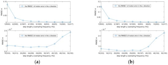
Figure 10.
(a) Variation in the RMSEs with different step lengths in the x direction (simulation experiments); (b) Variation in the RMSEs with different step lengths in the z direction (simulation experiments).
We estimate the track errors when the step is 24. The results are in Figure 11a, which performs much better than when the default step is selected. To compare the results of WTA and the proposed method, we put Figure 9c and Figure 11a together in Figure 11b, which illustrates the effectiveness of selecting the appropriate step length.
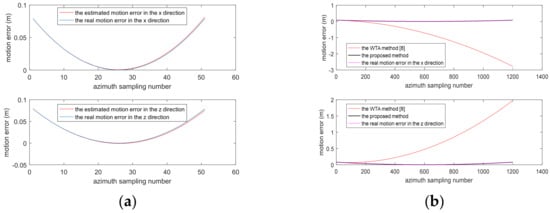
Figure 11.
(a) Motion error estimation results when (simulation experiments); (b) The comparative results of WTA and the proposed method.
5.2. Airborne SAR Data Experiment Where PRF Is Low
In Section 5.2, we perform airborne SAR data experiments. The parameters are in Table 5, where the PRF is relatively low.
Table 5.
Parameters of airborne SAR data.
When the step length defaults to one, the calculated is about 3 × 10⁻⁴ m. According to the a priori information, the ground truth of the double motion gradients is about 1 × 10⁻⁵ m.
The is slightly larger than the ground truth, so we perform experiments to select step length. The obtained RMSE curves of motion error estimation results are as shown in Figure 12.
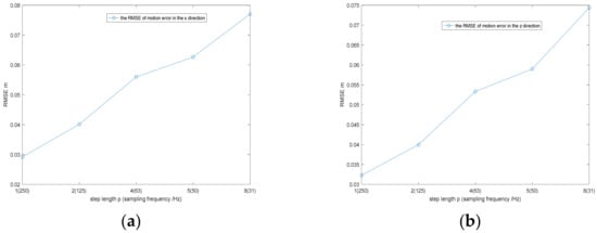
Figure 12.
(a) Variation in the RMSEs with different step lengths in the x direction (airborne SAR data experiments); (b) Variation in the RMSEs with different step lengths in the z direction (airborne SAR data experiments).
From the RMSE curve, we can decide that the step length of one is appropriate for the airborne SAR data. The reason for this phenomenon is that the PRF in this situation is relatively small.
After selecting the appropriate step, we estimate the track error on airborne SAR data. The motion error estimation results are shown in Figure 13a. As shown in Figure 13b, the estimation error in the x direction is within 2 cm and is within 3 cm in the z direction, realizing a high-precision estimation. To demonstrate the effectiveness of step length selection, we perform comparison experiments with the inappropriate step lengths of two and four. As shown in Figure 13c, the trajectory estimation accuracy becomes worse, and the estimation results exceed 0.05 m.
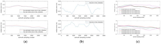
Figure 13.
(a) Motion error estimation results when p = 1 (airborne SAR data experiments); (b) Error estimation of motion errors when p = 1 (airborne SAR data experiments); (c) Comparison results of motion error estimation when p = 1, 2, 4 (airborne SAR data experiments).
Finally, we can use the estimated tracks for motion compensation [24,25] and imaging. Figure 14a presents the image without using the estimated track for motion compensation. Figure 14b–d present the images with motion compensation when the step length is 1, 2, and 4, respectively. Figure 14e–h show the calibration reflector’s imaging quality after upsampling 16 times. From Figure 14, when we choose the appropriate step to estimate track error, and use the estimated track to perform motion compensation and imaging, we can obtain well-focused images.


Figure 14.
(a) Defocused image without using the estimated track for motion compensation; (b) Well-focused image with motion compensation when p = 1; (c) Focused image with motion compensation when p = 2; (d) Focused image with motion compensation when p = 4; (e) Calibration reflector of the defocused image after upsampling 16 times; (f) Calibration reflector of the well-focused image after upsampling 16 times when p = 1; (g) Calibration reflector of the focused image after upsampling 16 times when p = 2; (h) Calibration reflector of the focused image after upsampling 16 times when p = 4.
We also compare the calibration reflector’ focusing quality in the azimuth direction. As shown in Figure 15a, the quality when performing the motion compensation is better than that without motion compensation. As shown in Figure 15b, the quality when the step is appropriate is the best.

Figure 15.
(a) Focusing quality comparison between performing motion compensation (p = 1) and not performing motion compensation in the azimuth direction; (b) Focusing quality comparison when p = 1, 2, 4 in the azimuth direction.
6. Discussions
If the azimuth resolution is higher or if the flight velocity is faster, for example, where the velocities of some manned aircraft reach several hundred meters per second, then the PRF of the airborne SAR system will be higher. At this time, we note that the step cannot be directly set to one like the WTA, so we propose the solution of selecting the best step to improve the applicability of WTA to various PRFs.
Moreover, in the method of this paper and in many current studies, the trajectory estimation is performed on the raw data. So, in the future, we can try to make more use of the weak navigation information, which may improve the estimation accuracy or enable the method to be used in ultra-high-resolution conditions.
7. Conclusions
In this paper, we derive for the first time the CRLB of the motion error estimation model widely used in many studies, and propose a more robust improvement of the WTA. The proposed step selection method can solve the limitation of WTA to use the default step, enabling WTA to obtain precise track estimation results under different parameters.
Author Contributions
Conceptualization, M.G. and X.Q.; Funding acquisition, X.Q. and C.D.; Investigation, M.G.; Methodology, M.G. and X.Q.; Resources, X.Q. and Y.C.; Writing—original draft, M.G.; Writing—review and editing, M.G., X.Q. and J.L. All authors have read and agreed to the published version of the manuscript.
Funding
This research was funded by the National Key R&D Program of China under Grant No.2018YFA0701903, and also by the NSFC No. 62022082.
Conflicts of Interest
The authors declare no conflict of interest.
References
- Wiley, C.A. Synthetic Aperture Radars. IEEE Trans. Aerosp. Electron. Syst. 1985, AES-21, 440–443. [Google Scholar] [CrossRef]
- Xing, M.; Jiang, X.; Wu, R.; Zhou, F.; Bao, Z. Motion compensation for UAV SAR based on raw radar data. IEEE Trans. Geosci. Remote Sens. 2009, 47, 2870–2883. [Google Scholar] [CrossRef]
- Bejiga, M.B.; Zeggada, A.; Nouffidj, A.; Melgani, F. A convolutional neural network approach for assisting avalanche search and rescue operations with UAV imagery. Remote Sens. 2017, 9, 100. [Google Scholar] [CrossRef]
- Liang, Y.; Li, G.; Wen, J.; Zhang, G.; Dang, Y.; Xing, M. A fast time-domain SAR imaging and corresponding autofocus method based on hybrid coordinate system. IEEE Trans. Geosci. Remote Sens. 2019, 57, 8627–8640. [Google Scholar] [CrossRef]
- Bezvesilniy, O.O.; Gorovyi, I.M.; Vavriv, D.M. Autofocusing SAR images via local estimates of flight trajectory. Int. J. Microw. Wirel. Technol. 2016, 8, 881–889. [Google Scholar] [CrossRef]
- Li, Y.; Liu, C.; Wang, Y.; Wang, Q. A robust motion error estimation method based on raw data. IEEE Trans. Geosci. Remote Sens. 2012, 50, 2780–2790. [Google Scholar] [CrossRef]
- Li, J.; Chen, J.; Wang, P.; Loffeld, O. A Coarse-to-Fine Autofocus Approach for Very High-Resolution Airborne Stripmap SAR Imagery. IEEE Trans. Geosci. Remote Sens. 2018, 56, 3814–3829. [Google Scholar] [CrossRef]
- Ran, L.; Liu, Z.; Zhang, L.; Li, T.; Xie, R. An autofocus algorithm for estimating residual trajectory deviations in synthetic aperture radar. IEEE Trans. Geosci. Remote Sens. 2017, 55, 3408–3425. [Google Scholar] [CrossRef]
- Sjanic, Z.; Gustafsson, F. Simultaneous navigation and SAR auto-focusing. In Proceedings of the 2010 13th International Conference on Information Fusion, Edinburgh, UK, 26–29 July 2010; pp. 1–7. [Google Scholar]
- Pu, W.; Wu, J.; Huang, Y.; Yang, J.; Yang, H. Fast factorized backprojection imaging algorithm integrated with motion trajectory estimation for bistatic forward-looking SAR. IEEE J. Sel. Top. Appl. Earth Obs. Remote Sens. 2019, 12, 3949–3965. [Google Scholar] [CrossRef]
- Hu, K.; Zhang, X.; He, S.; Zhao, H.; Shi, J. A less-memory and high-efficiency autofocus back projection algorithm for SAR imaging. IEEE Geosci. Remote Sens. Lett. 2014, 12, 890–894. [Google Scholar]
- Torgrimsson, J.; Dammert, P.; Hellsten, H.; Ulander, L.M.H. An efficient solution to the factorized geometrical autofocus problem. IEEE Trans. Geosci. Remote Sens. 2016, 54, 4732–4748. [Google Scholar] [CrossRef]
- Chen, J.; Xing, M.; Yu, H.; Liang, B.; Peng, J.; Sun, G.C. Motion Compensation/Autofocus in Airborne Synthetic Aperture Radar: A Review. IEEE Geosci. Remote Sens. Mag. 2022, 10, 185–206. [Google Scholar] [CrossRef]
- Chen, Z.; Zhang, Z.; Zhou, Y.; Wang, P.; Qiu, J. A novel motion compensation scheme for airborne very high resolution SAR. Remote Sens. 2021, 13, 2729. [Google Scholar] [CrossRef]
- Wahl, D.E.; Eichel, P.H.; Ghiglia, D.C.; Jakowatz, C.V. Phase gradient autofocus-a robust tool for high resolution SAR phase correction. IEEE Trans. Aerosp. Electron. Syst. 1994, 30, 827–835. [Google Scholar] [CrossRef]
- Prats, P.; Camara, D.; Reigber, A.; Scheiber, R.; Mallorqui, J.J. Comparison of Topography- and Aperture-Dependent Motion Compensation Algorithms for Airborne SAR. IEEE Geosci. Remote Sens. Lett. 2007, 4, 349–353. [Google Scholar] [CrossRef]
- Chan, H.L.; Yeo, T.S. Noniterative quality phase-gradient autofocus (QPGA) algorithm for spotlight SAR imagery. IEEE Trans. Geosci. Remote Sens. 1998, 36, 1531–1539. [Google Scholar] [CrossRef]
- Chen, J.; Liang, B.; Zhang, J.; Yang, D.G.; Deng, Y.; Xing, M. Efficiency and Robustness Improvement of Airborne SAR Motion Compensation With High Resolution and Wide Swath. IEEE Geosci. Remote Sens. Lett. 2022, 19, 1–5. [Google Scholar] [CrossRef]
- Zhang, L.; Qiao, Z.; Xing, M.; Yang, L.; Bao, Z. A Robust Motion Compensation Approach for UAV SAR Imagery. IEEE Trans. Geosci. Remote Sens. 2012, 50, 3202–3218. [Google Scholar] [CrossRef]
- Scharf, L.L. Statistical Signal Processing: Detection, Estimation, and Time Series Analysis; Addison-Wesley Publishing Company: Boston, MA, USA, 1991. [Google Scholar]
- Stoica, P.; Moses, R.L. Spectral Analysis of Signals; Pearson Prentice Hall: Upper Saddle River, NJ, USA, 2005; Volume 452. [Google Scholar]
- Kay, S.M. Fundamentals of Statistical Signal Processing: Estimation Theory; Prentice-Hall, Inc.: Hoboken, NJ, USA, 1993. [Google Scholar]
- Pu, L.; Zhang, X.; Zhou, Z.; Li, L.; Zhou, L.; Shi, J.; Wei, S. A Robust InSAR Phase Unwrapping Method via Phase Gradient Estimation Network. Remote Sens. 2021, 13, 4564. [Google Scholar] [CrossRef]
- Chen, J.; Zhang, J.; Yu, H.; Xu, G.; Liang, B.; Yang, D.G.; Wang, H. Blind NCS-Based Autofocus for Airborne Wide-Beam SAR Imaging. IEEE Trans. Comput. Imaging 2022, 8, 626–638. [Google Scholar] [CrossRef]
- Macedo, K.A.C.d.; Scheiber, R. Precise topography- and aperture-dependent motion compensation for airborne SAR. IEEE Geosci. Remote Sens. Lett. 2005, 2, 172–176. [Google Scholar] [CrossRef]


Publisher’s Note: MDPI stays neutral with regard to jurisdictional claims in published maps and institutional affiliations. |
© 2022 by the authors. Licensee MDPI, Basel, Switzerland. This article is an open access article distributed under the terms and conditions of the Creative Commons Attribution (CC BY) license (https://creativecommons.org/licenses/by/4.0/).