Fusion and Analysis of Land Use/Cover Datasets Based on Bayesian-Fuzzy Probability Prediction: A Case Study of the Indochina Peninsula

Abstract

Land use/cover (LUC) datasets are the basis of global change studies and cross-scale land planning. Data fusion is an important direction for correcting errors and improving the reliability of multisource LUC datasets. In this study, a new fusion method based on Bayesian fuzzy probability prediction was developed, and a case study was conducted in five countries of the Indochina Peninsula to form a fusion dataset with a resolution of 30 m in 2020 (BeyFusLUC30). After precision and uncertainty analysis, it was found that: (1) using accuracy validation information as prior knowledge and considering spatial relations can be well applied to LUC data fusion. (2) When compared to the four source datasets (LSV10, GLC_FCS30, ESRI10, and Globeland30), the accuracy indices of BeyFusLUC30 are all optimal. The average overall consistency increased by 6.42–13.61%, the overall accuracy increased by 4.84–7.11%, and the kappa coefficient increased by 4.98–7.60%. (3) The accuracy of the fusion result improved less for land types with good original accuracy (cropland, forest, water area, and built-up land), and the improved range of F1 score was at least 0.40–2.29%, and at most 6.66–9.88%. For the land types with poor original accuracy (grassland, shrubland, wetland, and bare land), the accuracy of the fusion result improved more, and the F1 score improved by at least 4.02–5.82%, and at most 14.41–48.35%. The LUC dataset fusion and quality improvement method developed in this study can be applied to other regions of the world as well. BeyFusLUC30 can provide reliable LUC data for scientific research and government applications in the peninsula.

1. Introduction

Natural and anthropogenic causes influence land use/cover (LUC) [1]. It reflects the natural properties of land and the impact of human activities and is of great significance for economic and social development, ecological environment assessment, regional food security, and global and national development strategies [2,3]. LUC datasets can provide basic data support for a wide range of research fields [4,5].

Many global-scale mid- and high-resolution LUC products are freely available for download and use [6]. Some well-known products include European Space Agency’s CCI Land Cover series (https://www.esa-landcover-cci.org/, accessed on 2 April 2022) and GlobCover series (https://www.esa.int/, accessed on 5 April 2022) [7,8]; Copernicus Programme’s CGLS-LC100 series (https://land.copernicus.eu/, accessed on 5 April 2022) [9]; National Aeronautics and Space Administration’s MODIS Land Cover series (https://lpdaac.usgs.gov/, accessed on 5 April 2022) [10]. Their resolution is typically a few hundred meters to one kilometer. With the rapid expansion of remote sensing (RS) observation platforms, the enhancement of RS cloud computing capability, and the advancement of LUC mapping technology over the last decade, the spatial resolution of LUC datasets has been continuously improved [11]. The Globeland30 dataset (http://www.globallandcover.com/, accessed on 5 April 2022), developed by the Ministry of Natural Resources of China, contains global data with a 30 m resolution in 2000, 2010, and 2020 [12]. GLC_FCS30 dataset (https://data.casearth.cn/, accessed on 5 April 2022) developed by the Aerospace Information Research Institute, Chinese Academy of Sciences, which is updated every five years, contains global data with a 30 m resolution from 1985 to 2020 [13,14]. LSV10 dataset (https://esa-worldcover.org/, accessed on 5 April 2022), developed by the European Space Agency, contains global data with a 10 m resolution in 2020 [15]. The ESRI Land Cover dataset (ESRI10, https://www.arcgis.com/, accessed on 5 April 2022), developed by the Environmental Systems Research Institute and updated yearly, contains global data with a 10 m resolution in 2017–2021 [16].

These LUC datasets are convenient for researchers worldwide to conduct research in the fields of nature, resources, and ecology [17,18,19]. However, they may differ regarding the type, quantity, accuracy, and spatial consistency because of the different RS images, classification systems, and mapping methods employed [20]. A single LUC dataset might sometimes fail to fulfill the reliability criteria of research and applications [11]. In the context of multisource data coexistence and integration research, integrating information from existing data to form new LUC data products is a significant path to overcoming this challenge [21,22].

Many researchers have studied LUC data fusion, which has produced a batch of reliable and practical products on a regional or global scale [23,24]. See et al. [25] used a spatial consistency and geographically weighted regression method to determine the consistent location in the source datasets (GLC2000, GlobCover, and MODIS Land Cover) and then assigned the attribute with the highest consistency to the pixels. Select the surrounding LUC samples for the location with no consistency to carry out geographically weighted regression and assign the attribute with the highest probability of accuracy to the pixels. The generated medium-resolution LUC dataset has better accuracy than the source datasets. Fritz et al. [26] proposed a convergence of evidence approach to rank different products (GLC2000, MODISLC 2005, GlobCover 2005, GEOCOVER, Cropland probability layer) using crowdsourced data from Geo-Wiki. Statistical data is then used for calibration to finally allocate cropland within each country and sub-national unit, resulting in a fusion data product that is superior to the input data. Lu et al. [27] proposed a hierarchical optimization synergy approach to form the 2010 China cropland dataset by fusing five existing cropland products (GlobeLand30, CCI-LC, GlobCover 2009, MODIS C5, MODIS Cropland). The accuracy evaluation shows that the spatial location accuracy of the result is higher than the existing five datasets, and the consistency with the statistics is better. Bai et al. [28] combined expert scoring and semantic correlation to build an evidence fusion method and fused five global LUC datasets (GLCC, UMD, GLC2000, MODIS LC, and GlobCover) to form a global 1 km fusion LUC dataset (SYNLCover). SYNLCover includes 8 first-level and 12 fine types, and its consistency is significantly improved. Pérez-Hoyos et al. [29] used a multi-criteria analysis method that considered five factors, including timeliness, resolution, FAO statistical data, accuracy, and expert assessment, combined with manual fine-tuning. The source datasets (CGLS-LC, GLC2000, GLCNMO, GlobCover, GlobeLand30, CCI-LC, MODIS Land Cover) were fused to form African grassland and cropland datasets with 250 m resolution, providing reliable support for agricultural monitoring in Africa.

These fusion datasets provide high-quality alternatives for both scholars and managers. However, there are problems in existing research cases, such as large year disparities in source datasets, large spatial resolution differences, and uneven data quality, all of which are important factors that affect the reliability of the results. On the other hand, the existing fusion methods also have some problems, such as (1) pixel attributes are selected from the same location of the source datasets, which cannot effectively correct the common errors in the source datasets; (2) Only the land types possessed by all source datasets can be fused, and the fine types information possessed by only a few datasets cannot be fully utilized; (3) Expert scoring and multi-criteria analysis cannot avoid the influence of subjective factors; (4) Most methods cannot effectively consider the spatial relationships that play an important role in land classification. The Bayesian posterior probability principle is similar to LUC dataset error correction and multisource information fusion. Combining the Bayesian probability principle with the spatial neighborhood relation, a new LUC data set fusion method can overcome the above problems. This is a feasible approach worth exploring further.

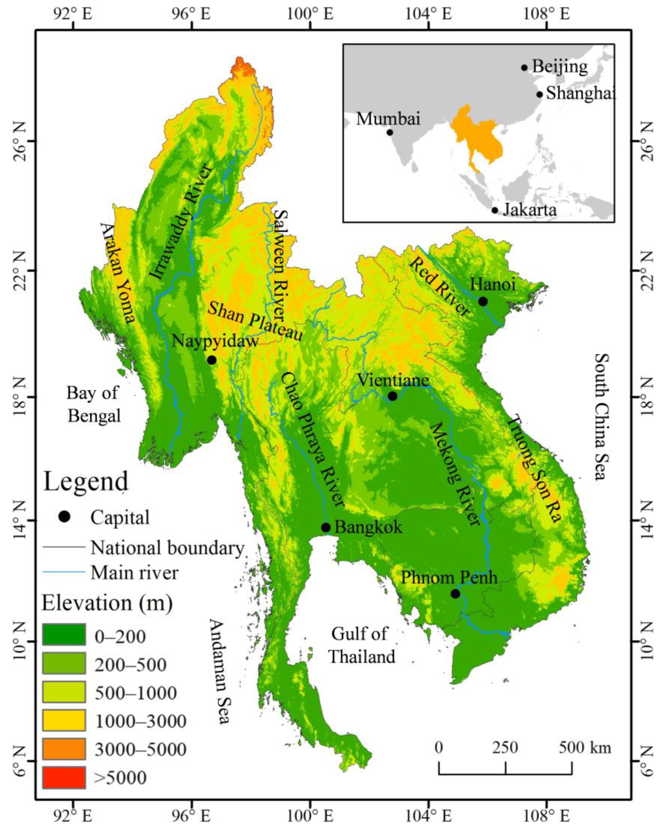
The Indochina Peninsula is a vital link between East and South Asia. It has an important geopolitical and geo-economics status. Furthermore, it is important in China’s “six corridors and six channels” infrastructure construction planning. The Indochina Peninsula is mostly underdeveloped and lacks regional- or national-scale LUC datasets. The development of fusion LUC products with good timeliness, high resolution, and high reliability in this area will be a vital approach for researchers and developers to understand and enter this area.

Therefore, we intend to develop a fusion method to eliminate the influence of subjective factors and introduce spatial relations and Bayesian probabilities. Four high-resolution LUC products (LSV10, GLC_FCS30, ESRI10, and Globeland30) were selected for fusion research and analysis in five Indochina Peninsula nations (Myanmar, Vietnam, Thailand, Cambodia, and Laos). This study aimed to achieve the following three objectives:

(1) Develop a LUC data-fusion method based on Bayesian fuzzy probability prediction;

(2) Generate a 30 m resolution fusion LUC product for the Indochina Peninsula in 2020 based on the LSV10, GLC_FCS30, ESRI10, and Globeland30 datasets;

(3) Evaluate the overall accuracy and type accuracy of the fusion dataset, provide a reference for researchers on the fusion method and provide a precision reference for selecting and using the fusion dataset.

2. Case Area and Data

2.1. Case Area

The Indochina Peninsula is located between China and South Asia. Its longitude and latitude range is roughly 92.0°E–109.5°E, 5.5°N–28.5°N. The case study area includes Vietnam, Laos, Cambodia, Myanmar, and Thailand, with a total area of 2.065 × 106 km² (Figure 1).

The Indochina Peninsula is in a tropical monsoon climate zone, with high temperatures throughout the year. Further, it can be divided into two seasons: dry and rainy. The terrain is high in the north and low in the south, with plateaus, hills, and mountains in the north and estuarine deltas and alluvial plains in the south [30]. The major mountains are Arakan Yoma in the west, a series of mountains extending southward from the Shan Plateau in the middle, and Truong Son Ra in the east. The main rivers are the Irrawaddy, Salween, Chao Phraya, Mekong, and Red Rivers.

In 2018, the total population of the five countries was 0.242 × 10⁹, accounting for 3.10% of the world’s total population, with a GDP of 0.864 × 10¹² US dollars, accounting for 1.01% of the global economic aggregate [6]. Compared with the population, the global share of regional economic aggregates lags significantly. The proportion of the added value of the primary, secondary, and tertiary industries is approximately 12%, 52%, and 36%, respectively, indicating that the region is in an early stage of industrialization [31].

2.2. LUC Datasets

There are significant differences in the status, resolution, and accuracy of the existing LUC datasets owing to various hyperspectral and/or multispectral aerial images, land classification systems, LUC mapping methods, and different release timings. This study selected four LUC datasets with the best current situation (2020), high resolution (10 m–30 m), and high overall accuracy (74–86%), namely: LSV10 [15], GLC_FCS30 [13,14], ESRI10 [16], and Globeland30 [12]. The information is presented in

Table 1. Information about the source datasets.

Dataset	Images	Time	Classification System	Number of Types	Resolution (m)	Overall Accuracy (%)
LSV10	Sentinel-1, Sentinel-2	January 2020–December 2020	LCCS	11	10	74.4
GLC_FCS30	Landsat, Sentinel	2019–2020	Self-defined	30	30	81.4
ESRI10	Sentinel-2	January 2020–December 2020	Self-defined	10	10	85.96
Globeland30	Landsat8, GF-1	Vegetation growth season within two years before and after 2020	Self-defined	10	30	85.72

.

2.3. Data Pre-Processing

Preprocessing was performed on the source datasets, including stitching and cropping, projection transformation, and upscaling.

First, we stitched the downloaded data and converted them to the same coordinate system (WGS_1984_UTM_Zone_47N) and then used the case study area boundary to crop them. Finally, we used the pixel aggregation method to upscale LSV10 and ESRI10 to a resolution of 30 m, consistent with GLC_FCS30 and Globeland30.

3. Method

3.1. Overall Technical Route

The realization process of this research can be divided into six steps, as shown in Figure 2. They are as follows: (1) Build the target LUC classification system and merge the source LUC datasets on a unified basis. (2) The accuracy verification information of the source LUC datasets is used to evaluate the overall misclassification among land types to determine the prior probability. (3) Based on the Bayesian posterior probability formula and the introduction of spatial neighborhood relation, improve the posterior probability calculation method. A posteriori probability is calculated based on the improved method. (4) Considering the accuracy and reliability of the LUC datasets, the weighted average method is used to synthesize the posterior probability results of the source LUC datasets. By assigning the attribute with the highest synthetic posterior probability to the pixel, the fuzzy probability fusion is realized, and the first-level types fusion result is obtained. (5) According to the detailed classification information of GLC_FCS30, the second-level classification of cropland and forest was carried out according to the spatial correlation principle and neighborhood search method. (6) From the two aspects of consistency and validation accuracy of the datasets, the accuracy of fusion results was tested by using six indexes, namely average overall consistency, overall accuracy (OA), Kappa coefficient, user accuracy (UA), producer accuracy (PA) and F1 score.

3.2. Merge LUC Types

Since the source LUC datasets use different land classification systems, they must be merged into a unified system. Drawing on previous research experience [32,33], we initially identified nine common first-level types: cropland, forest, grassland, shrubland, wetland, water bodies, built-up land, bare land, and snow and ice, which were coded in multiples of 10 from 10 to 90. Considering the important roles of croplands and forests (diverse ecosystems and important economic sectors), we further subdivided cropland into two second-level types: rainfed cropland and irrigated cropland, coded as 11 and 12, respectively, and subdivided forests into six second-level types: evergreen broadleaved forest, deciduous broadleaved forest, evergreen needle-leaved forest, deciduous needle-leaved forest, mixed leaf forest, and fruit forest (orchard), coded in order from 21 to 26, respectively. Therefore, the land classification system constructed in this study includes 15 types that are both refined and practical.

We then merge the source datasets into the constructed classification system. It can be noted that only GLC_FCS30 has fine second-level type information, and the other three have only first-level type information. The merging process strictly follows the definition and description of the source data type. We have also made the necessary adjustments. For example, GLC_FCS30 classifies the Orchard as a second-level type of cropland, and we merge it into a second-level type of forest. This is more in line with the ecosystem [6]. For overly detailed types in GLC_FCS30, we merge them into the same type. For example, we combine the Shrubland (120), Evergreen shrubland (121), and Deciduous shrubland (122) in GLC_FCS30 into the Shrubland (40) in the constructed system. The LUC codes and meanings of the source and merged datasets are presented in detail in

Table 2. LUC codes and meanings of the source datasets and merged codes.

LSV10			GLC_FCS30									ESRI10			Globeland30
Code	Meaning	Merged Code	Code	Meaning	Merged Code	Code	Meaning	Merged Code	Code	Meaning	Merged Code	Code	Meaning	Merged Code	Code	Meaning	Merged Code
10	Tree cover	20	10	Rainfed cropland	11	82	Closed deciduous needle-leaved forest (fc > 0.4)	24, /	180	Wetlands	50	1	Water	60	10	Cultivated land	10
20	Shrubland	40	11	Herbaceous cover	11	91	Open mixed leaf forest (broadleaved and needle-leaved)	25, /	190	Impervious surfaces	70	2	Trees	20	20	Forest	20
30	Grassland	30	12	Tree or shrub cover (Orchard)	26	92	Closed mixed leaf forest (broadleaved and needle-leaved)	25, /	200	Bare areas	80	3	Grass	30	30	Grassland	30
40	Cropland	10	20	Irrigated cropland	12	120	Shrubland	40	201	Consolidated bare areas	80	4	Flooded vegetation	50	40	Shrubland	40
50	Built-up	70	51	Open evergreen broadleaved forest	21	121	Evergreen shrubland	40	202	Unconsolidated bare areas	80	5	Crops	10	50	Wetland	50
60	Bare/sparse vegetation	80	52	Closed evergreen broadleaved forest	21	122	Deciduous shrubland	40	210	Waterbody	60	6	Scrub/shrub	40	60	Water bodies	60
70	Snow and Ice	90	61	Open deciduous broadleaved forest (0.15 < fc < 0.4)	22	130	Grassland	30	220	Permanent ice and snow	90	7	Built Area	70	70	Tundra	80, /
80	Permanent water bodies	60	62	Closed deciduous broadleaved forest (fc > 0.4)	22	140	Lichens and mosses	80, /	250	Filled value	/	8	Bare ground	80	80	Artificial surfaces	70
90	Herbaceous wetland	50	71	Open evergreen needle-leaved forest (0.15 < fc < 0.4)	23	150	Sparse vegetation (fc < 0.15)	80				9	Snow/Ice	90	90	Bare land	80
95	Mangroves	50	72	Closed evergreen needle-leaved forest (fc > 0.4)	23	152	Sparse shrubland (fc < 0.15)	80				10	Clouds	/	100	Permanent snow and ice	90
100	Moss and lichen	80, /	81	Open deciduous needle-leaved forest (0.15 < fc < 0.4)	24, /	153	Sparse herbaceous (fc < 0.15)	80

Note: fc = forest cover; / indicates that this land type was not included in the case study area data.

.

3.3. Definition of Prior Probability

The degree of misclassification between land types in the LUC datasets indicates the degree of confusion. From the perspective of probability theory, when the total amount is sufficiently large, the frequency of an event reflects its probability [34]. The misclassification frequency can be used to characterize the misclassification probability. The formulae are as follows:

$$R\left(A_i|A_j\right)=\frac{S(A_i|A_j)}{S\left(A_j\right)}$$

(1)

$$P\left(A_i|A_j\right)=R\left(A_i|A_j\right)$$

(2)

where $A_i$ and $A_j$ are the the ith and jth types of land use/cover in the LUC dataset, respectively; $R\left(A_i|A_j\right)$ is the ratio of classifying $A_j$ as $A_i$; $S(A_i|A_j)$ is the area of classifying $A_j$ as $A_i$, in km²; $S\left(A_j\right)$ is the area of $A_j$, in km²; $P(A_i|A_j)$ is the probability of classifying $A_j$ as $A_i$.

In developing the source LUC datasets, the original authors performed accuracy validation and released the results based on global stratified sampling and cross-validation. Their error matrices reflect the overall misclassification. This information can be used to calculate prior probabilities.

3.4. Posterior Probability Calculation Introducing Spatial Relationships

According to the Bayesian posterior probability formula [35,36], if a pixel has been classified as a land type by the LUC dataset, the probability that the pixel belongs to another (or the same) type can be calculated using the following formula:

$$P\prime \left(A_j|A_i\right)=\frac{P(A_i|A_j)\times P\left(A_j\right)}{P\left(A_i\right)}$$

(3)

$$P\left(A_i\right)={\displaystyle \sum }_{j=1}^{M}P\left(A_i|A_j\right)\times P\left(A_j\right)=R\left(A_i\right)$$

(4)

where $A_i$ and $A_j$ are the ith and jth types of land use/cover in the LUC dataset, respectively; $P\prime \left(A_j|A_i\right)$ is the probability that the pixel is actually $A_j$ when the LUC dataset has classified it as $A_i$, that is, the posterior probability; $P\left(A_i\right)$ is the probability that $A_i$ is in the dataset, and the value is equal to the area ratio of $A_i$ ($R\left(A_i\right)$).

There is a strong geographical correlation in the spatial distribution of land use/cover, and the same type of land often shows obvious spatial aggregation characteristics [37,38]. Therefore, continuity and spatial distribution are important for developing LUC datasets. Similarly, considering the spatial relationship in the fusion of LUC datasets is an important direction for improving the accuracy of the results. To this end, this study introduces a neighborhood window and improves the posterior probability calculation formula.

The specific method is to construct a neighborhood window of an appropriate size with the target pixel as the center, count the frequencies of various types of land in the window, and use the window frequency to substitute its frequency in the dataset in the posterior probability calculation. The improved formula is as follows:

$$P\prime \left(A_j|A_i\right)=\frac{P(A_i|A_j)\times R_w\left(A_j\right)}{R_w\left(A_i\right)}$$

(5)

where $P\prime \left(A_j|A_i\right)$ is the probability that the target pixel is actually $A_j$ when the LUC dataset has classified it as $A_i$; $w$ is the neighborhood window, which is a square of 9 × 9 pixels in this study; $R_w\left(A_i\right)$ and $R_w\left(A_i\right)$are the proportions of $A_i$ and $A_j$ in $w$, respectively.

3.5. Fusion Based on Fuzzy Probability

According to formula 5, the posterior probabilities of the nine first-level types of the four LUC datasets can be obtained pixel-by-pixel. Taking a pixel of LSV10 as an example, we now have the probability that it belongs to cropland, to forest, to grassland… (9 first-level types). The same is true for GLC_FCS30, ESRI10, and Globeland30.

After that, we need to synthesize the posterior probabilities of four LUC datasets into an indicator to obtain the synthetic probability so that it is convenient to assign a land type to the pixel (fusion result). Taking cropland as an example, each of the four LUC datasets has a value at the location of a pixel, indicating the probability that the pixel belongs to cropland. Through the process of probability synthesis, the four values become one value, which indicates the probability that the pixel belongs to the cropland. The same applies to forest, grassland, etc. (the other 8 first-level types).

Considering the differences in accuracy and credibility of different LUC datasets, this study used the weighted average method to synthesize the posterior probability results of the four datasets to form a comprehensive posterior probability (CPP). The formula used is as follows:

$$P_c\prime \left(A_j\right)=\frac{{{\displaystyle \sum }}_{L=1}^N{P}_{L,c}\left(A_j\right)\times O{A}_L}{N}$$

(6)

where $A_j$ is the jth type of land use/cover; $P_c\prime \left(A_j\right)$is the CPP of $A_j$ on pixel c; $N$ is the number of LUC datasets, which is 4 in this paper; $P_{L,c}\left(A_j\right)$ is the posterior probability of $A_j$ on pixel c in the Lth LUC dataset; $O{A}_L$ is the overall accuracy of the Lth LUC dataset.

Then, for each pixel, we compared the CPP of nine first-level types and assigned the land type with the largest CPP to the pixel. Take a pixel, for example. We have now acquired the probability that it belongs to cropland, forest, grassland, etc. (9 first-level types). We select the largest value and assign the corresponding land type to the pixel.

The formula used is as follows:

$$A_c=\left\{A_n\right| P_c\prime \left(A_n\right)=MAX\left(P_c\prime \left(A_i\right)\right), i=1, 2, \cdots , M\}$$

(7)

where $A_c$ is the finalized land use/cover type on pixel c; $P_c\prime \left(A_i\right)$is the CPP of $A_i$ on pixel c; $M$ is the number of first-level types, which is nine in this study, $MAX$ is a function used to find the maximum value.

3.6. Second-Level Classification

Like the first-level types, the second-level types of cropland and forest have spatial continuity and repetition. The same second-level type tends to cluster spatially and geographically, and two parcels of land adjacent to each other are likely to share the same properties [18]. Therefore, based on obtaining the first-level type fusion result, this study refers to the detailed classification information of the GLC_FCS30 dataset and conducts the second-level classification of cropland and forest according to the principle of spatial correlation.

First, it needs to be clear that there are two situations: the fusion result is the same as GLC_FCS30, or the fusion result is different from GLC_FCS30. This is the basis for our next steps.

Taking cropland as an example, for each cropland pixel in the fusion result, there are two situations. GLC_FCS30 identifies the pixel as cropland; GLC_FCS30 identifies the pixel as other land types. For the former case, we directly assign the second-level attribute of GLC_FCS30 to this pixel. For the latter case, we use the neighborhood search method to assign the second-level attribute of the nearest GLC_FCS30 cropland pixel to this pixel. So far, we have completed the second-level classification of all cropland pixels in the first-level fusion results.

For forest pixels, the second-level classification strategy was the same as for cropland.

3.7. Accuracy Validation

This study compares and analyzes the overall consistency, overall accuracy, Kappa coefficient, user accuracy, producer accuracy, F1 score of the fusion result, and the source LUC datasets of the first-level type from the aspects of dataset consistency and validation accuracy.

The consistency check can analyze all the pixels in the LUC datasets, revealing their consistent level of quantification. In the specific implementation process, first, the five datasets (fusion result and source datasets) were paired to calculate the overall consistency (OC) of each combination. The overall consistency of the four combinations in which each dataset is located is then arithmetically averaged to obtain the average overall consistency (AOC). The formula used is as follows:

$$OC\left(i,j\right)=\frac{CA\left(i,j\right)}{S}$$

(8)

$$AOC\left(i\right)=\frac{{{\displaystyle \sum }}_{j=1}^{N}OC\left(i,j\right)}{N},i\ne j$$

(9)

where $i$ and $j$ are the ith and jth LUC datasets, respectively;$OC\left(i,j\right)$ is the overall consistency of the$i$/$j$ combination; $CA\left(i,j\right)$ is the consistent area in the $i$/$j$ combination, in km²; $S$ is the total area of the region, in km²; $AOC\left(i\right)$ is the average overall consistency between $i$ and the other datasets; $N$ is the number of combinations containing $i$, which is four in this study.

The F1 score is an indicator used in statistics to measure the accuracy of dichotomous models. The core idea is that a high score requires not only high precision (producer accuracy) and recall (user accuracy) but also a small difference between the two [39]. The formulae are as follows:

$$P\left(A_i\right)=\frac{N\left(A_i,A_i\right)}{{{\displaystyle \sum }}_{j=1}^{M}N\left(A_j,A_i\right)}$$

(10)

$$R\left(A_i\right)=\frac{N\left(A_i,A_i\right)}{{{\displaystyle \sum }}_{j=1}^{M}N\left(A_i,A_j\right)}$$

(11)

$$F1\left(A_i\right)=\frac{2\times P\left(A_i\right)\times R\left(A_i\right)}{P\left(A_i\right)+R\left(A_i\right)}$$

(12)

where $A_i$ and $A_j$ are the the ith and jth types of land use/cover, respectively; $P\left(A_i\right)$, $R\left(A_i\right)$, and $F1\left(A_i\right)$ are the precision, recall, and F1 score of $A_i$, respectively; $N\left(A_i,A_i\right)$ is the number of pixels that misclassify $A_j$ as $A_i$; $N\left(A_i,A_i\right)$ is the number of pixels that are correctly classified as $A_i$; $M$ is the number of land types, which is nine in this study.

The overall accuracy is a commonly used indicator for validating classification results. It is the ratio of correctly classified pixels to all pixels and reflects the overall credibility [40]. The Kappa coefficient is also an overall accuracy evaluation index; however, it not only considers the overall accuracy but also the balance of the accuracy of each type, increasing the influence of the type with a small area in the results [41]. The formulae are as follows:

$$OA=\frac{{{\displaystyle \sum }}_{i=1}^{M}N\left(A_i,A_i\right)}{{{\displaystyle \sum }}_{i=1}^M{{\displaystyle \sum }}_{j=1}^{M}N\left(A_i,A_j\right)}$$

(13)

$$Kappa=\frac{OA-P_e}{1-P_e}$$

(14)

$$P_e=\frac{{{\displaystyle \sum }}_{j=1}^M\left[{{\displaystyle \sum }}_{i=1}^{M}N\left(A_i,A_j\right)\times {{\displaystyle \sum }}_{i=1}^{M}N\left(A_j,A_i\right)\right]}{{\left[{{\displaystyle \sum }}_{i=1}^M{{\displaystyle \sum }}_{j=1}^{M}N\left(A_i,A_j\right)\right]}^2}$$

(15)

where $A_i$ and $A_j$ are the the ith and jth types of land use/cover, respectively; $A$ and $Kappa$ are the overall accuracy and Kappa coefficient of the dataset, respectively;$P_e$ is the expected agreement rate; $N\left(A_j,A_i\right)$ is the number of pixels that misclassify $A_j$ as $A_i$; $N\left(A_i,A_i\right)$ is the number of pixels that are correctly classified as $A_i$; $M$ is the number of land types, which is nine in this study.

In this study, LUC samples from LACO-Wiki were used for accuracy validation. LACO-Wiki is a web-based validation platform (https://www.laco-wiki.net, accessed on 25 April 2022) that uses data from high-resolution images from Google Earth, Bing Maps, and OpenStreetMap [42]. The dataset used in this study contained 1270 sample points, which included 224 croplands, 581 forests, 83 grasslands, 147 shrublands, 45 wetlands, 78 water areas, 58 built-up lands, and 55 bare lands. Because the study area is in the tropics, snow and ice are uncommon; thus, the accuracy validation excludes these phenomena.

4. Results and Analysis

4.1. Fusion Results

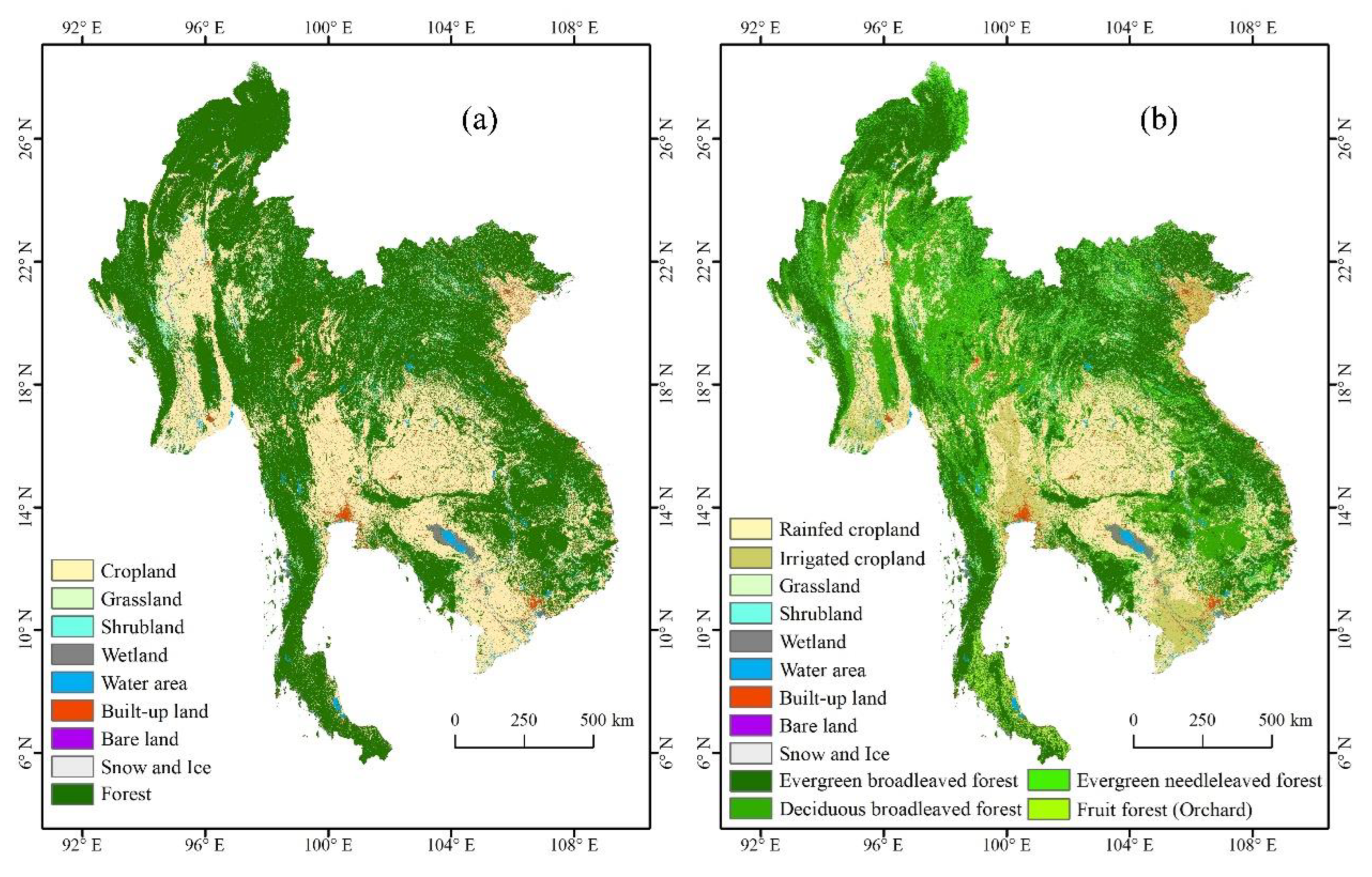
Based on the Bayesian-fuzzy probability prediction method, this study obtained 30 m resolution land use/cover fusion datasets in the Indochina Peninsula region in 2020 (BeyFusLUC30), as shown in Figure 3.

4.2. Consistency Analysis

Consistency checks can put all the pixels of the LUC dataset into the analysis, revealing how consistent they are overall quantitatively. We divided the 5 datasets into two groups and calculated the overall consistency (OC) of each combination. The results are shown in Figure 4, where darker colors indicate higher overall consistency. The BeyFusLUC30 combination had the highest OC content. Among them, the BeyFusLUC30/Globeland30 combination had the highest OC, 83.34%; the BeyFusLUC30/GLC_FCS30 combination had the lowest OC, 73.76%, but it was also 7–14% higher than the combination of GLC_FCS30 and other datasets.

Further, we arithmetically average the overall consistency of the 4 combinations in which each dataset is located to obtain the average overall consistency (AOC). Comparing the AOC between BeyFusLUC30 and the 4 source datasets, they are ranked from high to low: BeyFusLUC30 (79.57%) > Globeland30 (73.15%) > LSV10 (73.12%) > ESRI10 (69.39%) > GLC_FCS30 (65.96%). The AOC of BeyFusLUC30 was 6–14% higher than the source datasets.

4.3. Overall Accuracy Test

Accuracy validation was performed on five datasets, and the results are listed in

Table 3. Accuracy test results for 5 datasets.

Dataset	Land Type	User Accuracy (%)	Producer Accuracy (%)	Overall Accuracy (%)	Kappa Coefficient (%)
LSV10	Cropland	86.63	84.23	79.27	78.07
	Forest	91.26	85.07
	Grassland	90.36	46.26
	Shrubland	36.25	96.75
	Wetland	23.89	70.34
	Water area	90.75	90.03
	Built-up land	81.41	94.48
	Bare land	47.10	57.96
GLC_FCS30	Cropland	92.96	68.46	77.00	75.45
	Forest	93.49	85.05
	Grassland	42.39	49.26
	Shrubland	41.62	55.60
	Wetland	19.67	86.60
	Water area	88.79	92.88
	Built-up land	79.02	91.42
	Bare land	11.78	80.26
ESRI10	Cropland	82.30	86.74	78.92	77.69
	Forest	97.84	87.76
	Grassland	26.78	65.12
	Shrubland	44.13	40.71
	Wetland	31.62	94.41
	Water area	98.39	70.92
	Built-up land	70.34	94.65
	Bare land	56.76	61.64
Globeland30	Cropland	90.14	73.39	77.19	75.83
	Forest	90.67	82.28
	Grassland	65.36	48.63
	Shrubland	29.23	97.37
	Wetland	26.23	41.79
	Water area	81.23	88.34
	Built-up land	77.76	94.92
	Bare land	63.32	66.26
BeyFusLUC30	Cropland	84.89	85.65	84.11	83.05
	Forest	93.01	92.84
	Grassland	70.25	62.96
	Shrubland	56.00	57.53
	Wetland	50.98	52.00
	Water area	91.03	94.29
	Built-up land	86.00	93.48
	Bare land	67.39	70.45

. Analysis at the dataset level shows that in the study area, the overall accuracy (OA) of the source datasets was between 77.00% and 79.27%. The OA of BeyFusLUC30 was 84.11%, 4.84–7.11% higher than the source datasets. The Kappa coefficient of the source datasets was 75.45–78.07%; the Kappa coefficient of BeyFusLUC30 was 83.05%, which was 4.98–7.60% higher than that of the source datasets.

According to formulas 10 and 11, the difference between user and producer accuracy can reflect the quantitative relationship between the LUC sample and the land in the validated dataset. If the user accuracy is higher, the number it identifies is higher than the number of the land type in the sample. Analysis of land type accuracy in five datasets: for cropland, GLC_FCS30 had the highest user accuracy (92.96%) but the lowest producer accuracy (68.46%), so it contains more cropland than the sample. This also applies to Globeland30 and LSV10. ESRI10, on the other hand, is the opposite. In BeyFusLUC30, the user accuracy and producer accuracy of cropland were balanced at 84.89% and 85.65%, respectively, with a difference of only 0.76%.

For forest, the user accuracies of the source datasets were excellent, ranging from 90.67–97.84, but the producer accuracies were relatively poor, ranging from 82.28–87.76%. In BeyFusLUC30, the forest had the most balanced user and producer accuracy, 93.01% and 92.84%, respectively, with a difference of only 0.17%.

LSV10, GLC_FCS30, and BeyFusLUC30 showed higher accuracy for the water bodies, whereas Globeland30 and ESRI10 had relatively lower accuracy. The five datasets for built-up land showed that the user accuracy was lower than the producer accuracy. Among them, the difference between the two accuracies in LSV10 and BeyFusLUC30 was small, around 8%. The difference between the two accuracies in GLC_FCS30, ESRI10, and Globeland30 was large, exceeding 12% or even more than 24% in all cases.

For wetlands, the source datasets demonstrate that the user accuracy is much lower than the producer accuracy; the two accuracies in BeyFusLUC30 are more balanced. For grassland, shrubland, and bare land, the advantages of BeyFusLUC30 are more obvious. Its user and producer accuracies are often the highest among the five datasets, and the balance is also better.

Furthermore, since the source LUC datasets are made based on remote sensing images of 2020 or nearby years, we remove cloud effects from all landsat8 surface reflectance images (LANDSAT/LC08/C01/T1_SR) of 2020 based on Google Earth Engine and make an average image (Landsat ASR). We visually compared the five datasets with the standard false-color image of the Landsat ASR and selected the main land types (cropland, forest, grassland, shrubland, wetland, water bodies, and built-up land) for a detailed investigation; the results are shown in Figure 5. In terms of cropland, the area of cropland in GLC_FCS30 was significantly larger than that shown in Landsat ASR; the areas of cropland in LSV10, GLC_FCS30, ESRI10, Globeland30, and BeyFusLUC30 were similar, and the distribution and texture of cropland and built-up land in BeyFusLUC30 had the best matching degree with Landsat ASR.

For forests, the results of LSV10, GLC_FCS30, ESRI10, and BeyFusLUC30 were similar, which can better reflect the interlaced characteristics of the forest and other land types. Globeland30 had the worst accuracy, and many other land types were classified as forests. For grassland and shrubland, the consistency of different datasets varied greatly, and LSV10 and BeyFusLUC30 had the best consistency with Landsat ASR. For wetlands, ESRI10 and BeyFusLUC30 could distinguish the boundaries between the water bodies and wetlands and had better accuracy. For the water bodies, LSV10, GLC_FCS30, ESRI10, and BeyFusLUC30 all showed boundaries between large areas of water and other land types. Among them, GLC_FCS30 and BeyFusLUC30 had the best extraction results for small water areas. Globeland30 showed obvious misclassification, and large land areas were classified as water. For built-up land, except Globeland30, the other four datasets reflected the shape features and texture details of built-up land well.

Based on the above analysis results, it can be concluded that, compared with the source datasets, BeyFusLUC30 has the highest overall accuracy and Kappa coefficient. For different land types, BeyFusLUC30’s user accuracy, producer accuracy, and the balance of the two accuracies, as well as the comparison results with remote sensing images, have all improved.

4.4. F1-Score Test

Based on the above accuracy test results, we further compared and analyzed the F1 scores of various land types in the five datasets; the results are shown in Figure 6. In general, the F1 scores of the five datasets were higher for cropland, forest, water bodies, and built-up land. The F1 scores for grassland, shrubland, wetland, and bare land were lower, and all types of land in BeyFusLUC30 had the highest F1 scores of their kind.

Detailed analysis: BeyFusLUC30 exhibited less improvement in the F1 score for cropland, forest, water bodies, and built-up land. The F1 scores of these land types in BeyFusLUC30 increased by at least 0.40–2.29% and, at most, by 6.66–9.88% compared to the source datasets. On the one hand, these land cover types have obvious spectral and texture characteristics and good spatial continuity, so remote sensing classification can achieve high accuracy (their original F1 scores generally exceed 80%). From this point of view, they don’t have much room for improvement. On the other hand, because their areas were large, the correction had little effect on the overall results. Therefore, it is normal and easy to understand that their F1 scores improved less in the fusion results [43,44]. The F1 scores of BeyFusLUC30 for grassland, shrubland, wetland, and bare land were greatly improved. Compared with the source datasets, the F1 scores of these land types in BeyFusLUC30 increased by at least 4.02–5.82% and, at most, by 14.41–48.35%. The reason is that these land types are ambiguous in definition, their texture and spectral features are similar, and their classification accuracy is low; but, because this fusion method utilizes all prior knowledge, it can effectively improve the F1 score. However, because their areas were small, the correction had a large impact on the overall results.

Based on the above results, it can be concluded that BeyFusLUC30 improved the F1 score of each land type. A fusion method based on Bayesian fuzzy probability prediction can effectively improve the precision and recall of each land type.

5. Discussion

In this study, a LUC data fusion method based on Bayesian-fuzzy probability prediction was developed, and four high-resolution LUC datasets (LSV10, GLC_FCS30, ESRI10, Globaland30) and the Indochina Peninsula fusion LUC dataset (BeyFusLUC30) were developed. According to the test results, the reliability and accuracy of Bey-FusLUC30 were significantly better than those of the four source datasets, with an average overall consistency of 79.57%, an overall accuracy of 84.11%, and a Kappa coefficient of 83.05%. BeyFusLUC30 has a good consistency with the source datasets than the combination of the source datasets (approximately 10%). The balance between the two accuracies of the dataset (user accuracy and producer accuracy) has increased, so the accuracy of BeyFusLUC30 has been improved in terms of both land types and datasets. The F1 score of BeyFusLUC30 increased by 0.40–2.29% for cropland, forest, water bodies, and built-up land, and increased by 4.02–5.82% for grassland, shrubland, wetland, and bare land when compared to the optimal results in the source datasets. These metrics reflect the feasibility and reliability of the fusion methods.

On the other hand, we compared the accuracy of fusion results with the existing methods, as shown in

Table 4. Overall accuracy (OA) compared with other studies.

Reference Paper	Principle	Number of Input Datasets	Region	OA of Result (%)	Increase in OA (%)
Chen et al. [21]	Expert scoring	6	Yangtze River delta	87.08	1.65
See et al. [25]	Geographically weighted regression	3	Global	87.90	4.50
Fritz et al. [26]	Convergence of evidence	5	Global	82.40	1.22
Lu et al. [27]	hierarchical optimization synergy	5	China	78.65	2.38
This paper	Bayesian probability	4	Indochina Peninsula	84.11	4.84

. Although the overall accuracy of the fusion results obtained in different studies varies greatly, the overall accuracy improvement in this study is the most obvious when compared to the highest overall accuracy in the input data set. This also shows the reliability of the fusion method proposed in this paper.

This study points out that the overall accuracy of the five LUC datasets in the Indochina Peninsula is ranked from high to low as BeyFusLUC30 (84.11%) > LSV10 (79.27%) > ESRI10 (78.92%) > Globeland30 (77.19%) > GLC_FCS30 (77.00%). Among them, the four source datasets have a deviation of ±7% from the accuracy claimed by the original authors (the overall accuracy of LSV10, ESRI10, Globeland30, and GLC_FCS30 was 74.4%, 85.96%, 85.72%, and 81.4%, respectively) [12,13,14,15,16]. Considering that the accuracy assessment of the original authors was conducted on a global scale, this study was conducted in a specific region of the Indochina Peninsula. Therefore, the difference between these two is understandable. This also shows that the selection of validation samples had a major impact on the results. Given the difference between the accuracy of information claimed by global LUC datasets and the actual situation in the region, we suggest that scholars introduce regional samples to test their accuracy before carrying out research in a specific region [45]. More importantly, if these accuracy indicators are needed as input in the research, then regional accuracy verification is essential.

Using the fusion method, this study introduces a spatial relationship into the Bayesian formula, thereby increasing its practicality in the field of geosciences. Considering the difference in the quality of LUC sample datasets and the uncertainty of the validation process, this study used the results published by the original authors based on global-scale validation to determine prior probability and comprehensive posterior probability. These statistics are reliable, but they differ from reality in the Indochina Peninsula. Therefore, constructing regionalized, high-quality LUC samples or selecting authoritative LUC sample datasets for regional accuracy validation will be an important way to improve the accuracy of fusion results [46]. However, the accuracy of the source datasets largely determines the quality of fusion results [47]. Owing to the high accuracy of cropland, forest, water bodies, and built-up land in the source datasets and after the improvement of the fusion process, the user accuracy and producer accuracy in the results were extremely high. The F1 score was generally higher than 85% or even 93%. Although the accuracies and F1 score for grassland, shrubland, wetland, and bare land have improved significantly, they are still generally lower than 70%. On the one hand, introducing hyperspectral and/or multispectral aerial images with higher resolution can more accurately identify the difference between spectral and texture features to improve the classification accuracy of the source datasets. This will be an important basis for improving the accuracy of fusion products. On the other hand, in future research, it will be important to improve their accuracy by introducing image texture, structural features, ecological indicators (normalized difference vegetation index, leaf area index, phenological characteristics), and time-series change information for the fusion process to supplement the shortcomings of source datasets, which will also be of great significance in the field of land use/cover mapping.

6. Conclusions

In this study, we developed a LUC dataset fusion method based on Bayesian-fuzzy probability prediction. We applied it to Indochina Peninsula as a study area, based on four high-resolution LUC datasets (LSV10, GLC_FCS30, ESRI10, and Globeland30, with a spatial resolution of 10 m–30 m) to conduct fusion research. The highest-accuracy LUC dataset (BeyFusLUC30) is currently available for researchers and government agencies in the region.

The method evaluates the spatial relationship and uses accuracy validation information as prior knowledge, which is a maximum probability discriminant model. It is capable of correcting low-reliability pixel attributes and maintaining high-reliability pixel attributes. The fusion results had better average overall consistency (79.57%), overall accuracy (84.11%), and Kappa coefficient (83.05%) than the original dataset. The research also shows that the fusion results show a small improvement in the accuracy of the land types with good original accuracy (cropland, forest, water bodies, and built-up land) but a large improvement in the land types with poor original accuracy (grassland, shrubland, wetland, and bare land). We also propose possible ways to further reduce the uncertainty of the fusion process and improve the quality of the results, including considering a regional LUC accuracy test and providing more refined reference information.